Glacial heterogeneity in Southern Ocean carbon storage abated by fast South Indian deglacial carbon release

HAL Id: hal-03109190

https://hal.archives-ouvertes.fr/hal-03109190

Submitted on 21 Jan 2021

HAL is a multi-disciplinary open access

archive for the deposit and dissemination of

sci-entific research documents, whether they are

pub-lished or not. The documents may come from

teaching and research institutions in France or

abroad, or from public or private research centers.

L’archive ouverte pluridisciplinaire HAL, est

destinée au dépôt et à la diffusion de documents

scientifiques de niveau recherche, publiés ou non,

émanant des établissements d’enseignement et de

recherche français ou étrangers, des laboratoires

publics ou privés.

Distributed under a Creative Commons Attribution - NonCommercial| 4.0 International

License

abated by fast South Indian deglacial carbon release

Julia Gottschalk, Élisabeth Michel, Lena M. Thöle, Anja S. Studer, Adam P.

Hasenfratz, Nicole Schmid, Martin Butzin, Alain Mazaud, Alfredo

Martínez-García, Sönke Szidat, et al.

To cite this version:

Julia Gottschalk, Élisabeth Michel, Lena M. Thöle, Anja S. Studer, Adam P. Hasenfratz, et al.. Glacial

heterogeneity in Southern Ocean carbon storage abated by fast South Indian deglacial carbon release.

Nature Communications, Nature Publishing Group, 2020, 11 (1), �10.1038/s41467-020-20034-1�.

�hal-03109190�

Glacial heterogeneity in Southern Ocean carbon

storage abated by fast South Indian deglacial

carbon release

Julia Gottschalk

1,2

✉

, Elisabeth Michel

3

, Lena M. Thöle

1,4

, Anja S. Studer

5,6

, Adam P. Hasenfratz

1,7

,

Nicole Schmid

1

, Martin Butzin

8

, Alain Mazaud

3

, Alfredo Martínez-García

5

, Sönke Szidat

9

&

Samuel L. Jaccard

1,10

Past changes in ocean

14

_{C disequilibria have been suggested to re}

_{flect the Southern Ocean}

control on global exogenic carbon cycling. Yet, the volumetric extent of the glacial carbon

pool and the deglacial mechanisms contributing to release remineralized carbon, particularly

from regions with enhanced mixing today, remain insuf

ficiently constrained. Here, we

reconstruct the deglacial ventilation history of the South Indian upwelling hotspot near

Kerguelen Island, using high-resolution

14

_{C-dating of smaller-than-conventional foraminiferal}

samples and multi-proxy deep-ocean oxygen estimates. We

find marked regional differences

in Southern Ocean overturning with distinct South Indian

fingerprints on (early de-)glacial

atmospheric CO

2

change. The dissipation of this heterogeneity commenced 14.6 kyr ago,

signaling the onset of modern-like, strong South Indian Ocean upwelling, likely promoted by

rejuvenated Atlantic overturning. Our

findings highlight the South Indian Ocean’s capacity to

influence atmospheric CO

2

levels and amplify the impacts of inter-hemispheric climate

variability on global carbon cycling within centuries and millennia.

https://doi.org/10.1038/s41467-020-20034-1

OPEN

1_{Institute of Geological Sciences and Oeschger Center for Climate Change Research, University of Bern, Bern, Switzerland.}2_{Lamont-Doherty Earth} Observatory, Columbia University of the City of New York, Palisades, NY, USA.3Laboratoire des Sciences du Climat et de l’Environnement, LSCE/IPSL, CNRS-CEA-UVSQ, Université de Paris-Saclay, Gif-sur-Yvette, France.4Department of Earth Sciences, Marine Palynology and Paleoceanography, Utrecht University, Utrecht, Netherlands.5Max Planck Institute for Chemistry, Climate Geochemistry Department, Mainz, Germany.6Department of Environmental Sciences, University of Basel, Basel, Switzerland.7_{Geological Institute, Department of Earth Sciences, ETH Zurich, Zurich, Switzerland.}8 Alfred-Wegener-Institut Helmholtz-Zentrum für Polar-und Meeresforschung, Bremerhaven, Germany.9_{Department of Chemistry and Biochemistry and Oeschger Centre for} Climate Change Research, University of Bern, Bern, Switzerland.10_{Present address: Institute of Earth Sciences, University of Lausanne, Lausanne, Switzerland.}

✉email:jgottsch@ldeo.columbia.edu

123456789

P

ast changes in the

14

_{C inventory of the atmosphere cannot}

solely be attributed to variations in cosmogenic production

(Fig.

1

). The fraction of atmospheric

14

_{C changes}

unac-counted for by production changes (referred here to as

production-corrected

Δ

14

C

atm

) is believed to reflect large-scale reorganizations

of the atmospheric and oceanic respired (i.e.

atmosphere-unequi-librated) as well as preformed (i.e. atmosphere-equiatmosphere-unequi-librated)

carbon inventories with direct implications for atmospheric CO

2

(CO

2,atm

) levels

1,2

. As

14

C is a transient tracer (mean Libby life time

Τ = 8033 yr), ocean-versus-atmosphere

14

_{C disequilibria reflect}

the rate and efficiency of ocean-atmosphere carbon exchange, and

the strength of global-ocean overturning rates

3

_{, and by inference the}

accumulation of respired carbon in the ocean interior

4

_{. Ocean}

14

_C

disequilibria are often expressed as ventilation ages that are

esti-mated for instance based on co-existing fossil planktic

(surface-dwelling) and benthic (bottom-(surface-dwelling) foraminifera, which are

believed to faithfully capture the

14

_{C activity of the water mass they}

grew in. However, despite a number of

14

C ventilation age

recon-structions, important aspects of the past global carbon cycle remain

yet unresolved, such as the location and extent of the glacial

carbon-rich (

14

C-depleted) reservoir that may explain glacial CO

2,atm

minima

4,5

_{, the likely carbon transfer pathways during the last}

deglaciation

5–9

, and the rates of oceanic carbon release (uptake) and

associated CO

2,atm

increase (decrease)

4,10

.

Intervals of deglacial CO

2,atm

rise coincide with cold spells in

the northern-hemisphere, i.e. Heinrich stadial (HS) 1 and the

Younger Dryas (YD), as well as a concomitant rise in Antarctic

air temperature (the thermal bipolar seesaw; Fig.

1

). Both phases

are interrupted by stagnating CO

2,atm

levels, and warm climate

conditions in the North Atlantic, i.e. the Bølling Allerød (BA)

interstadial, yet cooling conditions in the Southern Ocean, i.e. the

Antarctic Cold Reversal (ACR; Fig.

1

). The main control of rising

deglacial CO

2,atm

levels (and concomitant decreasing

14

C

atm

levels) on millennial timescales is thought to be the upwelling of

deep CO

2

-rich water masses to the Southern Ocean surface

2,5,7,9

.

Southern Ocean upwelling is a highly localized process today that

is favored by the interference of the Antarctic Circumpolar

Current (ACC) with local bathymetry in regions often referred to

as upwelling hotspots

11,12

_(Fig.

₂

_{). One of these important regions}

is located in the South Indian Ocean, where the ACC impinges on

the Kerguelen Plateau (Fig.

2

, Supplementary Fig. 1), causing

elevated vertical mixing rates, enhanced cross-frontal exchange

and efficient export of subsurface waters to the north

11,12

_{. Despite}

the significant leverage of the Kerguelen Island area and similar

regions on carbon partitioning between the deep ocean and the

atmosphere today (Fig.

2

), little is known about their ventilation

history and impact on deglacial CO

2,atm

variations.

Constraints on the past evolution of these upwelling regions

can be gained by proxy-based ocean ventilation and oxygenation

reconstructions. However, limited carbonate preservation, low

abundances of foraminifera and/or uncertainties related to

tem-poral changes in surface-ocean reservoir ages

13

_{can pose}

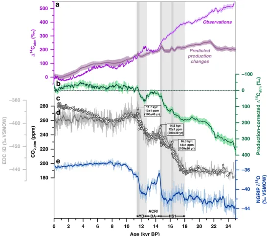
0 2 4 6 8 10 12 14 16 18 20 22 24 Age (kyr BP) –440 –420 –400 –380 EDC δD (‰ VSMO W) 180 200 220 240 260 280 CO 2,atm (ppm) 0 100 200 300 400 500 400 300 200 100 0 –100 Production-corrected Δ 14 Catm (‰) Δ 14 Catm (% o ) –44 –40 –36 NGRIP δ 18 O (‰ VSMOW) Observations Predicted production changes

a

b

c

d

11.7 kyr: 13±1 ppm (100±40 yr)

e

14.8 kyr: 12±1 ppm (200±30 yr) 16.3 kyr: 12±1 ppm (100±20 yr) ACR/ BA YD HS1

Fig. 1 Deglacial changes in atmospheric carbon dioxide levels. a Atmospheric radiocarbon (14_{C) concentrations referenced to modern (i.e. 1950) levels} (Δ14_{Catm, ShCal13, error bars show 1σ-standard deviations (SD))}26_{compared to predicted (i.e. modelled)}14_{C changes in the atmosphere due to variations} in cosmogenic production3_{(with error bars showing 1σ-SD), b production-corrected}3_{variations inΔ}14_C

atm, with error bars showing 1σ-SD, c atmospheric

CO2(CO2,atm) variations32, andd Antarctic temperature variations represented by water isotope changes,δD, in the Antarctic EPICA Dome C (EDC) ice

core25_{, ande water isotope changes,δ}18_{O, in Greenland ice core NGRIP}74_{. Vertical bars indicate intervals of rising CO}

2,atmlevels. Darker bars highlight

intervals of rapidly rising CO2,atmconcentrations at ~11.7, ~14.8, and ~16.3 kyr before present (BP)32. HS1 Heinrich Stadial 1, ACR Antarctic Cold Reversal, BA

significant challenges to reconstructing deglacial marine carbon

cycling in these regions. In addition, sedimentation in these areas

can be highly dynamic with common occurrences of

high-accumulation drift deposits

14,15

_{, often preventing robust age}

models to be developed. In particular, stratigraphic alignments of

sedimentary iron concentrations to Antarctic ice-core dust as

recently employed for the Southwest Indian Ocean

16

_{may be}

problematic as the lithogenic fraction may likely not be solely of

aeolian origin

17,18

. Many of these limitations were circumvented

through paired uranium series- and

14

_{C-dated corals in the Drake}

Passage upwelling hotspot region

8

_{complemented by deep-ocean}

14

_{C ventilation reconstructions from the South Atlantic}

5

_{. The}

data show a strengthening of upwelling and deep convection in

this region from the last ice age until 14.6 kyr before present (BP),

which likely contributed to the observed CO

2,atm

rise during HS1.

However, given the challenges and potential shortcomings

men-tioned above

16

_{, robust estimates of the deglacial evolution of}

ventilation changes in the deep (South) Indian Ocean are yet

limited. While intermediate-ocean

14

C-based ventilation

recon-structions offshore the Arabian Peninsula hypothesize two

dis-tinct upwelling events in the Indian sector of the Southern

Ocean

19

, this hypothesis remains untested and ultimately

trans-lates into highly uncertain past global carbon budgets associated

with the necessity of extrapolations to the deep Indian Ocean

4,10

_.

Here, we circumvent foraminiferal sample size requirements

for most conventional accelerator mass spectrometer (AMS)

systems (>1 mg CaCO

3

), and reconstruct the deglacial deep-ocean

ventilation history of the South Indian Ocean upwelling hotspot

east of the Kerguelen Plateau (Fig.

2

) via 138

14

C analyses of

small-sized, paired benthic (B) and planktic (P) foraminiferal samples

(0.2–1 mg CaCO

3

) from sediment core MD12-3396CQ (47°43.88′

S; 86°41.71′ E; 3,615 m water depth; Fig.

2

) with the

MIni-CArbon-DAting-System (MICADAS) at the University of Bern

20

_{, combined}

with multi-proxy bottom water oxygen estimates. We show based

on multiple lines of evidence that, while the deep South Indian

Ocean was a significant (remineralized) carbon sink during the last

glacial, marked glacial interbasin differences in carbon storage

existed in particular between the Atlantic and Indian sectors of the

Southern Ocean, likely due to more weakly ventilated, yet

geo-chemically distinct varieties of Antarctic Bottom Water (AABW).

The dissipation of these regional differences was mediated by a

reinvigoration of Southern Ocean mixing during the

first half of

HS1 and enhanced Atlantic overturning at the onset of the

BA interstadial, respectively, which we argue promoted a rise in

CO

2,atm

levels. We

find that increased Atlantic overturning at the

start of the BA period caused a homogenization of the entire South

Indian water column, both laterally and vertically, and hence is

considered to mark the onset of a modern-like upwelling hotspot

near Kerguelen Plateau. Our new

findings portray the South Indian

Ocean as a more active and distinct player in the global carbon

cycle and interhemispheric climate variability during the last

deglaciation than previously acknowledged.

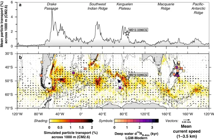
120°W 80°W 40°W 0° 40°E 80°E 120°E 160°E 160°W 120°W

70°S 60°S 50°S 40°S 30°S 0 0.5 1 1.5 2 0 1 2 3 MD12-3396CQ Southwest Indian Ridge Kerguelen Plateau Macquarie Ridge Pacific-Antarctic Ridge Drake Passage

Simulated particle transport (%) across 1000 m (CM2.6) 0 2 4 6 MD12-3396CQ Shading: Symbols:

Deep water d14R_B-Atm (kyr) LGM-Modern

Mean particle transport (%)

across 1000 m (CM2.6) Vectors: 0.05 m/s

Mean

current speed

(1–3.5 km)

a

b

Fig. 2 Regions of intense interaction of the Antarctic Circumpolar Current with local bathymetry in Southern Ocean upwelling hotspots. a Zonal variations in the percentage of upwelling particles transport crossing the 1000-m water depth surface (averaged between 30–70°S) as obtained in simulations with the Geophysical Fluid Dynamics Laboratory’s Climate Model version 2.6 (CM2.6)11_{, where particles were released between 1–3.5 km} water depth along 30°S. Increased particle transport in the simulations highlightsfive major topographic upwelling hotspots in the Southern Ocean11_. b Spatial changes in particle transport in percent across the 1000 m-depth surface, with vectors showing the average speed and direction of ocean currents at mid-depth (1–3.5 km) based on the Global Ocean Data Assimilation System (GODAS) database (https://psl.noaa.gov/data/gridded/data.godas.html) representing the Antarctic Circumpolar Current between 40–60°S. Squares indicate reconstructed deep-water14_{C ages in the Southern Ocean during the} last glacial maximum (LGM) referenced to preindustrial10,16_{. Star in both panels shows the location of the study core. Figure modified after ref.}11_.

Results

Deglacial variations in upper ocean temperatures. Our study

takes advantage of a comprehensive age model approach based on

a stratigraphic alignment of multi-proxy (sub-)sea surface

tem-perature ((sub-)SST) records and Antarctic air temtem-perature as

recorded in Antarctic ice cores. We reconstructed (sub-)SST

variations at our study site based on three independent

for-aminiferal and lipid biomarker proxies (i.e. forfor-aminiferal

assem-blages

21

_{, planktic foraminiferal Mg/Ca ratios}

22

_{, and the TEX}

L

86

-paleothermometer

23

_{; Methods). All temperature proxy records}

closely resemble Antarctic temperature variability (Fig.

3

), and

reconstructed late Holocene values agree well within uncertainties

with the present-day annual SST range at the core site (7.2–8.4 °C,

0–50 m average)

24

_(Fig.

₃

_{). We assess (sub-)SST variability}

independently of the uncertainties inherent to each proxy based

on the

first principal component (PC1) of all three datasets

(Fig.

3

), which accounts for 77% of the data variance. Under the

assumption of thermal equilibrium between sub-Antarctic and

Antarctic temperatures

5

, we graphically align PC1 with Antarctic

air temperature recorded by

δD variations in the Antarctic

EPICA Dome C (EDC) ice core

25

_(Fig.

₃

_{, Supplementary Figs. 2–}

4). The obtained tiepoints provide estimates of local

surface-ocean reservoir age (d

14

_R

P-Atm

) variations (Fig.

4

, Supplementary

Fig. 5). Using these d

14

_R

P-Atm

constraints, we correct and

cali-brate our 95 planktic foraminiferal

14

_{C dates based on the}

atmospheric ShCal13 calibration

26

, and calculate a sediment

deposition (i.e. a chronological) model for our study core

(Methods, Supplementary Fig. 6).

Surface-ocean reservoir age changes. High-resolution

14

C dates

(Methods

20

_{) obtained from small monospecific planktic}

for-aminiferal samples (Neogloboquadrina pachyderma) in gaseous

(0.24–1.07 mg CaCO

3

; n

= 57) and graphite form (0.63–1.15 mg

CaCO

3

; n

= 7) show a steady down-core

14

C age increase without

age reversals that exceed 2σ-uncertainties (Fig.

3

; Supplementary

Fig. 5). Gas

14

C analyses of small samples are consistent within

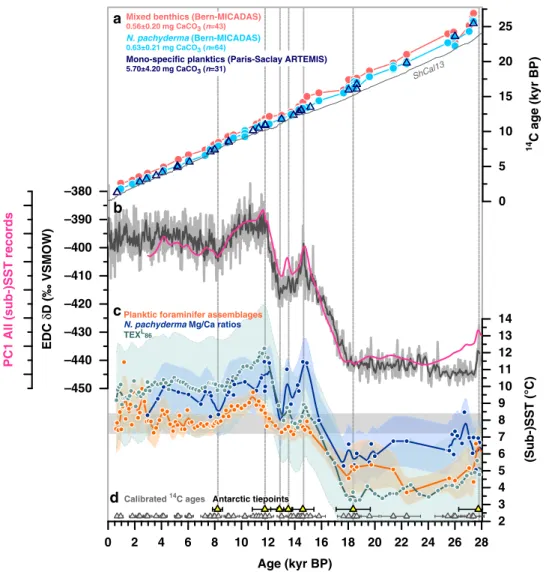
0 2 4 6 8 10 12 14 16 18 20 22 24 26 28 Age (kyr BP) –450 –440 –430 –420 –410 –400 –390 –380 EDC δ D (‰ VSMOW) 2 4 5 6 7 8 9 10 11 12 13 14 (Sub-)SST (°C)

PC1 All (sub-)SST records

0 5 10 15 20 25 14 C age (kyr BP)

b

a

c

d

Calibrated 14C ages Antarctic tiepoints

Mixed benthics (Bern-MICADAS) 0.56±0.20 mg CaCO3 (n=43) N. pachyderma (Bern-MICADAS) 0.63±0.21 mg CaCO3 (n=64)

Mono-specific planktics (Paris-Saclay ARTEMIS) 5.70±4.20 mg CaCO3 (n=31)

Planktic foraminifer assemblages

N. pachyderma Mg/Ca ratios

TEXL 86

ShCal13

3

Fig. 3 Chronostratigraphy and foraminiferal radiocarbon dates in sediment core MD12-3396CQ. a Benthic foraminiferal (red) and Neogloboquadrina pachyderma14_{C dates (light blue) obtained with the Bern-Mini Carbon Dating System (MICADAS, gas and graphite}14_{C analyses), as well as planktic} foraminiferal14_{C dates obtained with conventional accelerator mass spectrometry (AMS) dating at the ARTEMIS laboratory at the University of} Paris-Saclay (open symbols; graphite analyses), grey line shows atmospheric14_{C ages (ShCal13)}26_{, see Supplementary Fig. 5 for more details,bfirst principal} component (PC1) of our three (sub-)sea surface temperature (SST) records (pink) and Antarctica air-temperature variations represented by the EPICA Dome C (EDC)δD record25_{(grey),c planktic foraminiferal assemblage-based}21_{summer SST changes (orange), TEX}L

86-based23sub-SST estimates

(green), and N. pachyderma Mg/Ca-based22_{SST variations (blue), envelopes indicate the 1σ standard deviation-uncertainty range (smoothed), and} d tiepoints between (sub-)SST variations recorded in MD12-3396CQ and_{δD variations in the EDC ice core}25,69_{(yellow and vertical stippled lines, see also} Supplementary Figs. 2 and 3), and calibrated planktic foraminiferal14_{C dates (grey). Horizontal bar inc indicates the modern SST range at the core site} (7.2–8.4 °C, 0–50 m average; World Ocean Atlas 2013)24_.

100 ± 70

14

_{C yr (n}

_{= 7) with those made on larger graphitized}

samples (0.59–13.75 mg CaCO

3

; n

= 31), despite a sample mass

difference up to a factor of ~8 (Fig.

3

; Supplementary Fig. 5)

20

_.

We estimate d

14

_R

P-Atm

variations through subtracting

atmo-spheric

14

C ages, derived from our 10 calendar (cal.) tiepoints,

from our interpolated (high-resolution) planktic

14

_{C age}

record (Fig.

4

, Supplementary Fig. 5). We

find that reconstructed

d

14

R

P-Atm

ages deviate from preindustrial (i.e. prebomb)

surface-ocean reservoir ages of 700 ± 150 yr at our study site (Fig.

4

,

Supplementary Fig. 5)

27,28

_{. Specifically, d}

14

_R

P-Atm

values during

the last glacial and the early/late deglacial warming intervals were

elevated by up to 800 and 200 yr, respectively (Fig.

4

). In contrast,

the Holocene and the brief deglacial period of the ACR

show lower d

14

R

P-Atm

values by up to 400 yr (Fig.

4

). Our

proxy data-based constraints on d

14

_R

P-Atm

are supported by

transient simulations of marine reservoir ages in the study area

(80–100°E, 45–50°S; Fig.

4

a) that are forced by temporal changes

in

Δ

14

_C

atm

(Methods

29

). Specifically, our glacial reconstructions

resemble modelled d

14

_R

P-Atm

under glacial boundary conditions,

while d

14

R

P-Atm

values broadly agree with simulations under

present-day climate boundary conditions beyond the ACR

(Fig.

4

a). Although uncertainties in our d

14

_R

P-Atm

estimates

including chronological, analytical and calibration errors

(Meth-ods) are nontrivial, changes in surface-ocean reservoir ages at our

study site match with proxy-data-based d

14

_R

P-Atm

reconstruc-tions from the Southwest Pacific

30,31

_{, the Chilean margin}

7

_and,

apart from one mid-glacial datapoint, the South Atlantic

5

(Fig.

4

a). In contrast, our reconstructions disagree with the

deglacial d

14

R

P-Atm

variability recently inferred for the Kerguelen

Plateau region

16

_{on millennial timescales (Fig.}

₄

_a).

0 2 4 6 8 10 12 14 16 18 20 22 24 26 Age (kyr BP) 400 300 200 100 0 –100 Production-corrected Δ 14 C atm (‰) –440 –420 –400 –380 EDC δ D (% o VSMOW) 2.0 1.5 1.0 0.5 0.0 2.0 1.5 1.0 0.5 0.0 2.5 2.0 1.5 1.0 0.5 d 14 R B-Atm ( 14 C kyr) d 14 RP-Atm ( 14 C kyr) d 14 R B-P ( 14 C kyr) 180 200 220 240 260 280 CO 2,atm (ppm)

a

b

c

d

Glacial simulation Interglacial simulation

e

ACR/ BA YD HS1 Interglacial simulation Glacial simulation

Fig. 4 Deglacial ocean reservoir age variations reconstructed in South Indian core MD12-3396CQ. a Surface-ocean reservoir age (d14_{RP-Atm) constraints} from the Southern Ocean for the deglacial and glacial periods: Chilean Margin (MD07-3088, light green, tephra-based)7_{, in the New Zealand area} (orange30_{, red}31_{, tephra-based), in the sub-Antarctic Atlantic (MD07-3076CQ, dark green, stratigraphic alignment between sea surface temperature} (SST) and Antarctic temperature)5_{, and in the South Indian (MD12-3396CQ, light blue, stratigraphic alignment between (sub-)SST and Antarctic} temperature). d14_R

P-Atmvalues for the Kerguelen Plateau adopted by ref.16are shown in dark red (for locations of cores see inset map),b

benthic-to-planktic foraminiferal14_{C age offsets (d}14_R

B-P) in MD12-3396CQ,c14C age offsets of benthic foraminifera in MD12-3396CQ from the contemporaneous

atmosphere, d14_R

B-Atm,dΔ14Catmvariations corrected for changes in cosmogenic14C production3, ande atmospheric CO2(CO2,atm) changes (black

symbols)32_{and EPICA Dome C (EDC)δD variations (grey)}25,69_{. Grey lines ina and c show simulated d}14_{RP-Atmchanges at the study site (80–100°E,} 45–50°S; Methods29_{) at 25 m and 3.5 km depth, respectively. Arrow inc indicates prebomb deep-ocean reservoir ages (1.3}14_{C kyr) at our study site} (according to the the Global Ocean Data Analysis Project database, version 2)28_{. Lines and envelopes show 1 kyr-running averages and the 1σ-uncertainty/} 66%-probability range. Vertical bars indicate intervals of rising CO2,atmlevels (darker bands highlight periods with centennial-scale CO2,atmincreases32).

Deglacial deep-ocean 14C disequilibria in the South Indian

Ocean. Our study site is bathed by Lower Circumpolar Deep Water

(LCDW), underlain by AABW and overlain by Indian Deep Water

(IDW, Methods and Supplementary Fig. 1), and is thus ideally

located to document the temporal evolution of vertical mixing due

to its sensitivity to changes in northern- (emanating from the North

Atlantic) and southern-sourced water masses (originating primarily

from Adélie Coast and the Ross Sea). This can be achieved by

determining past changes in deep-ocean

14

_{C disequilibria that are}

reflected in

14

_{C age offsets between deep water (benthic}

for-aminifera) and the surface ocean (planktic forfor-aminifera) (d

14

R

B-P

)

as well as the contemporaneous atmosphere (d

14

_R

B-Atm

).

We observe slightly higher d

14

_R

B-P

values at our core site

during the last glacial maximum (LGM, i.e. from 23–18 kyr BP)

(900 ± 250 yr, n

= 6) when compared to the Holocene (last 11 kyr

BP: 600 ± 200 yr, n

= 14; Fig.

4

b). Rapid decreases in d

14

_R

B-P

values occur at the end of the early- and late deglacial (Fig.

4

b).

Consistent with our d

14

R

B-P

record, reconstructed d

14

R

B-Atm

values are significantly elevated during the LGM (2300 ± 200 yr,

n

= 6) compared to the Holocene (1100 ± 200 yr, n = 14) (Fig.

4

c).

They further show an abrupt d

14

R

B-Atm

decrease at the onset of

the early deglacial warming and rising CO

2,atm

levels at ~18.3 kyr

BP, but an increase to glacial-like conditions shortly thereafter

(Fig.

4

c). Although this feature is constrained by only one paired

14

_{C measurement, it is independently supported by bottom water}

oxygen reconstructions, as discussed below. The strongest

deglacial change in d

14

R

B-Atm

occurs at ~14.6 kyr BP, when

d

14

_R

B-Atm

rapidly decreases by 1500 ± 300

14

C yr within 600 ±

400 cal. yr in parallel with a CO

2,atm

increase

32

of 12 ± 1 ppm at

the onset of the ACR and BA (Figs.

4

c,

5

). The deep South Indian

Ocean remained well-ventilated during the ACR, when d

14

_R

B-Atm

ages are lower by up to 500 yr than prebomb values (Fig.

4

c). Late

deglacial (i.e. YD) warming in the southern high latitudes

coincides with a rise of d

14

_R

B-Atm

ages. At ~11.7 kyr BP, however,

d

14

_R

B-Atm

rapidly drops by 450 ± 250

14

C yr within 850 ± 400 cal.

yr, paralleling a marked centennial-scale CO

2,atm

rise

32

of 13 ± 1

ppm (Fig.

5

). Reconstructed mean late Holocene d

14

R

B-Atm

values

at our core site (1200 ± 200 yr) agree well with prebomb values

(Fig.

4

c)

28

_{. Numerical simulations forced by changes in air-sea}

CO

2

exchange through transient changes in

Δ

14

C

atm

and CO

2,atm

(Methods

29

_{) also broadly agree with our reconstructed}

deep-ocean ventilation ages during the late deglaciation and Holocene,

while they significantly underestimate deep-ocean reservoir ages

during the LGM and early deglaciation (Fig.

4

c).

Our deep South Indian ventilation ages closely resemble those

found further downstream at mid-depth of the Southwest

Pacific

30,33

_{(1.6–3 km; Fig.}

₅

_{). In contrast, upstream in the South}

Atlantic at 3.8 km water depth

5

_{(a site chosen because of a}

comparable hydrography and methodological approach used for

our study core), glacial d

14

R

B-Atm

values are found to be much

larger by 300–1500

14

_{C yr than at our study site (Fig.}

₅

_{), which is}

also reflected in differences in epibenthic δ

13

_{C and}

_δ

18

_{O records}

34

(Supplementary Fig. 9). However, d

14

R

B-Atm

values in both regions

converge and decrease simultaneously (within age uncertainties) at

~14.6 kyr BP and with identical magnitude (~1500

14

_{C yr) (Fig.}

₅

_e,

f), and share similar variability thereafter. During the subsequent

ACR, reduced ventilation ages in both the deep South Indian and

South Atlantic Oceans closely agree with intermediate water

estimates from south of Tasmania (1.4–1.9 km)

35

_{and with the}

mid-depth Southwest Pacific Ocean (1.6–2.3 km; Fig.

5

e, f)

30,33

_{. A}

similar convergence can be observed at the end of the late deglacial

warming interval, i.e. the end of the YD (Fig.

5

c, d).

Deglacial bottom water oxygenation changes. The diagenetic

precipitation of insoluble (authigenic) U compounds in marine

sediments and in foraminiferal coatings is redox-driven, with

oxygen-depleted conditions in pore waters favoring the

enrich-ment of aU (Methods). At our South Indian study site, changes in

bulk sedimentary aU levels during the last deglaciation closely

parallel reconstructed variations in d

14

R

B-Atm

ages (Fig.

6

), and

are entirely consistent with changes in the enrichment of U

compared to Mn in authigenic coatings of foraminifera (Fig.

6

).

A more quantitative bottom water [O

2

] indicator at our study site

is provided by the

δ

13

_{C difference between the benthic foraminifera}

Globobulimina sp. and Cibicides sp., the

Δδ

13

_{C proxy}

36

_{. This proxy}

is thought to reflect the oxygen-driven respiration of organic matter

in marine subsurface sediments, and is thus a direct measure of

bottom water [O

2

] (Methods

36

). Applying the most recent

Δδ

13

C-[O

2

] calibration

36

, we

find that bottom water [O

2

] during the LGM

was lowered by 100 ± 40 µmol kg

−1

from present-day

concentra-tions (~220 µmol kg

−1

; Fig.

6

)

37

_{, which is consistent with higher}

d

14

_R

B-Atm

values, increased sedimentary aU enrichments and higher

foraminiferal U/Mn ratios (Fig.

6

). In contrast to our d

14

R

B-Atm

- and

bulk sedimentary aU records, we do not observe a marked

Δδ

13

C-based bottom water [O

2

] change during the early deglaciation,

suggesting that any bottom water [O

2

] change during this interval

must have been confined to within the proxy uncertainty, i.e.

80 µmol kg

−1

, if it existed at all. Our foraminiferal

Δδ

13

_C

data additionally highlight a rapid bottom water [O

2

] increase

of 50 ± 40 µmol kg

−1

at the end of the early deglacial warming at

14.6 kyr BP in parallel with the rapid reductions in d

14

_R

B-Atm

, aU

levels and foraminiferal U/Mn ratios (Fig.

6

).

Discussion

Enhanced deep South Indian Ocean carbon storage during the

LGM. An isolated glacial deep-ocean

14

_{C-depleted carbon}

reser-voir that accommodated more respired carbon during the LGM

has been proposed to explain the last glacial CO

2,atm

minimum

4

.

Marine

14

_{C proxy evidence supports the existence of such a}

reservoir in the Pacific Ocean

30,38

_{, in the deep South Atlantic}

5

and in the deep North Atlantic

39

. Larger-than-Holocene

d

14

_R

B-Atm

(and d

14

R

P-Atm

) values (Fig.

4

), lower

Δδ

13

C-derived

glacial bottom water [O

2

] and enhanced glacial aU accumulation

at our study site (Fig.

6

) extend those observations to the Indian

sector of the Southern Ocean, which is consistent with recent

findings from the Crozet and Kerguelen Plateau regions

16

_.

Assuming negligible saturation- and/or disequilibrium [O

2

]

changes, our multi-proxy reconstruction highlights a substantially

higher accumulation of respired carbon throughout the deep

Indian Ocean basin during the LGM than during the

Holocene. The last glacial ventilation age increase at our South

Indian core site is about twice that of the global LGM ocean

mean

4,10

_(Fig.

₄

_{), similar to observed trends in the Atlantic}

5

_and

Pacific

33

_{sectors of the Southern Ocean (Fig.}

₅

_{). We thus argue}

that large swaths of the Southern Ocean accommodated an

above-average share of the global-ocean respired carbon at the

LGM, largely contributing to the observed glacial reduction in

CO

2,atm

through decreased upwelling and ocean-atmosphere CO

2

exchange.

The observed ventilation age and

Δδ

13

_{C-derived oxygen}

changes of glacial South Indian deep waters at our study site

are unlike any preindustrial water mass of the deep Atlantic and

Indian Oceans, but instead resemble the oldest prebomb

deep-water masses of the Pacific Ocean (Fig.

7

). As North Atlantic

Deep Water (NADW)

flow to the glacial Indian Ocean was

diminished

40

_{, the glacial (South) Indian increase in respired}

carbon storage may be related to reduced formation and/or

overturning rate of southern-sourced water masses (i.e. AABW)

and/or reduced air-sea CO

2

equilibration in the Southern Ocean

during the LGM. Adjustments of AABW were likely closely

linked to a reduction in shelf space around Antarctica owing to

advancements of Antarctic ice sheet grounding lines

41

, an

expansion of Antarctic sea ice cover

42

_{, and an associated shift}

of the mode and locus of AABW formation, from super-cooling

underneath shelf ice and brine rejection in polynyas

43

to

open-ocean convection off the shelf break during the last glacial

44,45

_.

However, open-ocean convection during the LGM may have been

localized and seasonal in nature (possibly facilitated by

open-ocean polynyas) in all sectors of the Southern Ocean, and

therefore less efficient at ventilating the ocean interior. Physical

and biological changes in the South Indian Ocean are crucial in

explaining the last glacial increase in respired carbon content,

because simulated adjustments in air-sea gas exchange alone

cannot explain our proxy data (Fig.

4

). Therefore, a possible

northward shift of the southern-hemisphere westerly wind belt

46

and northward expansion of Antarctic sea ice may have changed

the geometry of Southern Ocean density surfaces

47

_{, in particular}

relative to the location of the Kerguelen Plateau, which combined

with more poorly ventilated AABW may have curtailed the

capacity of the Kerguelen Plateau region to act as a hotspot for

the upwelling of CO

2

-rich water masses to the surface and

subsequent air-sea equilibration.

180 200 220 240 260 280 CO 2,atm (ppm) 4.0 3.5 3.0 2.5 2.0 1.5 1.0 0.5 d 14 RB-Atm ( 14C kyr) d 14 RB-Atm ( 14 C kyr) 2 4 6 8 10 12 14 16 18 20 22 24 26 Age (kyr BP)

a

14 14.5 15 15.5 16 Age (kyr BP) 225 230 235 240 245 CO 2,atm (ppm) 3.0 2.5 2.0 1.5 1.0 0.5 d 14 RB-Atm ( 14C kyr) 11 11.5 12 12.5 Age (kyr BP) 245 250 255 260 265 270 275 CO 2,atm (ppm) 2.5 2.0 1.5 1.0 0.5

b

This study (MD12-3396CQ, 3.6 km WD) Hines et al., 2015 (Tasmanian corals, 1.4-2 km WD) Skinner et al., 2010 (MD07-3076CQ, 3.8 km WD) Skinner et al., 2015 (MD97-2121, 2.3 km WD) Sikes et al., 2016 (New Zealand, 1.6-3.5 km WD)

c

d

e

f

ACR/ BA YD HS1

Fig. 5 Deglacial deep-ocean reservoir age variations in the Southern Ocean. a, c, e Benthic foraminiferal14_{C age offsets in MD12-3396CQ (3.6 km water} depth, WD) from the contemporaneous atmosphere, d14_R

B-Atm(blue), compared to deep-ocean ventilation ages in the deep sub-Antarctic Atlantic

(MD07-3076CQ, 3.8 km WD; upstream, green5_{), on the Chatham Rise (MD97-2121, 2.3 km WD; downstream, orange}30_{), in the New Zealand area} (1.6-3.5 km WD; downstream, red33_{), and south of Tasmania (corals, 1.4–1.9 km WD; downstream, purple}35_{), andb, d, f atmospheric CO}

2(CO2,atm) changes.

Lower panels zoom in on d14_R

B-Atmvariations during specific intervals of rapid centennial CO2,atmincrease32, i.e. the ~11.7 (c, d) and ~14.8 kyr events (e, f).

Lines and envelopes show 1 kyr- (a) and 0.5 kyr- (c–f) running averages and 1σ-uncertainty-/66%-probability ranges. Vertical bars indicate intervals of rising CO2,atmlevels (dark bands highlight periods with centennial-scale CO2,atmincreases)32. HS1 Heinrich Stadial 1, ACR Antarctic Cold Reversal, BA

Glacial-ocean heterogeneities in Southern Ocean carbon

sto-rage. Comparison of our new data with existing

paleoceano-graphic

reconstructions

suggests

common

water

mass

characteristics in the Indian and Pacific sectors of the Southern

Ocean during the LGM, yet significant offsets exist with the deep

central South Atlantic (Fig.

5

). We can rule out that this observed

LGM offset is a methodological artifact. First, a consideration of

foraminiferal blanks in the reconstruction of d

14

_R

B-Atm

at our

study site, although critically discussed

20

_{, can only explain a small}

fraction of the observed glacial difference (Supplementary Fig. 7).

Second, glacial d

14

_R

P-Atm

estimates in South Atlantic core

MD07-3076CQ reach values larger than 2000 years during the LGM

5

_,

which may be unrealistic according to a new compilation

48

.

Disregarding these extreme d

14

_R

P-Atm

values (following similar

sensitivity tests made by ref.

8

_{) reduces but does not eradicate the}

observed LGM d

14

R

B-Atm

mismatch with our South Indian study

site (Supplementary Fig. 8). Further supported by glacial offsets in

benthic foraminiferal stable isotopes

34

_{(Supplementary Fig. 9), we}

consider the observed interbasin heterogeneity in both d

14

_R

B-Atm

and

Δδ

13

_{C-derived [O}

2

] values (Fig.

7

) to be realistic, and argue

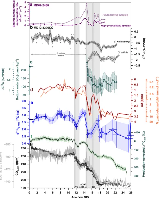
0 2 4 6 8 10 12 14 16 18 20 22 24 26 Age (kyr BP) –440 –420 –400 –380 EDC δD (‰ VSMOW) 3.0 2.5 2.0 1.5 1.0 0.5 0.0 d 14 RB-Atm ( 14 C kyr) 180 200 220 240 260 280 CO 2,atm (ppm) 10 1 0.1 20 2 5 0.2 0.5 N. pachyderma

U/Mn (mmol mol

–1 ) 4 3.5 3 2.5 2 1.5 1 0.5 0 aU (ppm) –2.5 –2 –1.5 –1 –0.5 0 0.5 δ 13 C (‰ VPDB) 50 100 150 200 Bottom water [O 2 ] (µmol kg –1) 400 300 200 100 0 –100 Production-corrected Δ 14 Catm (‰) 0 1 2 3 4 5

Benthic foraminiferal accumulation rate

(# cm –2 yr –1 ) G. affinis

b

MD12-3396CQ

c

d

e

f

h

g

1 1.5 2 Δδ 13 C (‰ VPDB) C. kullenbergi G. affinis absent

a

MD02-2488 Phytodetritus species High-productivity species ACR/ BA YD HS1

Fig. 6 Deglacial oxygenation and deep-ocean reservoir age variations in the South Indian Ocean. a Accumulation rates of benthic foraminifera indicative of phytodetrital input (light purple) and high annual productivity (dark purple) in core55_{MD02-2488,b benthic foraminiferalδ}13_{C records from} MD12-3396CQ (black (epibenthic/shallow infaunal species): Cibicides kullenbergi, grey (deep infaunal species): Globobulimina affinis; small symbols: replicate analyses, large symbols: mean values),cδ13_{C gradient between G. affinis and C. kullenbergi (Δδ}13_{C), and corresponding}36_{bottom water [O}

2] levels at our

study site (arrow indicates present-day bottom water [O2]37; small circles show theΔδ13C range based on non-averaged G. affinis δ13C values), diamonds

show average values,d authigenic U (aU) levels (brown) and U/Mn ratios in authigenic coatings of N. pachyderma (orange) in MD12-3396CQ, e d14_R

B-Atm

variations (arrow shows prebomb values, following the Global Ocean Data Analysis Project database, version 2)28_{measured in core MD12-3396CQ,} f production-corrected3_{variations inΔ}14_{Catm,g atmospheric CO2(CO2,atm) variations (circles)}32_{, andh EPICA Dome C (EDC)δD changes (grey line)}25,69_. Vertical bars indicate intervals of rising CO2,atmlevels. Darker bands highlight periods with centennial-scale CO2,atmincreases32. Lines and envelopes inb, c

ande show 0.5 kyr-running averages and the 1σ-uncertainty/66%-probability range, respectively. HS1 Heinrich Stadial 1, ACR Antarctic Cold Reversal, BA Bølling Allerød, YD Younger Dryas.

that they may be explained by distinct sources, modes of

for-mation and/or end-member characteristics of southern-sourced

water masses in the glacial Southern Ocean. Present-day

differ-ences in the location of AABW formation across the three sectors

of the Southern Ocean

43,49

might have been amplified during the

LGM owing to reduced NADW inflow

40

_{and concomitant}

expansion of AABW

5

_{. These deep-ocean processes are likely}

insufficiently captured in the simulations of glacial deep-ocean

reservoir ages of ref.

29

_{, in particular because of their dependence}

on subgrid processes (Fig.

4

). As strong regional differences in the

surface

14

_{C equilibration timescale}

50

_{, the surface-ocean O}

2

solu-bility

51

, and respiration rates in the glacial Southern Ocean are

unlikely, we conclude that the observed South Atlantic–South

Indian offsets in LGM bottom water characteristics may instead

be explained by differences in AABW formation and in the

degree of ocean-atmosphere CO

2

equilibration

44

.

The glacial ocean stored an estimated surplus of ~700–1000

GtC, which may explain ~70–100% of the observed

glacial-to-interglacial CO

2,atm

change

4,10,52

, although there remains

sub-stantial uncertainty

53

_{regarding the magnitude of terrestrial}

biosphere loss during the last ice age. However, these estimates

required extrapolations to the Indian Ocean basin, as direct

observations were lacking. Converting the observed

Δδ

13

C-derived LGM-Holocene [O

2

] offset of 100 ± 40 µmol kg

−1

at

our South Indian study site into respired carbon change following

existing protocols

6,52

_{, we}

_{find an increase in remineralized carbon}

level of 55–115 µmol kg

−1

_(Fig.

₆

_{, Methods). This is lower or at}

the lower end of estimates from the South Atlantic (116–144

µmol kg

−1

)

6

_{and the equatorial Pacific (98–119 µmol kg}

−1

₎

52

_,

which corroborates our earlier assertion of spatial nuances in the

glacial-ocean respired carbon increase across ocean basins. These

nuances need to be considered in order to robustly quantify the

ocean contribution to glacial CO

2,atm

minima.

Transient early deglacial ventilation increase in the South

Indian Ocean. At the onset of HS1, deep-ocean

14

C ventilation

(Fig.

5

) and oxygenation in the South Indian (as indicated by the

aU record in MD12-3396CQ, Fig.

6

) and in the South Atlantic

5

increased until 16.3 kyr BP, signaling a net loss of (remineralized)

carbon from the deep ocean during that time interval. A

com-parison to simulated deep-ocean reservoir changes in our study

region implies that atmospheric

14

C variability transmitted into

the deep ocean cannot explain the observations (Fig.

4

). Instead,

this early deglacial ocean-carbon release was likely driven through

an early deglacial reduction in Antarctic sea ice cover (promoting

air-sea gas exchange)

5

, increased vertical mixing through AABW

reinvigoration

54

_{and -formation below ice shelves and within}

coastal/shelf polynyas (as shelf space becomes available), and/or a

poleward shift/reinvigoration of the southern-hemisphere

wes-terlies and associated Ekman pumping of subsurface waters

9

_.

These combined or in isolation might have altered the water

column density structure near Kerguelen Plateau in such way that

isopycnals increasingly interfered with the local bathymetry,

leading to reinvigorated vertical mixing

11,12,47

_{during the}

_{first half}

of HS1.

We hypothesize that increased South Indian vertical mixing

during early HS1 would have fueled biological productivity

through the supply of nutrient-rich water masses to the euphotic

zone of our study region

17

. This is documented in nearby core

MD02-2488 (46°28.8′S, 88°01.3′E; 3420 m water depth) by

enhanced accumulation of benthic foraminiferal species

indica-tive of highly seasonal and high surface-ocean productivity as

these benthics feed on labile organic matter raining out of the

euphotic zone (Fig.

6

)

55

_{. A transient supply of labile phytodetrital}

organic carbon to the sediment may also help explain the

insensitivity of the

Δδ

13

_C-[O

2

] proxy as a result of ecological

biases

56

_{of C. kullenbergi and/or G. affinis during that time}

4 3.5 3 2.5 2 1.5 1 0.5 0

Conventional 14C age (kyr) Conventional 14C age (kyr) Conventional 14C age (kyr)

4 3.5 3 2.5 2 1.5 1 0.5 0 0 50 100 150 200 250 300 [O 2 ] ( μ mol kg –1 ) 4 3.5 3 2.5 2 1.5 1 0.5 0 80°S 40°S 0 40°N 80°N

Latitude Ocean basin Atlantic Indian Pacific

13 14 15 16 17 18 19 20 22 14 15 17 18 19 21 22 14 15 17 18 19 21 22 Pacific Ocean >2 km

a

Atlantic Ocean >2 km

b

Indian Ocean >2 km

c

GLODAPv2 MD07-3076CQ GLODAPv2 MD12-3396CQ (this study) GLODAPv2 9 10 11 12 13 15 16 17 18 9 10 11 12 13 15 16 17 18 TR163-23

Fig. 7 Relationship between seawater oxygen concentrations and conventional radiocarbon ages at present-day and in the past. Modern seawater [O2]

levels versus conventional14_{C age ina the Atlantic Ocean (squares), b Indian Ocean (circles), and c Pacific Ocean (triangles) below 2 km water depth}28_; modified after ref.4_{. Symbol color represents the latitude of the seawater sample. Large symbols show reconstructed bottom water [O}

2] (via theΔδ13C

proxy) and ventilation ages (i.e. d14_{RB-Atm, representing paleo-conventional}14_{C ages) from the deep South Atlantic (green: MD07-3076CQ, 3.8-km water} depth)5,6_{, the deep South Indian (blue, this study: MD12-3396CQ, 3.6-km water depth) and the deep Eastern Equatorial Pacific Ocean (black: sediment} core TR163-23, 2.7 km water depth72,73_{; please note that HoloceneΔδ}13_{C proxy data in this core overestimate present-day bottom water [O}

2] in the study

region by ~80µmol kg−1). Symbol labels indicate temporal bins over which the paleo-14_C-[O

2] data were averaged (in kyr before present (BP), e.g. for

15 kyr BP: 15.99_{–15 kyr BP). The principal trend of increasing ventilation ages with decreasing seawater oxygen content can be ascribed to the accumulation} of respired carbon, while deviations from this trend can be driven by the advection of well-ventilated water masses, e.g. from the Weddell Sea ([O2]

increase without14_{C change), or through organic carbon respiration in upwelling regions ([O}

2] decrease without14C change)4. On multi-millennial

timescales, the respiration rate may change (causing the14_C-[O

2] slope to steepen orflatten), and the ocean-atmosphere14C and O2equilibration

timescales change with varying atmospheric CO2levels (i.e. mean reservoir ages increase in a glacial 190 ppm-CO2atmosphere without [O2] change)50

(Fig.

6

). Nonetheless, the observed increase in ventilation (via

biology-independent paleo-indicators), marine productivity (via

benthic foraminiferal response) and in bottom water oxygenation

(via aU) during early HS1 provide strong evidence for enhanced

upwelling of CO

2

-rich water masses and/or strengthened upper

ocean-atmosphere CO

2

equilibration in the South Indian Ocean,

which contributed to the early deglacial rise in CO

2,atm

levels

~18.3 to ~16.3 kyr ago.

A unique feature of the deep South Indian Ocean amongst

other existing (

14

_{C and O}

2

) ventilation age records from south of

40°S relates to a ventilation decrease, and thus a return to

glacial-like conditions during late HS1, starting at ~16.3 kyr BP (Fig.

6

).

Our data signal a restratification of the South Indian water

column during late HS1, which may be controlled by changes in

the ventilation and formation of South Indian deep waters, for

instance by increases in AABW salinity, along with a shift of the

southern-hemisphere westerlies to south of the Kerguelen

Plateau

57

. A reduction in carbon release from the South Indian

to the atmosphere during late HS1, likely due to an unfavorable

superposition of the South Indian water column density structure

with bathymetry around Kerguelen Island, may have halted

the early deglacial CO

2,atm

rise and promoted the plateauing of

CO

2,atm

between ~16.3 and ~14.8 kyr BP (Fig.

4

)

32

. The fact that

this late HS1 return to glacial-like conditions in

14

C and O

2

ventilation is not observed in the South Atlantic

5,6

_{or elsewhere in}

the Southern Ocean indicates that interbasin differences persisted

throughout HS1, attributing the South Indian Ocean a unique

role in modulating deglacial CO

2,atm

variability.

Flushing of the Southern Ocean carbon pool through AMOC

reinvigoration. The marked glacial and early deglacial

geo-chemical interbasin heterogeneity abruptly dissipated at the end

of HS1, when the ventilation age and oxygen characteristics of

deep waters in the different ocean basins rapidly approached

prebomb values for the

first time throughout the deglaciation

(Fig.

7

). We argue that the fast increase in

14

C and O

2

ventilation

in the South Indian Ocean at the end of HS1, at ~14.6 kyr BP, is

linked to a rapid resumption of Atlantic overturning at the onset

of the BA warm period

58

, causing a rapid (decadal to

centennial-scale) southward expansion

59

_{and eastward deflection of NADW}

towards the Indian Ocean via the ACC. This may have caused a

flushing of the deep-ocean carbon pool that is not only limited to

the equatorial Atlantic

60

but expanded into the South Atlantic

5,8

and South Indian Ocean (this study), with remarkable,

near-identical ventilation changes in the latter two regions and a much

wider spatial impact on the global ocean than previously

recog-nized (Fig.

5

a). These

flushing events were possibly amplified by a

lagged response of sea ice to a rapid shift of the

southern-hemisphere westerlies northward

57,61

, allowing an unabated,

transient evasion of carbon from the Southern Ocean to the

atmosphere and likely more efficient Ekman pumping around

Kerguelen Plateau. These changes might have also impacted the

geometry of Southern Ocean isopycnals relative to the location of

the Kerguelen Plateau or underlying bathymetry, causing elevated

mesoscale eddy activity, diapycnal exchange and/or upwelling

along isopycnal surfaces in our study area

11

_{. An associated}

transient upwelling event of CO

2

and nutrient-rich water masses

to the surface ocean at the BA onset is supported by a second

abrupt local abundance peak of benthic foraminiferal species that

reflects upwelling-driven phytoplankton blooms (Fig.

6

). Our

data hence suggest that a large fraction of the concomitant 12 ± 1

ppm CO

2,atm

increase was driven by a rapid loss of carbon from

the South Indian Ocean associated with the reinvigoration of

Atlantic overturning and wind-driven Ekman pumping. This

transient upwelling event also heralded the establishment of the

South Indian upwelling hotspot at ~14.6 kyr BP that was akin, if

not stronger than its present-day counterpart.

A new equilibrium in air-sea gas exchange, however, was

reached during the subsequent ACR period, when vertical mixing

in the southern, high latitudes was seemingly stronger than at

present-day as shown by lower-than-prebomb ventilation ages in

the deep South Atlantic

5

_{, in the South Indian (this study) and in}

the Southwest Pacific

33

_(Fig.

₅

_{a). Because our South Indian}

ventilation age reconstructions closely match similar data from

the deep South Atlantic

5

_{, the Southwest Pacific}

30,33

_and

intermediate water depths south of Tasmania

35

during the ACR

(Fig.

5

, Supplementary Fig. 9), we argue that reinvigorated

deep-ocean ventilation led to a remarkably homogeneous water column

in large parts of the Southern Ocean both laterally and vertically

during that time. Given an expansion of Antarctic sea ice cover

61

and northern-hemisphere warming reducing the ocean CO

2

solubility

62

_{during the ACR, the capacity of the South Indian}

Ocean to impact CO

2,atm

levels during that time was likely limited

despite high mixing rates, which is consistent with the observed

CO

2,atm

plateau during the ACR (Fig.

5

a, b).

Late deglacial South Indian ventilation decrease and early

Holocene convergence. During the YD, we observe decreased

14

_{C and O}

2

ventilation at our deep South Indian study site,

suggesting that the South Indian remained a moderate source of

carbon to the atmosphere, and thus did not significantly

con-tribute to the late deglacial CO

2,atm

increase. This agrees with

inferences made in other Southern Ocean regions

5,7,8

_{, but}

dis-agrees with recent

findings from the South Indian Ocean

16

_{. We}

show that the disagreement results from insufficiently accounted

surface-ocean reservoir age variability that can be improved by

applying consistent surface-ocean reservoir ages for all sites

(Supplementary Fig. 10). At the end of the YD, we observe a

convergence of ventilation ages of different parts of the Southern

Ocean, reminiscent of the 14.6 kyr BP-event (Fig.

5

,

Supple-mentary Fig. 9). We argue that this convergence may have caused

a large fraction of the 13 ± 1 ppm-CO

2,atm

increase at that time

through a rapid loss of carbon from the South Indian Ocean

mediated by stronger Atlantic overturning and wind-driven

Ekman pumping. This reinforces the role of the South Indian

Ocean in centennial-scale CO

2,atm

variability during the last

deglaciation.

Based on our high-resolution multi-proxy analyses, we identify

marked impacts of marine carbon cycling in the South Indian

Ocean on glacial and deglacial CO

2,atm

variations. While our new

high-resolution data support previous contentions of reduced

vertical mixing and restricted air-sea gas exchange in all sectors of

the Southern Ocean during the last ice age, they point to marked

spatial differences, possibly due to lateral variations in the mode

and rate of AABW formation and/or the efficiency of air-sea gas

equilibration. We argue that major increases in South Indian

convection during the early HS1 as well as the ends of the

YD-and HS1 stadials as shown by both

14

_{C (d}

14

_R

B-Atm

) and O

2

ventilation proxies (aU,

Δδ

13

_{C and foraminiferal U/Mn) affected}

deglacial CO

2,atm

variability significantly and rapidly. However,

these changes alone cannot explain reconstructed

14

_{C ventilation}

ages in the mid-depth North Indian Ocean off the Arabian

peninsula during deglacial northern-hemisphere stadials

19

_.

Glacial and early deglacial spatial differences in deep-ocean

ventilation and oxygenation were entirely eroded along with the

southward expansion of northern-sourced water masses at the

onset of the ACR, with potentially strong effects on CO

2,atm

levels

owing to the

flushing of old carbon from the deep ocean

including the Indian Ocean. We interpret this to mark the onset

of the upwelling dynamics akin to the present-day hotspot region