Predicted signatures of pulsed reconnection in ESR data

HAL Id: hal-00316245

https://hal.archives-ouvertes.fr/hal-00316245

Submitted on 1 Jan 1996

HAL is a multi-disciplinary open access

archive for the deposit and dissemination of sci-entific research documents, whether they are pub-lished or not. The documents may come from teaching and research institutions in France or abroad, or from public or private research centers.

L’archive ouverte pluridisciplinaire HAL, est destinée au dépôt et à la diffusion de documents scientifiques de niveau recherche, publiés ou non, émanant des établissements d’enseignement et de recherche français ou étrangers, des laboratoires publics ou privés.

Predicted signatures of pulsed reconnection in ESR data

C. J. Davis, M. Lockwood

To cite this version:

C. J. Davis, M. Lockwood. Predicted signatures of pulsed reconnection in ESR data. Annales Geo-physicae, European Geosciences Union, 1996, 14 (12), pp.1246-1256. �hal-00316245�

Ann. Geophysicae 14, 1246—1256 (1996) ( EGS — Springer-Verlag 1996

Predicted signatures of pulsed reconnection in ESR data

C. J. Davis, M. Lockwood

Space Science Department, Rutherford Appleton Laboratory, Chilton, Didcot, Oxfordshire OXII OQX, UK Received: 5 February 1996/Revised: 3 June 1996/Accepted: 10 June 1996

Abstract. Early in 1996, the latest of the European inco-herent-scatter (EISCAT) radars came into operation on the Svalbard islands. The EISCAT Svalbard Radar (ESR) has been built in order to study the ionosphere in the northern polar cap and in particular, the dayside cusp. Conditions in the upper atmosphere in the cusp region are complex, with magnetosheath plasma cascading freely into the atmosphere along open magnetic field lines as a result of magnetic reconnection at the dayside mag-netopause. A model has been developed to predict the effects of pulsed reconnection and the subsequent cusp precipitation in the ionosphere. Using this model we have successfully recreated some of the major features seen in photometer and satellite data within the cusp. In this paper, the work is extended to predict the signatures of pulsed reconnection in ESR data when the radar is pointed along the magnetic field. It is expected that en-hancements in both electron concentration and electron temperature will be observed. Whether these enhance-ments are continuous in time or occur as a series of separate events is shown to depend critically on where the open/closed field-line boundary is with respect to the radar. This is shown to be particularly true when recon-nection pulses are superposed on a steady background rate.

1 Introduction

The European incoherent-scatter (EISCAT) radars have been in operation in northern Scandinavia since 1983 (Rishbeth and Williams, 1985). This facility, with a tri-static UHF radar and effectively two monotri-static VHF radars, has proved extremely useful in furthering our understanding of the coupled upper atmosphere-iono-sphere-magnetosphere system at high latitudes. In 1996,

Correspondence to: C. J. Davis

the existing radars will be complemented by an additional facility on Svalbard. At 78.2°N, 15.82°E, the EISCAT Svalbard Radar (ESR) is in an ideal position to study the dynamics of the upper atmosphere in the polar cusp region and the dayside polar cap (Cowley et al., 1990). These regions are threaded by field lines which have been reconnected with the interplanetary magnetic field (IMF) relatively recently. Thus these regions are connected by magnetic field lines to the dayside magnetopause, across which some shocked solar-wind plasma of the mag-netosheath is transferred (Reiff et al., 1977; Lockwood, 1995a, b; Cowley, 1982). Mechanisms for this mass trans-fer which have been suggested include wave-driven dif-fusion and penetration by high-momentum solar-wind filaments. However, both observational and theoretical evidence strongly indicates that magnetic reconnection is the dominant process. Magnetopause observations and recent ground-based radar and optical observations, as well as low-altitude satellite data, all strongly suggest that the magnetopause reconnection rate is pulsed (see the review Lockwood, 1995a). In this paper, we offer some predictions as to what the ESR will see under conditions of pulsed reconnection.

The output from a time-dependent, self-consistent aur-oral precipitation model (Palmer, 1995) was used to model the spatial and temporal distribution of 630-nm atomic oxygen emission in response to pulsed magnetopause re-connection. In this way, it was possible to simulate how such events would appear to a meridian scanning photo-meter in the cusp region. By making assumptions about the nature of the reconnection, the model was shown to be able to match some of the major features seen in photo-meter and satellite observations. This work has been sub-mitted for publication and is currently under review.

In this paper we consider those output parameters of the auroral model which are observable to incoherent scatter (such as electron concentration, Ne, and ion and electron temperatures, ¹i and ¹e). In this way, it is pos-sible to extend the previous work to predict what would be seen by the ESR. In principle, it is possible to vary the

reconnection rate used as an input to the model between fully pulsed (i.e. there is no background reconnection taking place between the pulses) and the opposite limit of continuous and steady reconnection. For the illustrative purpose of this paper however, we will limit ourselves to two cases with square wave pulses in reconnection rate, namely fully pulsed reconnection and reconnection pulses during which the rate is twice the steady background value between the pulses.

2 The model

2.1 Estimating the reconnection pattern

Reconnection between the IMF and the geomagnetic field occurs on the dayside magnetopause. In order to study the effects of pulsed reconnection, it is necessary to estimate certain parameters defining the reconnection-rate vari-ation. We do this by referring to magnetopause observa-tions of the effects of reconnection. A study has been made of the temporal distribution of magnetopause flux transfer events (FTEs) (Lockwood and Wild, 1993), which are widely considered to be signatures of pulsed mag-netopause reconnection. The conclusions of this study were that reconnection occurred in bursts, lasting on average 2 min with a mean repeat period of 8 min. The most common (mode) values of the periods and pulse durations were 2 min and 35 s, respectively (Lockwood and Davis, 1995). In our model, we use a reconnection variation with a 4-min period, reconnection occurring in a square wave pulse lasting 1 min in each cycle. The repeat period, although lower than the mean repetition rate seen in satellite data, comes well within the observed distribu-tion, and was chosen as a compromise between the mean and the mode of the observations (Lockwood and Wild, 1993). Similarly, a duration of 1 min was chosen as a com-promise between the mean and the mode of the observed distribution.

On reconnection, the resultant open field line is bent, and contracts under the influence of the curvature (‘‘ten-sion’’) force and later because of the antisunward magneto-sheath flow. The point where the open field line threads the boundary typically moves at &150—400 km s~1 over the magnetopause. If the reconnection occurs in bursts, the pulses of enhanced tangential magentopause electric field asscoiated with these motions are not in general mapped down into the ionosphere as they would be in steady state (Lockwood and Cowley, 1992). The response time of ionospheric flows and electric fields is set by the frictional drag caused by ion-neutral collisions and the inductance of the dayside magnetosphere. Observations and theory suggest this time to be of the order to 20 min. Theoretical estimates of the inductive smoothing constant have been calculated by many authors (Holzer and Reid, 1975; Sanchez et al., 1991; Coroniti and Kennel, 1973; Lockwood and Cowley, 1992). Observational evidence comes from studies of the response of dayside flows (meas-ured using the EISCAT radar) to IMF changes (monitored with the AMPTE satellites), which showed that although flows responded within 5 min of a change

impinging on the dayside magnetopause, they sub-sequently continued to evolve over a further period of about 15 min (Todd et al., 1988, Etemadi et al., 1988). Thus the time to establish the full flow corresponding to the new IMF orientation is of the order of 20 min. For pulsed reconnection occurring at a rate that is faster than this, the changes in magnetospheric magnetic fields mean that the pulses of magnetopause electric field are induc-tively smoothed out in the ionosphere in the Earth’s frame of reference. During continual pulsed reconnection with a sufficiently short repetition period, to a good approxi-mation the ionosphere at the foot of newly reconnected field lines moves poleward at a constant velocity (Lock-wood et al., 1993b). In our model, we assume that pulsed reconnection has been occurring for some time before the observations start and that there is a constant 500-m s~1 poleward plasma velocity in the ionosphere. Consecutive bursts of reconnection will give contiguous patches of ionospheric plasma on open field lines, and these will convect polewards with the constant convection velocity (Cowley et al., 1991).

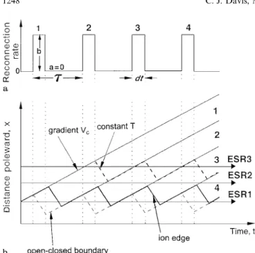
The location of the reconnection site is variable. It is dependent on the geometry of the magnetosheath field relative to the geomagnetic field, and is therefore sensitive to changes in the direction of the IMF. If a large compo-nent of the IMF exists along the direction of the Earth’s orbit (the By component), the reconnection site will be altered in longitude. In addition, the subsequent reconnec-ted field lines will evolve over the polar cap in an asym-metric pattern because the tension force has a component in the ½ direction the size of which is dependent on the exact geometry. In this paper, we shall assume a subsolar reconnection site and neglect these effects of the IMF By component. This allows us to limit the model to the two-dimensional case in which the field line evolves along the Sun-Earth meridian from a subsolar reconnection site. The top panel of Fig. 1 shows the model reconnection-rate variation used in this paper. In this figure, the background reconnection rate is a, and the enhanced reconnection rate is b. The repeat period used is q"240 s and the square wave pulses last dt"60 s. The reconnection rate is zero between the pulses in Fig. 1, so the mean value is one-quarter of the value within the pulses. Section 3 will consider a second case of pulsed but continuous reconnec-tion in which there is a steady background reconnecreconnec-tion rate between the pulses.

2.2 Mapping the precipitation into the ionosphere

The positions of the field lines in the ionosphere and their response to the reconnection is shown in the lower panel of Fig. 1. In this figure, the position of a field line along a magnetic meridian, shown by the distance x (defined as positive poleward), is plotted against time, t. During a burst of reconnection, the open/closed (o/c) field-line boundary (shown as a thin dashed line in this diagram) erodes equatorwards, only relaxing back when the recon-nection stops and the o/c boundary convects polewards with the same speed as the (constant) poleward plasma flow (Lockwood et al., 1993b). Note that the o/c boundary

Fig. 1. a Reconnection-rate variation showing square wave pulse, labelled 1—4, dt long and of repeat periodq. The rate within the pulses is b, that between the pulses, a, is here zero. b Distance of field lines, along the magnetic meridian, x, as a function t. The boundaries between patches 1—4 (opened by pulses 1—4) move polewards with the constant poleward convection speed, »c. Three lines of constant time elapsed since reconnection are shown: the thin dashed line is ¹"_{0 (i.e. the o/c boundary); the thick solid line is ¹+120 s (i.e. the} ion edge); and the thick dashed line is the ¹ at which precipitation flux decays to below the threshold which defines it as cusp (i.e. the poleward edge of the cusp). The mean latitude of the o/c boundary is taken to be constant. The horizontal lines marked ESR1, ESR2 and ESR3 show the locus of the radar for the locations, relative to the mean o/c boundary, which give rise to the variations shown in Fig. 6a, b and c, respectively

deliniates the two regions of closed and open field-line topography. It therefore responds instantly when field lines are reconnected (i.e. their topology is altered from closed to open). In the examples presented here, the mean drift of the boundary is taken to be zero when averaged over several cycles of the reconnection-rate variation. This is here adopted for simplicity and the effects of a boundary drift will be discussed later. Poleward of the o/c boundary is the open flux, where magnetosheath plasma is free to cascade into the ionsphere. Once reconnected, this mag-netosheath plasma crosses the magnetopause by flowing along the field line and is accelerated as the field line convects polewards (Cowley, 1982; Lockwood, 1995a). As the ions flow down the field line to the ionosphere, they undergo a velocity filter dispersion (Rosenbauer et al., 1975; Shelley et al., 1976; Reiff et al., 1977). For adiabatic, scatter-free motion of zero pitch angle ions, they move at all times at the velocity corresponding to the energy they acquire on crossing the magnetopause. Thus the most energetic ions arrive in the ionosphere first, followed by particles of decreasing energy. The flux of the electrons appears to be governed by that of the ions in order for the plasma to maintain quasi-neutrality (Burch, 1985). In the ionosphere, at the foot of the field line, there is a delay of around 2 min from the moment of reconnection to the

arrival of significant fluxes of the plasma, corresponding to the time of flight of the most energetic ions, after which the energy of the precipitating ions decreases and fluxes both of ions and electrons increase. The x at which the ions, and thus the larger fluxes of electrons first arrive is called the ‘ion-edge’ and is represented as the bold solid line in Fig. 1. Because the arrival time and flux of the ions and the position of the field line in the ionosphere are all functions of time elapsed since the field line was reconnec-ted, ¹, it is possible to model the intensity of the precipita-tion along the meridian as a funcprecipita-tion of time elapsed since reconnection. A construction like that shown in Fig. 1b is used to evaluate ¹ as a function of both x and t. The inclined thin lines in the lower panel of Fig. 1 show the field lines opened at the start of each reconnection pulse, they therefore delineate the patches of newly opened flux (1—4) produced by the corresponding reconnection pulses in the upper panel. These lines have a gradient »c, the poleward velocity of the plasma. This inductively smoothed velocity corresponds to the mean reconnection rate (here one-quarter of the peak value). The diagram also shows an example of a locus of the position of a constant time elapsed since reconnection, ¹ (as a thick dashed line). Because ¹ (x, t) is known, and because the ion precipitation flux is known as a function of ¹, we can compute the meridional profile of the flux at any instant of time.

2.3 The auroral model

The model described in the previous section can predict where the precipitation will occur, and what its flux will be, but in order to determine the effect that this precipita-tion would have on the ionosphere, we used an auroral model, which, for a given spectrum of precipitation, solves the chemical and transport equations in one dimension (Palmer, 1995). This model uses multistream electron transport code which has been described elsewhere (Lum-merzheim, 1987; Rees and Lum(Lum-merzheim, 1989). The in-itial neutral atmosphere was modelled using the MSIS 90 model (Hedin, 1991) which was run for moderate solar (F10.7"100) and geomagnetic (Ap"15) activity. The concentrations of a range of minor neutral and ion species were then calculated by time integrating the continuity equations on a one-dimensional, field-aligned grid (85 up to 500 km) using a comprehensive ion chemistry scheme based on previously published reactions (Rees, 1989). Ver-tical and horizontal transport of the ion and neutral species were neglected. In order to avoid confusing this with the model of field-line motion described in the pre-vious section, in this paper we will refer to it as ‘the auroral model’.

The cusp electron spectrum which was input into the auroral model was Maxwellian in shape, with a character-istic energy of 100 eV and a total energy flux of 5 mW m~2 (corresponding to a temperature of 1.16]106 K and a concentration of 4.7]10~7 m~3). Such a spectrum has been classified as typical of an ‘‘active’’ cusp (Carlson and Egeland, 1995) in which transient events are seen. Although in our model we assume that the electron

precipitation does not change within the cusp region, this is not always the case. There are many examples of satel-lite data which show spatial structure in the electron flux. We do not know exactly how this structure varies, but there is some evidence that bursts of enhanced electron flux are caused by the satellite encountering small struc-tures which move polewards at the convection velocity (Lockwood et al., 1993b). That being the case, we would expect Fig. 5 to contain more polewards-moving structure than is shown and more complex structure in Figs. 6a—c and 8. If each event is associated with the same electron-flux structure and variation, this added detail will be regular and periodic. Such a situation is implied by the periodic structure in photometer data (Sandholt et al., 1992). One possible explanation of such structure in the electron flux is the presence of field-aligned currents (FACs).

In the present state of development, the auroral model can only calculate the effect of electron precipitation, which limits the information that can be determined about the exact amount of ionisation, heating and excita-tion taking place, as the effect of the precipitating ions is unknown. In general, it is expected that the ion precipita-tion would increase the overall electron concentraprecipita-tion and heating. However, as the behaviour of the ions varies with time elapsed since reconnection, it is likely that the iono-spheric effects of such ions will evolve in the same way. There is no agreement or model as yet as to the iono-spheric effect of the cusp ion precipitation. The ions will raise the ionospheric electron temperature and concentra-tion and therefore the 630-nm optical emission, but to an unknown extent. It is hoped to include ion precipitation in our model at a later date. This inclusion of ion precipita-tion would alter the evoluprecipita-tion of Ne, ¹e and 630-nm emission rate within each event, but not the relation of events in time and space. The main purpose of this paper is to discuss the relation of events to each other and to satellite signatures, which can be achieved by looking at the electron precipitation alone.

When running the auroral model it was assumed that once a flux tube has been opened (¹"0) the sheath plasma will flow toward the ionosphere and precipitation effects would be seen as soon as sufficient flux reaches the ionosphere (at ¹+2 min, the time of flight of the most energetic ions); precipitation classified as ‘‘cusp’’ has been shown to last for about 10 min (Lockwood and Davis, 1995) (until ¹+12 min). Subsequently sheath plasma flows super-Alfve´nically into the tail and the precipitation is switched off. The auroral model was then run with constant cusp electron precipitation between ¹"2 and 12 min, and then run for a further 10 min to allow for the effects of the precipitation to decay. Although cusp elec-tron precipitation shows considerable structure, a square wave pulse of precipitation is typical of the gross features of observed electron spectra. The implications of such an approximation have been discussed above. It has been shown for a specific example (Newell et al., 1991, plate 1) that the reconnection rate was steady (to within a factor of two) (Lockwood et al., 1994). The range of lower cut off ion energies in the cusp region seen during this particular pass have also been used to estimate that cusp

precipita-tion lasted for 10 min on each field line (Lockwood and Davis, 1995). From this example, it can be seen that, although the ion spectrum ramps down in energy with time, the electron spectrum can be broadly represented by a square wave pulse. Therefore we can make the first-order assumption that the electron flux and energy spec-trum is constant within the cusp region. Thus we can use the approximate electron precipitation model with a single square wave pulse of flux which has an elapsed time since reconnection lasting 600 s. As the model out-lined in Sect. 2.2 describes the distribution of time elapsed since reconnection along the meridian at any one time, it thus becomes possible to reconstruct the latitudinal pro-file of the precipitation as a function of time and from this, calculate the features that would be seen by various in-struments.

The auroral model is one dimensional, which means it does not allow for any drift of the excited neutral oxygen atmosphere, relative to the field lines down which the sheath plasma precipitates. Thus a further simplifying assumption made by the model is that the poleward com-ponent of the thermospheric wind, »n, is the same as the poleward convection speed, »c. This is significant for the predictions of 630-nm emissions because the neutral oxy-gen atoms are excited to the1D2 state and decay back to the3P ground state with the emission of a 630-nm photon, only after a radiative lifetime which averages 110 s at great altitudes. The mean lifetime is somewhat less at lower heights, where the excited1D2 states tend to be quenched by collisions rather than de-exciting by emission of the photon. During the lifetime of the excited state, Dt, the neutral atom will in general move (»n!»c) Dt from the field line on which the precipitation occurred. By taking »n"»cwe thus neglect this effect which will, because of the range ofDt, tend to smear latitudinal structure in the 630-nm emission in real cases (where »n(»c). If we re-gardDt as varying with altitude between 20 and 110 s, for a »n of 500 m s~1, with a »c of 1 kms~1, this effect would smear a sharp precipitation boundary over a distance of 45 km.

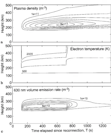
The auroral model predicts the electron concentration and temperature of the ionospheric plasma on a field line with a known history of cusp electron precipitation. It also gives the volume emission rate of 630-nm light, which is largely excited by the hot tail of the heated thermal ionospheric electrons. Panels of Fig. 2 show (from top to bottom) the variations of Ne and ¹e and the 630-nm volume emission rate as a function of ¹, for a pulse of cusp electron precipitation lasting 10 min, between, ¹"120 and 720 s.

2.4 Modelling satellite observations

Satellites overflying the cusp will measure the spectra of the precipitating ions and electrons. A variety of patterns in the ion precipitation can result if the reconnection is pulsed (Lockwood and Smith, 1994). The concepts intro-duced in this paper have been used to model the stepped cusp forms (Lockwood and Davis, 1995) that have been observed (Lockwood et al., 1993a; Pinnock et al., 1993).

Fig. 2a–c. Variations of parameters predicted by the auroral model as a function of ¹ and h, for a square wave variation of electron precipitation flux between ¹"120 s and ¹"720 s. a Ne, from 1]e11 to 8]e11 m~3; b ¹e from 500 to 2000 K and c the volume emission rate at 630 nm from 1]e10 to 6]e10 m~3

These predictions are discussed briefly here, as we wish to study the relationship of events seen by the ESR with the steps seen by the satellites.

As the satellite flies through the region, the ion spec-trum it will detect will vary according to the distribution of time elapsed since reconnection of the field lines it crosses (¹ ). The evolution of the ion spectrum that is seen therefore depends very strongly on the direction of the satellite pass. A low-altitude satellite (with a height &

800 km) moves at a speed, »s, of roughly 8 km s~1. We here consider two satellites; The first, S, moves meridi-onally equatorwards such that dx/dt"!»s; the second, S1, also moves equatorwards, but has a large longitudinal component to its motion such thatDdx/dtD@»s. The satel-lite S, crossing the cusp from pole to equator, (line S in Fig. 3) will initially see low-energy ions as it crosses the field lines opened during the first burst of reconnection (i.e. with a high ¹ ). Within each region, the energy of the ions will increase slightly, as the satellite moves towards the field lines opened later in the pulse: this occurs because the satellite moves equatorwards sufficiently quickly that it samples field lines of progressively lower ¹. At the boundary between regions 1 and 2 (opened by reconnec-tion pulses 1 and 2, respectively) the satellite moves across a discontinuity in ¹. Region 2 has lower values of ¹ than region 1, because pulse 2 occurred after pulse 1, and so the energy of the ion precipitation there is greater. The next boundary crossing will be similar, but the ion

precipita-Fig. 3. Same as precipita-Fig. 1b, but showing the loci of the meridionally equatorwards-moving, low-altitude satellite, S, and a longitudinally moving low-altitude satellite which also moves slowly equator-wards, S1

tion there will have a higher energy still. In this way, the overall shape of the observed ion spectrum will appear as ramps rising to higher energies, with discontinuous up-ward steps as the satellite crosses the boundaries between regions. This form has been predicted (Lockwood and Smith, 1994), modelled (Lockwood and Davis, 1995) and observed (Lockwood et al., 1993a).

For the satellite S1, travelling equatorwards at a small-er msmall-eridional velocity component (line S1 in Fig. 3), the evolution of the ion spectrum is different. In this case the velocity of the satellite is such that as it travels through any one region, the time elapsed since reconnection in-creases, and therefore the energy of the ion precipitation decreases. However, as for S, on crossing the boundary into the adjacent region of precipitation, the satellite S1 crosses into a region of lower time elapsed since reconnec-tion and therefore the energy of the ions steps up. Thus the spectrogram has a ‘‘sawtooth’’ structure as has been pre-dicted (Lockwood and Smith, 1994). One additional fea-ture of this particular orbit is that between the third and fourth regions, S1 crosses a region where there is no precipitation (because it is equatorward of the ion edge) before it intersects with region 4. Thus the last ramp is detached from the others in the sequence with observation time. This feature is also seen in the satellite data (Pinnock

et al., 1995) and has been successfully modelled

(Lock-wood and Davis, 1995). This model can also be extended to occasions where the reconnection is non-zero between pulses. For such circumstances, the step-like features are not instantaneous but appear instead as less-steep cha-nges in the gradient of the ion spectrum with observation time. The rate at which a spectrum evolves therefore contains information about the ratio of reconnection rates during the reconnection bursts and any steady back-ground (Lockwood and Smith, 1994).

2.5 Modelling photometer data

In addition, we can model the effects in the 630-nm emis-sions observed by meridian scanning photometers such as

Fig. 4. Same as Fig. 1b, but showing the locus of a photometer beam at a fixed altitude which scans polewards along the meridian every 20 s

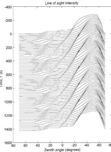
that at Ny A_{s lesund on Svalbard, roughly 2° poleward of} the ESR. At noon, during moderately intense periods of southward IMF, this station is positioned under the cusp, just poleward of the o/c field-line boundary. In mid-win-ter, and near new moon, this location is in sufficient darkness to allow measurement of the 630-nm emissions produced by atomic oxygen excited by cusp precipitation. The photometer scans the sky from the northern to the southern horizon along the magnetic meridian roughly every 20 s. Using the auroral model as described in Sect. 2.3, it is possible to reconstruct the two-dimensional dis-tribution of volume emission rate along the meridian (i.e. as a function of x and height, h). Figure 4 shows photo-meter scans, each lasting 20 s (the repeated diagonal lines), on the plot of meridional distance against time for one particular h. The plot also shows the variation of the o/c boundary and the evolution of newly opened flux regions as in Figs. 1 and 3. By integrating the airglow emission along a line of sight for each elevation angle, we have been able to generate polewards-moving events of a type that are often observed at midday in the winter by meridian scanning photometers (Sandholt et al., 1992). Figure 5 shows an example of a stack plot of predicted luminosity scans shown as a function of zenith angle with positive zenith angles being poleward, and time running down the plot. For this example, the observing site is located three degrees poleward (+"3°) of the mean location of the o/c boundary. Each polewards-moving event is caused by precipitation that results from a burst of reconnection and is thus a signature of the reconnection pulse. However, successive bursts merge into a continuous band of 630-nm emission, despite the fact that the reconnection is fully pulsed in this example. The pulsed nature of the reconnec-tion is seen in the moreconnec-tions of the equatorward boundary of the luminous band and by polewards-moving struc-tures which emerge polewards out of the continuous band.

2.6 Predictions for the ESR

Predicting how the ESR will view such polewards-moving events provides a good test for our model. In particular,

Fig. 5. Stack plot showing 630-nm luminousity observed by the meridian scanning photometer scans depicted in Fig. 4, as a function of zenith angle (positive values being northward); successive scans are shown with time running down the page

we need to know the variations in Ne and ¹e we expect to see in association with polewards-moving 630-nm events and/or stepped cusp ion precipitation. Polewards-moving structures in electron concentration have been observed by the EISCAT radar near the polar cap (Lockwood et al., 1993a). These structures were associated with a stepped ion spectrum as measured by the DMSP F10 satellite when in close conjunction. As the satellite crossed from one polewards-moving event to the next, the ion spectrum that it observed stepped to a higher energy, indicating that the field lines, and therefore the polewards-moving elec-tron concentration enhancement, were associated with two separate bursts of reconnection. The events are then seen at different stages of their evolution as discussed in Sect. 2.4. In order to predict how such events will appear in ESR data, we used the auroral model to produce outputs of Ne and ¹e as functions of ¹. The distribution of these parameters along the meridian was then modelled (as a function of x and t) and this was ‘observed’ by sampling it in the way that the ESR will when operated in a certain experiment mode. We here limited our attention, for the sake of simplicity, to an experiment in which the ESR is in the field-aligned position. The model output was integrated over 20 s, but no attempt has been made to add noise and thus limit the resolution of the output to ac-count for the signal-to-noise ratio required by the radar.

On the diagram of meridional position against time (Fig. 1), a stationary field-aligned radar beam would ap-pear as a horizontal line. What the radar sees during pulsed reconnection will depend crucially on where it is in relation to the precipitation. If the radar is positioned such that the ion-edge erodes and relaxes backwards and for-wards over it (as for the line marked ‘ESR1’ in Fig. 1), separated enhancements will be seen in Ne and ¹e. Such a case is presented in Fig. 6b, for which the radar is located at the mean latitude of the o/c boundary (+"0°), i.e. 3° equatorward of the photometer which would detect the sequence shown in Fig. 5. The electron concentration, Ne (top panel), shows a series of pulses. The concentration increases over three 20-s radar integration periods after the ion edge has eroded equatorward over the radar. This rise is caused by the rise in ¹ as the radar becomes more poleward of the ion edge (see Fig. 2 for variation of Ne with ¹ ). The decay in Ne would be instantaneous when the ion edge relaxes back in the poleward direction over the radar. However, in Fig. 6 the synthesised data are 20-s integrations and so such sudden transients tend to be smoothed. The lower panel shows ¹e; clear events of elevated electron temperature are seen at the same time as the Ne enhancements. With full transmitter power, the radar will achieve accuracies of 10% or better for both Ne and ¹e, provided that electron concentrations are high enough. Initial modelling shows that even at sunspot minimum, such resolution should be possible up to the F2 peak, if not for the full height range shown in Figs. 6 and 8. If the radar is positioned in the middle of the precipita-tion regions (represented by the line marked ‘ESR2’ in Fig. 1) it will see a continuous enhanced region where the discontinuities are much less pronounced. Variations are seen as each successive patch of newly opened flux evolves polewards over the radar beam, giving a cyclical variation of time elapsed since reconnection. An example of how Ne and ¹e would appear for such a situation is shown in Fig. 6a, for which the ESR would be 1.25° poleward of the mean location of the o/c boundary. In this case, the radar remains in the latitude band where precipitation is always present. Figure 2 shows that ¹e does not vary greatly for the 600-s period for which the precipitation is present. Thus the lower panel of Fig. 6b shows very little variation in ¹e for this case. Figure 2 shows, however, that Ne rises gradually as ¹ increases, while the precipitation persists. As a result, a cyclical variation of Ne is still seen in this case: Ne increases with ¹, but discontinuously jumps to lower values (as ¹ steps to a lower value) on the boundary between successive events.

If the radar were yet further poleward, it would cross through a region containing field lines with a longer elapsed time since reconnection (represented by the line ESR3 in Fig. 1). The example given in Fig. 6c is for the ESR +"3° poleward of the mean location of the o/c $&&&&&&&&&&&&&&&&&&&&&&&&&&

Fig. 6a–c. Plots of (top) Ne and (bottom) ¹e as a function of height and observing time, for three locations of the radar,+, measured in degrees north of the open/closed boundary, and with background reconnection rate, a"0. a +"0° gives locus ESR1 in Fig. 1b; b+"1.25° gives locus ESR2 in Fig. 1b; c+"3° gives ESR3 in Fig. 1b

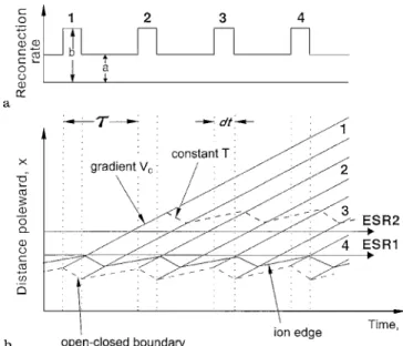
Fig. 7. Same as Fig. 1, but for a/b"0.5

boundary. The radar will still observe a continuum in the enhanced electron concentration. but in this case, the concentration gradually decays within each cycle as at these larger ¹, the precipitation has ceased, and the con-centrations are decaying (see Fig. 2). It may be difficult to detect the electron concentration fluctuations in this case, but the lower panel of Fig. 6c shows very clear fluctu-ations in ¹e. These arise because the electron temper-atures decay much more rapidly than the electron concen-tration, following the cessation of precipitation (see Fig. 2). It is important to note however, that the auroral model calculated the growth and decay of the ionospheric para-meters based on precipitation which cut off abruptly after 10 min. This cut-off will not be sharp in reality, and the resultant enhancements in electron temperature would not therefore decay so quickly. As a result, although ¹e structures may be expected on the poleward edge of the cusp, they may not be as well defined as in Fig. 6c. It is useful to compare the Ne fluctuations in the top panels in b and c of Fig. 6. The former shows rises with sudden downward jumps, whereas the latter shows falls with sudden upward jumps. The difference arises because at low ¹, Ne increases with ¹, and at high ¹ (after the precipitation has cut off) Ne decreases with ¹. Between the two will be a location where ¹ rises and then falls in each cycle, so that very little variation in Ne is seen._{The model also predicts weak enhancements in ion} temperature, ¹i, (not shown) resulting from electron-to-ion heat conductelectron-to-ion (as ¹e/¹i'1). In this work, heating effects of ionospheric flows have not been considered. Joule heating causes a rise in ion temperature, a decrease in electron concentration below the F-region peak and a redistribution of the electron concentration profile via thermal upwelling. These will effect ESR observations of not only ion temperature and electron concentration, but also electron temperature (via the energy balance criteria of an electron gas).

If IMF conditions are constant, and significant joule heating occurs, the observed effects would be seen to vary the same way in each event. This would make the events less clear in electron concentration, but would further enhance the events seen in the electron temperature.

Such effects may be significant if there is a large com-ponent of the IMF in the ½ direction, which would ini-tially give a large east/west component to the flow. This component would decay as the field lines straighten. This heating would cause an additional increase in ¹i and since it is likely that ¹i'¹e under such circumstances, ¹e may be elevated further by ion-to-electron heat conduc-tion.

3 Continuous but pulsed reconnection

The previous section considered fully pulsed reconnec-tion, with the reconnection rate between the pulses, a, equal to zero. In this section we consider pulsed, but continuous reconnection, where the background rate is half that in the pulses (a"b/2). Figure 7 corresponds to Fig. 1 for this case, in which the mean reconnection rate is now equal to 5/8b, but has the same value as in Fig. 1 (corresponding to »c"0.5 km s~1); thus b is smaller than in the previous case. Figure 7 shows that the latitudinal motions of lines of constant ¹ (e.g. the o/c boundary at ¹"0 or the ion edge at ¹+2 min) are of considerably smaller amplitude than in Fig. 1. Furthermore, the vari-ations in ¹ seen by the radar will be smaller in amplitude and without the discontinuous changes seen when a"0. Figure 8 shows the variation of Ne and ¹e predicted for a radar at a location +"3.1° poleward of the mean location of the o/c boundary. This location has been carefully selected because it corresponds to the locus ESR1 in Fig. 7 which displays the largest range of vari-ations in Ne and ¹e. The top panel shows the varivari-ations in

Ne are &10% of the peak concentration. Moving to radar

locations poleward of this (like locus ESR2 in Fig. 7) reduces these variations yet further, such that they would be undetectable. The lower panel of Fig. 8 contains the variation in ¹e which shows both rises and falls are ram-ped and without the discontinuous steps seen in Fig. 6. For most of the cusp locations, ¹e fluctuations cannot be defined, and the region at the equatorward edge where they can is very narrow in latitude in comparison with the size of the entire events.

4 Discussion

We have presented a model which has previously been used to make predictions about features seen in photo-meter and satellite data when magnetopause reconnection is pulsed, and we have applied it to observations by $&&&&&&&&&&&&&&&&&&&&&&&&&&

Fig. 8. Same as Fig. 6, but for a/b"0.5. The case shown is for

+"3.1° for which the radar follow a locus like that marked ESR1 in Fig. 7. For more poleward locations of the radar, (like ESR2 in Fig. 7), the variations in Ne and ¹e are too small to be detected

incoherent-scatter radar. The model can reproduce fea-tures such as cusp ion steps and polewards-moving 630-nm transients as a direct result of pulsing the mag-netopause reconnection rate. The purpose of this paper has been to predict the associated signature that should be detected by the new EISCAT Svalbard Radar (ESR). It has been predicted that, for a field-aligned operation of the ESR, reconnection pulses will be seen as enhance-ments in electron concentration and temperature and, to a lesser extent, ion temperature (although this latter effect will be swamped by any ion frictional heating that occurs). Whether these enhancements appear as separate events or as a continuous band, will depend on the exact position of the radar with respect to the open/closed field-line bound-ary. This model is limited by the fact that, at present, it is only possible to calculate the effect of electron precipita-tion. Ion precipitation is likely to be significant in altering the intensity of the enhancements, however, cusp ion pre-cipitation is a strong function of elapsed time since recon-nection and thus its effects should serve to magnify the effects predicted here. On the other hand, the one-dimen-sional nature of the auroral model used means that the thermospheric winds (which will not, in general, match the plasma convection) are likely to smear the 630-nm optical events. This is not a problem for the ESR measurements predicted here, as the thermospheric wind has little or no bearing on the modelled ionospheric electron temperature and concentration enhancements.

The modelling indicates that pulsed reconnection will be very difficult to detect if the reconnection rate within the pulses (b) is less than about twice the value between the pulses (a). Figure 8 does show clear cyclical variations in ¹e fora"b/2, but these are only found in a very narrow band of latitudes at the equatorward edge of the cusp. We can quantify the width of this band, Dx. From our as-sumption that »c is constant, we obtain the expression

Dx"(b!a) (1!(dt/q) dt), where, as before, q is the pulse

repetition period, dt is the duration of enhanced reconnec-tion in each cycle and a and b are the background and enhanced reconnection rates, respectively. In the above case, with a/b"1/2, »c"500 m s~1, dt"1 min and q"4 min, Dx"18 km. This can be compared with the same case but with a"0 (fully pulsed reconnection), for whichDx"90 km. Even for fully pulsed reconnection, the pulses may be difficult to detect if the radar is near the centre of the latitude range covered by the cusp ion pre-cipitation.

In all cases shown here, the mean latitude of the o/c boundary has not drifted relative to the radar. In reality, the boundary is always likely to be moving over the radar. For example, the 630-nm transients are observed usually during southward IMF and when the cusp/cleft red line aurora is migrating equatorwards because of erosion of the dayside magnetosphere (Fasel, 1995; Sandholt et al., 1992). Thus for fully pulsed reconnection, the Ne and ¹e pulses shown in Fig. 6a may rapidly evolve to a form like those in Fig. 6b and then those in 6c. Such changes will make identification of the pulses yet more difficult. Never-theless, with satellite, optical measurements and the ESR, the effects of many different reconnection patterns can now be studied in detail, and we look forward to testing

our model further and interpreting the results, using the first data from the ESR.

Acknowledgements. This work was supported by the UK Particle

and Astronomy Research Council.

Topical Editor D. Alcayde´ thanks A. Rodger and N. Cornilleau-Wehrln for their help in evaluating this paper.

References

Burch, J. L., Quasi-neutrality in the polar cusp, Geophys. Res. ¸ett., 12, 469—472, 1985.

Carlson, H. G., and A. Egeland, Introduction to Space Physics, chapter 14, pages 459—502. Cambridge University Press, 1995. Coroniti, F., and C. Kennel, Can the ionosphere regulate

magneto-spheric convection? J. Geophys. Res., 78, 2837— 2851, 1973. Cowley, S. W. H., The causes of convection in the Earth’s

magneto-sphere — a review of developements during the IMS, Rev.

Geo-phys., 20, 531—565, 1982.

Cowley, S. W. H., A. P. V. Eyken, F. C. Thomas, P. J. S. Williams, and D. M. Willis, Studies of the cusp auroral zone with incoher-ent-scatter radar — the scientific and technical case for a polar cap radar, J. Atmos. ¹err. Phys., 52, 645—663, 1990.

Cowley, S. W. H., M. P. Freeman, M. Lockwood, and M. F. Smith, The ionospheric signature of flux transfer events, in Cluster

dayside polar cusp, number ESA SP-330 in ESA SP, ESA

publica-tions, ESTEC Noordwijk, pages 105—112, 1991.

Etemadi, A., S. W. H. Cowley, D. M. W. M. Lockwood, B. J. I. Bromage, and H. Lu¨hr, The dependence of high-latitude dayside ionospheric flows on the north-south component of the IMF, a high time resolution correlation analysis using EISCAT ‘‘po-lar’’ and AMPTE UKS and IRM data, Planet. Space Sci., 36, 471, 1988.

Fasel, G. J., Dayside poleward-moving auroral forms: a statistical study, J. Geophys. Res., 100, 11891—11905, 1995.

Hedin, A. E., Extension of the MSIS thermosphere model into the middle and lower atmosphere, J. Geophys. Res., 96, 1159—1172, 1991.

Holzer, T. E., and G. C. Reid, The response of the dayside magneto-sphere-ionosphere system to time-varying field-line reconnec-tion, J. Geophys. Res., 80, 2041—2049, 1975.

Lockwood, M., Ground-based and satellite observations of the cusp: Evidence for pulsed magnetopause reconnection, in Physics of

the magnetopause, eds. Song, P., B. U. O. Sonnerup, and M.

Thomsen, volume 90, pages 417—426. American Geophysical Union Monograph, 1995a.

Lockwood, M., The location and characteristics of the reconnection X-line deduced from low-altitude satellite and ground-based observations: 1. theory. J. Geophys. Res., 100, 21791—21802, 1995b.

Lockwood, M., and S. W. H. Cowley, Ionospheric convection and the substorm cycle, in Substorms 1, Proceedings of the First

Interna-tional Conference on Substroms, ICS-1, ed. C. Mattock,

ESA-SP-335, pages 99—110, Nordvijk, The Netherlands, European Space Agency, European Space Agency Publications, 1992.

Lockwood, M., and C. J. Davis, The occurrence probability, width and number of steps of cusp precipitation for fully-pulsed recon-nection at the dayside magnetopause, J. Geophys. Res., 100, 7627—7640, 1995.

Lockwood, M., and M. F. Smith, Low- and mid-altitude cusp par-ticle signatures for general magnetopause reconnection rate vari-ations: I—theory. J. Geophys. Res., 99, 8531—8555, 1994. Lockwood, M., and M. N. Wild, On the quasi-periodic nature of

magnetopause flux transfer events, J. Geophys. Res., 98, 5935—5940, 1993.

Lockwood, M., W. F. Denig, A. D. Farmer, V. N. Davda, S. W. H. Cowley, and H. Lu¨hr, Ionospheric signatures of the pulsed recon-nection at the Earth’s magnetopause, Nature, 361, 424—427, 1993a.

Lockwood, M., J. Moen, S. W. H. Cowley, A. D. Farmer, U. P. Løøvhaug, H. Lu¨hr, and V. N. Davda, Variability of dayside convection and motions of the dayside cusp/cleft aurora,

Geo-phys. Res. ¸ett., 20, 1011—1014, 1993b.

Lockwood, M., T. G. Onsager, C. J. Davis, M. F. Smith, and W. F. Denig, The characteristics of the magnetopause reconnection x-line deduced from low-altitude satellite observations of cusp ions, Geophys. Res. ¸ett., 21, 2757—2760, 1994.

Lummerzheim, D., Electron transport and optical emissions in the

aurora, PhD thesis, University of Alaska, Fairbanks, 1987.

Newell, P. T., W. J. Burke, C. I. Meng, E. R. Sanchez, and M. E. Greenspan, Identification and observation of the plasma mantle at low altitude, J. Geophys. Res., 96, 35—45, 1991.

Palmer, J. R., Plasma density variation in the aurora, PhD thesis, The University of Southampton, 1995.

Pinnock, M., A. S. Rodger, J. R. Dudeny, K. B. Baker, P. T. Newell, R. A. Greenwald, and M. E. Greenspan, Observations of an enhanced convection channel in the cusp ionosphere, J. Geophys.

Res., 98, 3767—3776, 1993.

Pinnock, M., A. S. Rodger, J. R. Dudeney, F. Rich, and K. B. Baker, High spatial and temporal resolution observations of the iono-spheric cusp, Ann. Geophysicae, 13, 919—925, 1995.

Rees, M. H., Antarctic upper-atmosphere investigations by optical methods, Planet. Space Sci., 37(8), 955—966, 1989.

Rees, M. H., and D. Lummerzheim, Characteristics of auroral elec-tron precipitation derived from optical spectroscopy, J. Geophys.

Res., 94(NA6), 6799—6815, 1989.

Reiff, P. H., T. W. Hill, and J. L. Burch, Solar wind plasma injection at the dayside magnetospheric cusp, J. Geophys. Res., 82, 479— 491, 1977.

Rishbeth, H., and P. J. S. Williams, The EISCAT ionospheric radar: the system and its early results, Q. J. R. Astron. Soc., 26, 478—512, 1985.

Rosenbauer, H., H. Grunwaldt, M. D. Montgomery, G. Paschmann, and N. Skopke, HEOS-2 plasma observations in the distant polar magnetosphere: the plasma mantle, J. Geophys. Res., 80, 2723—2737, 1975.

Sanchez, E. R., G. L. Siscoe, and C.-I. Meng, Inductive attenuation of the transpolar voltage, Geophys. Res. ¸ett., 18, 1173—1176, 1991.

Sandholt, P. E., M. Lockwood, W. F. Denig, R. C. Elphic, and S. Leontjev, Dynamical auroral structure in the vicinity of the polar cusp: multipoint observations during southward and northward IMF, Ann. Geophys., 10, 483—497, 1992.

Shelley, E. G., R. D. Sharp, and R. G. Johnson, He`` and H` flux measurements in the dayside magnetospheric cusp, J. Geophys.

Res., 81, 2363, 1976.

Todd, H., S. W. H. Cowley, M. Lockwood, D. M. Willis, and H. Lu¨hr, Response time of the high-latitude dayside ionosphere to sudden changes in the north-south component of the IMF, Planet. Space

Sci., 36, 1415—1428, 1988.