Assessing heterogeneity in transition propensity in multistate capture-recapture data

HAL Id: hal-02387535

https://hal.archives-ouvertes.fr/hal-02387535

Submitted on 30 Jan 2020

HAL is a multi-disciplinary open access

archive for the deposit and dissemination of

sci-entific research documents, whether they are

pub-lished or not. The documents may come from

teaching and research institutions in France or

abroad, or from public or private research centers.

L’archive ouverte pluridisciplinaire HAL, est

destinée au dépôt et à la diffusion de documents

scientifiques de niveau recherche, publiés ou non,

émanant des établissements d’enseignement et de

recherche français ou étrangers, des laboratoires

publics ou privés.

Assessing heterogeneity in transition propensity in

multistate capture-recapture data

Anita Jeyam, Rachel S. Mccrea, Roger Pradel

To cite this version:

Anita Jeyam, Rachel S. Mccrea, Roger Pradel. Assessing heterogeneity in transition propensity in

multistate capture-recapture data. Journal of the Royal Statistical Society: Series C Applied Statistics,

Wiley, 2020, 69 (2), pp.413-427. �10.1111/rssc.12392�. �hal-02387535�

© 2019 The Authors Journal of the Royal Statistical Society: Series C (Applied Statistics) Published by John Wiley & Sons Ltd on behalf of the Royal Statistical Society.

This is an open access article under the terms of the Creative Commons Attribution License, which permits use, distribution and reproduction in any medium, provided the original work is properly cited.

0035–9254/20/69000

Assessing heterogeneity in transition propensity in

multistate capture–recapture data

University of Kent, Canterbury, UK

and Roger Pradel

Centre d’Ecologie Functionelle et Evolutive, Montpellier, France [Received September 2018. Final revision November 2019]

Summary. Multistate capture–recapture models are a useful tool to help to understand the

dynamics of movement within discrete capture–recapture data.The standard multistate capture– recapture model, however, relies on assumptions of homogeneity within the population with respect to survival, capture and transition probabilities. There are many ways in which this model can be generalized so some guidance on what is really needed is highly desirable. Within the paper we derive a new test that can detect heterogeneity in transition propensity and show its good power by using simulation and application to a Canada goose data set. We also demonstrate that existing tests which have traditionally been used to diagnose memory are in fact sensitive to other forms of transition heterogeneity and we propose modified tests which can distinguish between memory and other forms of transition heterogeneity.

Keywords: Diagnostics; Goodness of fit; Markovian transitions

1. Introduction

Simple capture–recapture studies collect binary information of capture or non-capture of marked individuals over a series of discrete occasions, yielding a capture history for each individual ob-seved within the study. The associated Cormack–Jolly–Seber model enables the estimation of survival and capture probabilities from such data. It is limited in its biological scope because it utilizes only the information of whether the animal is captured or not (Lebreton et al., 2009). But ecologists can be interested in aspects such as the geographic location for migratory birds, or their breeding status. Such information is easily collected on the animals’ capture and recorded as states.

States were defined by Lebreton and Pradel (2002) as ‘any mutually exclusive and identifiable events in the life cycle of the population under study’. They can be static, in which case they remain the same throughout the individual history (e.g. sex). States can also be dynamic, in which case they either follow a deterministic (e.g. age) or stochastic (e.g. health status) process. For static and deterministic states, information is available as long as the animal is captured at least once (Lebreton et al., 2009). The general definition of states enables multistate models to tackle a large array of biological questions; they also have the ability to handle the more complex stochastic dynamic states.

Address for correspondence: Rachel McCrea, School of Mathematics, Statistics and Actuarial Science, Univer-sity of Kent, Cornwallis Building, Canterbury, Kent, CT2 7NF, UK.

The information of interest is collected when the animal is captured, resulting in individ-ual capture histories. For the Cormack–Jolly–Seber framework captures and non-captures are recorded as 1s and 0s respectively. For the multistate setting the 1s are replaced by the state in which the animal is captured. For example A B 0 C C codes the information: ‘captured at occasion 1 in state A, recaptured at 2 in B, not captured at 3 and recaptured in C at 4 and 5’. The data may be summarized by a multistatem-array, where m_ij.r, s/ denotes the number of individuals that are captured in stater at occasion i and next captured at occasion j in state s; Ri.r/ denotes the number of individuals that are released at occasion i in state r and vi.r/ denotes the number of individuals that were seen for the last time at occasioni in state r (McCrea and Morgan (2014), page 88).

The Arnason–Schwarz model (Arnason, 1972, 1973; Schwarz et al., 1993) is the direct mul-tistate extension of the Cormack–Jolly–Seber model (Pradel et al., 2003). It is conditional on the first release of individuals and relies on the assumption of homogeneity of the survival and recapture probabilities, for all animals in a given stater. Thus, all animals in state r at time i are assumed to have an equal probability of surviving from occasioni to i + 1, and it is denoted byφr_i. Note that this survival probability represents ‘apparent’ survival as without additional information death is confounded with permanent emigration. All animals in stater at time i are also assumed to have the same recapture probability, denoted bypr_i.

Furthermore, multistate models also involve transition or movement probabilities between states; these are denoted byψ_irsand represent the probability of moving to states by occasion i+1 for an animal in state r at time i, conditionally on the animal being alive and in the study area at occasioni + 1. The processes of survival and transition are separated under the assumption that survival depends only on the state of the animal at timei, i.e. animals survive first and then move. Animals in a given state at a given occasion are assumed also to have homogeneous behaviour in terms of transitions; the process governing the transition between states is assumed to be first-order Markovian, i.e. the future state depends only on the current state.

Due to the complex nature of multistate capture–recapture models, possible departures from model assumptions are numerous. Pradel et al. (2003) derived goodness-of-fit tests for multistate capture–recapture models through the factorization of the likelihood function and evaluation of Pr.data|m/ (where m denotes a set of sufficient statistics for the Arnason–Schwarz model), which can be used to assess model adequacy. This function was further partitioned into conditionally independent terms which can be used to diagnose different causes of departure from model assumptions separately. The component tests have been used to detect memory, transience and trap effects and the form and power of these existing tests are described in Section 2.

The importance of accounting for individual variation in capture and demographic processes has been well documented; see for example Gimenez et al. (2018a) for a recent review. However, the investigation of transition heterogeneity has been limited to the modelling of memory within a study species (Rouan et al., 2009). The importance of geographical variation in distinct sub-populations has been detected in recent capture–recapture studies; see for example Chabanne

et al. (2017).

The work of this paper was motivated by the desire to be able to detect mover–stayer behaviour in animal populations. The mover–stayer structure was first introduced in social studies, to de-scribe different patterns of industrial mobility (see for example Spilerman et al. (1972)). It was originally defined as the existence of two types of individuals: some who stay where they are and others who move homogeneously. We define it more loosely here as some individuals being more likely to move (movers) than others (stayers). We assume that this behaviour is an intrin-sic characteristic of the animals and therefore does not change over time. This phenomenon has rarely been analysed in a capture–recapture framework but could provide new insight into

biological processes such as migration patterns or stages of disease progression. Indeed, hetero-geneous dispersal has been found in ungulates (Shafer et al., 2011) and birds (Gillingham et al., 2013), whereas ‘heterogeneity in susceptibility and infectivity is inherent to infectious disease transmission in nature’ (Rodrigues et al., 2009).

Models accounting for heterogeneity in transition, mover–stayer structure or memory are challenging to fit (Rouan et al., 2009), and therefore it is desirable to diagnose these departures from basic model assumptions before any model fitting. Modelling approaches which relax the first-order Markovian approaches include a conditional likelihood approach to incorporate a second-order Markovian process (Hestbeck et al., 1991; Brownie et al., 1993) and a semi-Markov Arnason–Schwarz model which enables the estimation of a dwell time distribution for state retention (King and Langrock, 2016).

We define a new test which can detect heterogeneity in transition probabilities in Section 3 and evaluate both existing and new approaches by using simulation in Section 4. Following the results of the simulation study we present an adaptation of the existing test of memory (test WBWA) (Pradel et al., 2003) which together with the new test enables us to differentiate the property of memory from other forms of heterogeneity. The tests that are examined in this paper are then applied, in Section 5, to a Canada geese, Branta canadensis, data set (Hestbeck et al., 1991; Brownie et al., 1993). Finally we conclude with a discussion in Section 6.

The data that are analysed in the paper and the programs that were used to analyse them can be obtained from

https://rss.onlinelibrary.wiley.com/hub/journal/14679876/series-c-datasets.

2. Existing tests for transition behaviour

Within this section we outline the existing suite of diagnostic tests derived for multistate mod-els (Pradel et al., 2003). These tests are based on the Jolly movement model, rather than the Arnason–Schwarz model, because of the requirements for the theoretical derivation of the tests. The Jolly movement model differs only slightly from the Arnason–Schwarz model, with the capture probabilities depending not only on the state in which the animal is captured, but also on its previous state. The multisite analogues of the single-site tests 2 and 3 that were proposed in Burnham (1991) are test M and test 3G respectively. Test M contrasts individuals that are not caught at a given occasion (yet which are known to be alive and are recaptured later in the study) with those caught at the same occasion. Thus test M can diagnose whether trap dependence is exhibited in the data. Test 3G investigates the effect of the past capture history on their future, for animals captured and released at the same time and state. Test 3G is further partitioned into components that are used to detect memory (test WBWA) and transience (test 3G.SR).

The sum of these component multistate tests can be used to estimate an overdispersion coef-ficient which can be used to adjust information criteria model selection to account for lack of fit (Pradel et al., 2005). The tests for multistate capture–recapture data have therefore been used for a wide range of ecological applications, e.g. for the evaluation of reproductive costs of swallows (Schaub and von Hirschheydt, 2009), understanding of temporal and spatial variation in a turtle population (Roe et al., 2009), migration in whale populations (Gowan et al., 2019) and estimation of the dynamic drivers of recruitment for bird species (Crespin et al., 2006; Henaux et al., 2007). Test WBWA is the only diagnostic test which examines the transitions that are exhibited by individuals in the population and it is therefore that test which we examine more closely here. Test WBWA assesses whether animals are more likely to be next re-encountered in the same

Table 1. Contingency table of data for components of diagnostic test WBWA.i, r/

Last seen in Next seen in A : : : Next seen in K A ΣT_h=i+1m_{A}i,h.r, A/ : : : ΣT_h=i+1m_{A}i,h.r, K/ ::

:

K ΣT_h=i+1m_{K}i,h.r, A/ : : : ΣT_h=i+1m_{K}i,h.r, K/

state as the state that they were last seen in. The test is decomposed into components which condition on individuals who are captured in stater at occasion i. The null hypothesis for this component test is

‘For animals encountered in stater at occasion i, there is no difference in the expected state of next re-encounter between the animals last seen in the different states’

(Choquet et al., 2009). The alternative hypothesis is defined as

‘For animals encountered in a given state r at a given occasion i, the probability of being next re-encountered in the same state as the one they were last seen in is higher than the probability of being next re-encountered in other states’.

Suppose that the system hasK discrete states and there are T capture occasions during the study. Extending the standard sufficient statistics that were introduced earlier, we letm_{0}ij.r, s/ denote the number of new individuals released in stater at occasion i and next recaptured in states at occasion j and let m_{q}ij.r, s/ denote the number of individuals released in state r at occasioni and next recaptured in state s at occasion j and which were captured before occasion i in stateq. The contingency table of data that is required to perform component test WBWA.i, r/ is presented in Table 1. The tests that are performed on the contingency tables are the usual

χ2_{-tests of independence (or Fisher’s exact test is used in cases of small numbers) and to obtain} the global test statistic the independent component tests are summed as are the associated degrees of freedom to calculate the significance of test WBWA.

Alternatively, Pradel et al. (2005) proposed to use Cohen’sκ to detect memory. Cohen’s κ is typically used as a measure of agreement between two raters classifying subjects according to the same scale, taking into account the agreement that can occur by chance; it is applied to data formatted as a square contingency table (Everitt (1992), page 146). In the memory context,κ is used to measure the agreement between the previous and future state for animals that are seen at occasioni in a given state r. It is applied to the square K ×K contingency table WBWA.i, r/ that is presented in Table 1. Leta_bsdenote the cell frequencies of table WBWA.i, r/, a_b:the row sums and a:sthe column sums, andn the total number of animals in the contingency table. The proportion of agreement that is observed is derived from the diagonal elements of the table:PA=ΣK_i=1aii=n. The proportion of agreement that may occur by chance is computed from the row and column sums:PC= {.ΣK_i=1ai:a:i/=n}n. Finally, Cohen’s κ is defined as κ = .PA− PC/=.1 − PC/ (Everitt (1992), page 148).

3. New testing approaches

The existence of a mover–stayer structure in the population lends itself naturally to an extension of the test of positive association that was developed for the detection of capture heterogeneity

(Jeyam et al., 2018). Indeed, if the pair being examined is composed of two movers or two stayers, the probability of having a discordant pair is the same as that of a concordant pair: no individual has a higher probability of moving than the other and the intensity of movement before and after the middle observation is unrelated. But, when the pair consists of a stayer and a mover, the mover tends to have made more movements before as well as after the middle observation (concordant pair). Because of the presence of these latter pairs, overall we expect an excess of concordant pairs. When individuals are not captured we do not know what state they are in. Therefore when we construct the test we condition on capture. Because the test makes use of observations of live individuals, no assumption is required on the relative survivorship and detectability of movers and stayers. Within the simulation in Section 4 we demonstrate that this does not adversely affect the performance of the test even when capture probabilities are state dependent. Unlike the diagnostic tests that were described in the previous section the test that we derive here requires the full encounter history of each individual rather than them-array sufficient statistics.

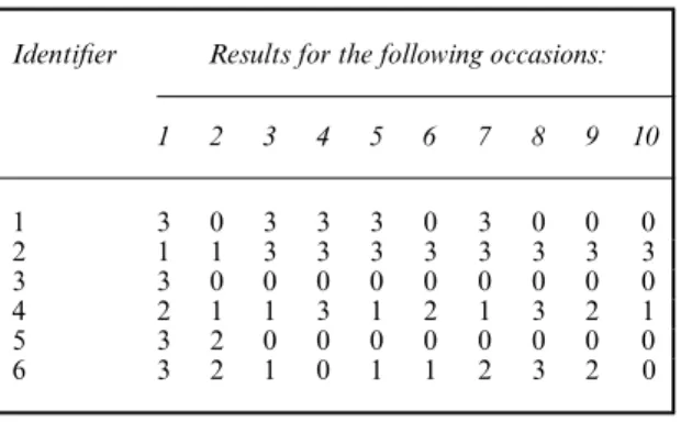
Some example multistate capture histories are presented in Table 2. Consider the non-zero part of an individual encounter history and let the middle occasion of non-zero encounters be denoted byτ. The capture histories are then grouped by state in which the animal is captured at occasionτ to reduce potential noise due to state-specific properties of the animals. For an individual encounter history to contribute to the test they must have at least one informative encounter on each side ofτ, so animals must have been captured at least three times. The num-ber of observed movements between first-release occasion andτ and the number of observed movements betweenτ and the last capture occasion are counted. To standardize this informa-tion, we compute the proportion of previous and future movements, using as the denominator the maximum number of previous or future possible movements conditional on capture, i.e. the maximum number of previous or future movements that we could potentially observe. Finally, the ranks of these proportions are used to represent the intensity of movement of the animals relative to one another, with the lowest rank denoting the least movement and the highest the most movement. We present a worked example of test construction in Table 3, based on the example capture histories that are presented in Table 2. Note that animals with identifiers 3 and 5 are not used for the test because they are captured fewer than three times.

The range of ranks is limited and many ties are expected, so Goodman–Kruskal’sγ is used as a measure of positive association between previous and future movements. Theγ-measure is estimated, based on the numbers of discordantD and concordant C pairs observed: ˆγ = .C −D/=.C +D/. A pair of observations is concordant if the observation which ranks higher or lower for the previous encounter also ranks respectively higher or lower for the future encounter.

Table 2. Example capture histories

Identifier Results for the following occasions:

1 2 3 4 5 6 7 8 9 10 1 3 0 3 3 3 0 3 0 0 0 2 1 1 3 3 3 3 3 3 3 3 3 3 0 0 0 0 0 0 0 0 0 4 2 1 1 3 1 2 1 3 2 1 5 3 2 0 0 0 0 0 0 0 0 6 3 2 1 0 1 1 2 3 2 0

Table 3. Example capture histories: extracting the information required for the positive association test by state at the middle occasion†

Identifier Non-zero capture history Results for previous Results for future

movements movements

NM max pr r NM max pr r

State 1

6 3 2 1 1 1 2 3 2 2 3 2/3 1 3 4 3/4 1

4 2 1 1 3 1 2 1 3 2 1 3 4 3/4 2 5 5 1 2

State 2: no capture histories State 3

1 3 3 3 3 3 0 2 0 1 0 2 0 1

2 1 1 3 3 3 3 3 3 3 3 1 4 1/4 2 0 5 0 1

†The middle occasion is denoted in italics for each capture history. NM denotes the number of movements, max the maximum possible number of observed movements, pr the proportion andr the rank.

Conversely a pair of observations is discordant if the observation which ranks higher or lower for the previous encounter ranks respectively lower or higher for the future encounters.

We expect a high number of concordant pairs for a mover–stayer structure and hence use a one-sided test. The test statistic that is used isz_s=γ_s=√var.γ_s/, where s denotes the state in which the animal is in at the middle occasion. We investigated both the conservative version of the test and the Brown and Benedetti (1977) version. To be conservative regarding the distributional approximation of the test statistic, the number of animals that are used for the test at each state was required to be at least 30 for the test to be applicable. For the worked example that is presented in Table 3, theγ-estimate is not applicable for state 2 as there are no capture histories with state 2 at the middle occasion, and state 3 which presents only one tied pair. The individuals in state 1 form a concordant pair.

We investigated various versions of a positive association test between ranks of previous movements and ranks of future movements, split by state. Firstly, we used the animals with at least one informative movement on each side of the middle occasion, i.e. captured at least three times and secondly imposing the constraint of at least two informative movements on each side of the middle occasion, i.e. captured at least five times.

Further, we also investigated the performance of two global versions of the test per state: a test over all states using the middle occasion of the capture histories, without grouping the data by state, which we expected to be sensitive to state-specific properties and, thus, non optimal and also a summary test over the states, based on the standardized sum of the independent test statistics obtained from the test by state, withK denoting the number of states: z_G=ΣK_s=1z_s=√K.

4. Simulation evaluation

Different scenarios were explored to assess the performance of the various versions of the test. For each simulation 250 data sets of 2500 animals were simulated, with 10 capture occasions (250 animals released per occasion) and three live states, all equally likely to be the state at first capture. We note that individuals that are released in later cohorts will not contribute to the test statistic since individuals must have been captured at least three times. The survival probability was constant over time and states, and set toφ=0:9 for all scenarios. The capture probability was

set top=0:9, constant over times and states for most scenarios. We also explored lower capture probability scenarios (denoted bypL), state (ps) or time-dependent (pt) capture probabilities and their detailed values are given further in the text, in the relevant sections.

First, we simulated simple homogeneous scenarios: (a) M, all animals tend to move;

(b) MO, a more extreme situation with a zero probability of remaining in the same state; (c) S, animals tend to remain where they were;

(d) P, preference for one state—e.g. a very high probability of moving to or remaining in state 2;

(e) A, avoidance of one state—e.g. a very high probability of moving from state 2; (f) SD1 and SD2, strongly state-dependent transition probabilities.

All these homogeneous scenarios constituted controls, which were used to check the type I error rate. The transition matrices for these homogeneous scenarios are detailed in the web Table 1. Further, we investigated heterogeneous scenarios with two groups of animals per data set presenting different behaviours in terms of transitions:

(a) MS1 and MS2, mover–stayer structure with different proportions of stayers (π1= 0:3 under MS1 andπ1= 0:7 under MS2);

(b) P2G, animals preferring different states—e.g. one group preferring state 1; the other state 2;

(c) A2G, animals avoiding different states—e.g. one group avoids state 1 whereas the other avoids state 2;

(d) HM, heterogeneity in movement—e.g. animals had different movement patterns but had the same rate of movement (and therefore were not within the mover–stayer sce-nario).

Apart from the mover–stayer scenarios, the heterogeneous scenarios were simulated with an equal proportion of animals from each group (π1= 0:5). The transition matrices for each of these scenarios are presented in web Table 2. In addition to these heterogeneous scenarios, the more complex memory phenomenon was also examined in scenario Mem. For this scenario, the probability of being ati + 1 in the same state as at i − 1 is higher than others. The transition matrices generating the data sets with memory under both scenarios considered are presented in web Table 3. All these scenarios constitute violations of the multistate model assumption of homogeneity in transitions; and their objective was to assess the specificity of the test of positive association to a mover–stayer structure. Finally, for some of the scenarios, we exam-ined the potential effect of state-dependent capture probabilities (settingp1=0:9, p2=0:35 and p3_{=0:7 with the superscripts corresponding to the states), lower capture probability .p=0:5/ or} slightly time-dependent probabilities. These scenarios were respectively denoted by subscripts ps, pLort.

4.1. Main results

4.1.1. Test of positive association

In this section, we present the results that were obtained by using two versions of the conservative positive association test split by state (simple upper bound for variance estimate): based on one informative movement on each side (i.e. animals captured at least three times) in Table 4 and based on two informative movements on each side in Table 5 (i.e. animals captured at least five times). In Tables 4 and 5 we also present the results that were obtained by using the summary test based on both versions of the test by state. All the versions of the test were coded by using

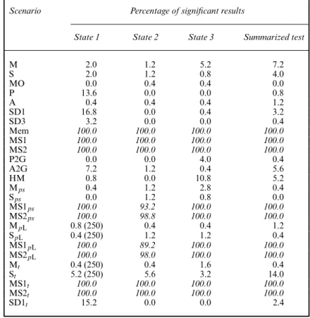
Table 4. Test of positive association (conservative variance estimate), split by state†

Scenario Percentage of significant results

State 1 State 2 State 3 Summarized test

M 2.0 1.2 5.2 7.2 S 2.0 1.2 0.8 4.0 MO 0.0 0.4 0.4 0.0 P 13.6 0.0 0.0 0.8 A 0.4 0.4 0.4 1.2 SD1 16.8 0.0 0.4 3.2 SD3 3.2 0.0 0.0 0.4 Mem 100.0 100.0 100.0 100.0 MS1 100.0 100.0 100.0 100.0 MS2 100.0 100.0 100.0 100.0 P2G 0.0 0.0 4.0 0.4 A2G 7.2 1.2 0.4 5.6 HM 0.8 0.0 10.8 5.2 Mps 0.4 1.2 2.8 0.4 Sps 0.0 1.2 0.8 0.0 MS1_ps 100.0 93.2 100.0 100.0 MS2ps 100.0 98.8 100.0 100.0 M_pL 0.8 (250) 0.4 0.4 1.2 S_pL 0.4 (250) 1.2 1.2 0.4 MS1_pL 100.0 89.2 100.0 100.0 MS2_pL 100.0 98.0 100.0 100.0 Mt 0.4 (250) 0.4 1.6 0.4 S_t 5.2 (250) 5.6 3.2 14.0 MS1t 100.0 100.0 100.0 100.0 MS2t 100.0 100.0 100.0 100.0 SD1t 15.2 0.0 0.0 2.4

†One informative movement (animal captured at least three times); percentage of significant results (number of applicable tests); high percentages of significant results (greater than 50%) are in italics.

R (R Core Team, 2017). The results are presented in terms of the percentage of significant test results, using a level of significance of 5%.

Both the one- and the two-informative-movement tests have a very high power to detect a mover–stayer structure. Table 4 shows that, when one informative movement is used, 100% of the results for the tests split by state are significant for scenarios MS1 and MS2 as well as MS1_t and MS2_t, and around 90–100% for the versions of these scenarios with a state-dependent or lower capture probability. However, it is slightly too sensitive in some of the control situations (e.g. 16.8% for SD1, state 1, and 13.6% for P, state 1) and it does not enable us to distinguish a mover–stayer structure from short-term memory, which also results in 100% of significant results, for both Mem1 and Mem2.

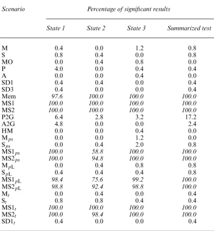
When using two informative movements (see Table 5), the type I error is under 5% for all control scenarios. Again, around 100% of the results for the tests split by state are significant for scenarios MS1 and MS2 as well as MS1_t and MS2_t; the same is observed for most of the mover–stayer scenarios with a state-dependent or lower capture probability. Among the other heterogeneity scenarios that were considered, the test does not react in most cases; it is slightly sensitive only to heterogeneity in preference (6.4% for state 1) but, like the test using one informative movement, it is extremely sensitive to memory.

Table 5. Test of positive association (conservative variance estimate), split by state†

Scenario Percentage of significant results

State 1 State 2 State 3 Summarized test

M 0.4 0.0 1.2 0.8 S 0.8 0.4 0.0 0.8 MO 0.0 0.4 0.8 0.0 P 4.0 0.0 0.4 0.4 A 0.0 0.0 0.4 0.0 SD1 0.4 0.4 0.0 0.4 SD3 0.4 0.0 0.0 0.4 Mem 97.6 100.0 100.0 100.0 MS1 100.0 100.0 100.0 100.0 MS2 100.0 100.0 100.0 100.0 P2G 6.4 2.8 3.2 17.2 A2G 4.8 0.0 0.0 2.4 HM 0.0 0.0 0.4 0.0 Mps 0.0 0.0 1.2 0.0 Sps 0.0 0.4 2.0 0.8 MS1_ps 100.0 58.8 100.0 100.0 MS2ps 100.0 94.8 100.0 100.0 M_pL 0.0 0.4 0.8 0.8 S_pL 0.4 0.4 0.4 0.8 MS1_pL 98.4 75.6 99.2 100.0 MS2_pL 98.8 92.4 98.8 100.0 Mt 0.0 0.4 0.0 0.4 S_t 0.8 0.8 0.4 0.4 MS1t 100.0 100.0 100.0 100.0 MS2t 100.0 98.4 100.0 100.0 SD1t 0.4 0.0 0.0 0.4

†Two informative movements (animal captured at least five times); percentage of significant results (number of applicable tests); high percentages of significant results (greater then 50%) are in italics.

The results that are presented in the final columns of Tables 4 and 5 show that the summarized test presents the same characteristics: very powerful at detecting a mover–stayer structure and also very sensitive to memory (100% of significant results for all situations, whether one or two informative movements are used). Note that the control data sets present a type I error that is lower than 5% (apart from M: 7.2% when only one informative occasion is used). This is an expected result as the test is conservative. Both versions of the summarized tests do not react to most of the other scenarios of heterogeneity, apart from heterogeneity in preferences scenario P2G, 17.2% for the test using two informative movements, whereas the summarized test with one informative movement is affected by time dependence for scenario S_t, 14.0% of significant results. Since short-term memory is a more local phenomenon than the mover–stayer behaviour, we attempted to use animals with at least three informative previous and future movements (animals captured at least seven times). However, this resulted in a very high loss of data (only 150 animals used on average per data set, out of 2500) while only marginally decreasing the sensitivity of the test to memory. The percentages of significant results obtained were respectively, for states 1, 2 and 3, 48.4% (250), 92% (250) and 92% (250) for scenario Mem.

The loss in data resulting from using animals with at least two or three informative movements is not outweighed by any significant gain in terms of identifying the mover–stayer structure

separately from memory. At this stage, the summarized test using animals with at least one informative previous and future movement seems to be the preferred option.

The results from the global test that was performed using the middle occasion without prior grouping of the animals by their state at that occasion are not presented here because of the test’s poor performance. Indeed it reacted strongly to control scenarios such as state-dependent transition scenario SD1 (54.4% using two informative movements; 80% using only one). Hence this test was not adequate for our objective.

Likewise, the results of the tests version using the Brown and Benedetti (1977) estimates are not presented in this paper, although they were investigated. Again, these tests were sensitive to phenomena other than mover–stayer and memory. e.g. 56.8% of significant results for ho-mogeneous scenario SD1, for state 1, when using the test split by state with one informative movement and 27.6% for the summarized test, and 54.4% for the summarized test for scenario P2G, using two informative movements.

4.1.2. Existing memory tests

We investigated the tests that are currently used to detect memory, to assess whether they were actually specific to memory. For these tests, time-dependent scenarios were not considered since the tests are based on independent components by state at each occasion. Test WBWA was coded by adapting MATLAB code provided by R. Choquet, which is now available in the R package R2Ucare (Gimenez et al., 2018b), we used the Kappa function from R package vcd to obtain theκ-estimate, its asymptotic standard error and the resulting z-statistic (Meyer et al., 2006). We used both a one-sided test corresponding toκ > 0 (more agreement than expected by chance, which is the case for memory) and a two-sided test which also adds to the alternative

κ < 0 (less agreement than expected by chance, which would correspond to animals avoiding

the site where they were last seen) (see for example Everitt (1992), page 148).

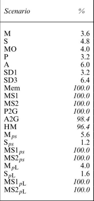
Table 6 showed that the global WBWA test (formed by summing the WBWA tests by occasion and state) reacts strongly not only to memory, but also to the existence of a mover–stayer structure, heterogeneity in preferences or avoidance as well as heterogeneity in movement, with close to 100% of significant results for all these situations. We also considered the component tests split by state and occasion and, as expected, the split WBWA test shows similar reactions to those of the global test, though not always as strong or for all states.

The results that were obtained by using theκ-statistic are very similar to the results that were obtained with test WBWA: the test reacts strongly to both memory and a mover–stayer structure; it is also sensitive to two groups with different preferences and to heterogeneity in movement. Because of the similarities between the results from test WBWA and Cohen’sκ we proceed with consideration of test WBWA only.

Our simulation results show that the significance of the WBWA test, which is currently used as a test for memory, could actually be indicative of animals with different preferences, with heterogeneous movement patterns or a mover–stayer structure. Based on the simulation scenar-ios that were considered, the test of positive association reacts to a smaller subset of situations: mainly memory and mover–stayer.

We now derive an adaptation of test WBWA to enable us to identify specifically either the existence of movement heterogeneity or the presence of short-term memory.

4.2. Test WBWA adapted for memory

Recall that the contingency table for component test WBWA.i, r/ is presented in Table 1. The contingency table is modified by removing the animals who are last observed inr, or who are next observed inr, since they could be potential stayers. So the row and column corresponding to

Table 6. Global test WBWA† Scenario % M 3.6 S 4.8 MO 4.0 P 3.2 A 6.0 SD1 3.2 SD3 6.4 Mem 100.0 MS1 100.0 MS2 100.0 P2G 100.0 A2G 98.4 HM 96.4 Mps 5.6 Sps 1.2 MS1ps 100.0 MS2ps 100.0 MpL 4.0 S_pL 1.6 MS1_pL 100.0 MS2_pL 100.0

†Percentage of significant re-sults (number of applicable tests); high percentages of sig-nificant results (greater than 50%) are in italics.

the current state,r, are deleted from the original WBWA.i, r/ contingency table. Consequently, this adapted test can be used only for a capture–recapture experiment with at least three live states.

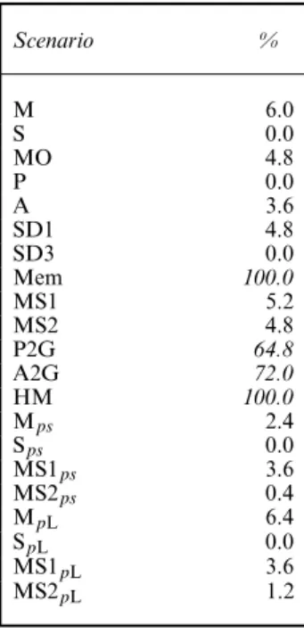
The results of the adapted test are shown in Table 7 for the global test (obtained from summing theχ2-statistics resulting from the adapted tests by state and occasion). The adapted WBWA test is no longer sensitive to a mover–stayer structure (around 5% of significant results), whereas it retains its high power to detect memory (100% of significant results for the scenarios considered). However, it still lacks specificity since it remains sensitive to heterogeneity in preferences (64.8% for P2G; 72% for A2G) and heterogeneity in movement (100% of significant results).

The possible outcomes of the adapted WBWA test and test of positive association are shown in Table 8. Both tests used together facilitate the detection of a mover–stayer structure, and the presence of memory, separately from other phenomena such as heterogeneous groups of preference or movement among the animals. Indeed, if both tests yield significant results, this is indicative of memory. A significant result for the adapted WBWA test alone is indicative of heterogeneity in movement or preferences, whereas a significant result for only the adapted test of positive association is indicative of the existence of a mover–stayer structure.

5. Application to Canada geese

The Canada geese data set from Hestbeck et al. (1991) is very often used as an illustration of memory (see for example Pradel et al. (2005) and Rouan et al. (2009)); it consists of 21435 migrant geese individually marked with neckbands and reobserved at their wintering locations

Table 7. Global test WBWA adapted for memory†

Scenario % M 6.0 S 0.0 MO 4.8 P 0.0 A 3.6 SD1 4.8 SD3 0.0 Mem 100.0 MS1 5.2 MS2 4.8 P2G 64.8 A2G 72.0 HM 100.0 Mps 2.4 Sps 0.0 MS1ps 3.6 MS2ps 0.4 M_pL 6.4 S_pL 0.0 MS1pL 3.6 MS2pL 1.2

†High percentages of significant results (greater than 50%) are in italics.

Table 8. How to interpret combinations of significant test results

Adapted Positive Conclusion

WBWA association test

Yes No Heterogeneity in movement or preferences

Yes Yes Memory

No Yes Mover–stayer structure

each year, between 1984 and 1989 (Hestbeck et al., 1991; Rouan et al., 2009). These wintering sites constituted the states in the capture–recapture experiment: 1 denoted mid-Atlantic (New York, Pennsylvania and New Jersey), 2 Chesapeake (Delaware, Maryland and Virginia) and 3 Carolinas (North and South Carolina). Because we have demonstrated that the existing test WBWA may be indicative of phenomena other than memory affecting transition probabilities, we re-examine the geese data set, using the combination of our new test and adapted WBWA test to determine whether we still reach the same conclusion of memory.

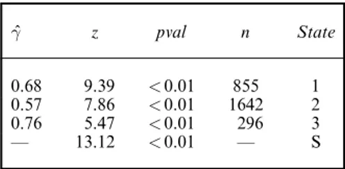
Table 9 shows that the test of positive association yields a significant result.p=0:01/; we have also detailed the test split by state, mainly to show how many animals were used for the test. The adapted WBWA test also yields a significant result.p < 0:001/. According to Table 8, there is significant evidence that the geese display memory, which confirms the previous findings.

Table 9. Canada geese: adapted test of pos-itive association for a mover–stayer structure, by state and summarized†

ˆ γ z pval n State 0.68 9.39 < 0:01 855 1 0.57 7.86 < 0:01 1642 2 0.76 5.47 < 0:01 296 3 — 13.12 < 0:01 — S

† ˆγ denotes the gamma estimate; z and pval re-spectively denote the test statistic andp-value for the adapted test of positive association;n denotes the number of animals used for the test; S in the state column indicates the summarized test.

for both memory and a mover–stayer structure, to check whether, for equivalent parameteri-zation of survival and capture probabilities, the model with memory was selected as a better model than the mover–stayer model. Note that we did not go through an exhaustive model fitting process since we aimed only to compare a memory model and a mover–stayer model fitted to the geese data set. The models were fitted by using the program E-SURGE.

Various models have been proposed to account for memory; we chose to fit the memory model of Hestbeck et al. (1991) as this model considers that the probability of movement towards a site which has not been visited at timet − 1 is not influenced by the particular site visited at t − 1 and thus is biologically more realistic than the alternative models of Pradel (2005) and Rouan et al. (2009) which have transition probabilities which are dependent on site at time t − 1 and t. For the mover–stayer model, we used a mixture model with two groups of animals characterized by different transition structures. Movement between groups is not allowed since animals are assumed to be intrinsically either movers or stayers. It should be noted that a model with two groups of animals that are characterized by different transition matrices is appropriate for a broader spectrum of models than just the mover–stayer model; they can be used for other situations of heterogeneity in movement or preferences. However, fitting a strictly mover– stayer model would require additional constraints that are not necessarily straightforward to implement in pre-existing software such as E-SURGE. Thus it is less likely to be routinely fitted in practice than the more general mixture model. The memory model has by far the lower Akaike information criterion value (ΔAIC = 48:39/, supporting our determination that the transition propensity that is demonstrated by the geese is due to a memory effect.

6. Conclusions and discussion

Within this paper we have presented a new test of positive association which can be used in combination with a modified version of an existing multistate capture–recapture test to diag-nose specific departures from modelling assumptions relating to the transition probability. This combined tool can be used for a capture–recapture experiment with at least three live states and three capture occasions.

The advantage of the new tool is that it provides more specific information, without needing any model fitting, and is very powerful under good conditions of large sample size. An appre-ciable limitation is the requirement for reasonable sample sizes so that there are enough testable

data, particularly for the test of positive association. It is not possible to provide strict guidance on the minimum number of individuals or recommended number of sampling occasions as, if the capture probability is high, smaller numbers of individuals would be required compared with situations of low capture. If the sample sizes are small, the test will just lack the power to detect the underlying phenomena and in this situation it is likely that it would be a struggle to obtain meaningful estimates from the more complex models accounting for transition heterogeneity or memory. Further adaptations to the test to be applicable to small sample sizes, e.g. by using permutation tests, are an active area of research.

Biological behaviours are, by essence, more complex than simulated scenarios involving only a clear-cut phenomenon. For instance, animals could present long-term memory; they could also change their moving behaviour over time; if for example individuals search an area before selecting a breeding colony they would first be movers and then stayers. This period of natal dispersal is often difficult to monitor—see for example Henaux et al. (2007). Therefore it is possible that models which account for both heterogeneity and mover–stayer behaviour could be required but it is unlikely to be able to collect sufficient informative data to be able to detect such complex phenomena.

Model fitting to account for mover–stayer, memory or transition heterogeneity behaviour is non-trivial; therefore the tools that are proposed within this paper make a key contribution preventing overly complicated models from being fitted to data which do not exhibit these behaviours.

References

Arnason, A. N. (1972) Parameter estimates from mark-recapture-recovery experiments on two populations subject to migration and death. Res. Popln Ecol.,13, 97–113.

Arnason, A. N. (1973) The estimation of population size, migration rates, and survival in a stratified population. Res. Popln Ecol.,15, 1–8.

Brown, M. B. and Benedetti, J. K. (1977) Sampling behaviour of tests for correlation in two-way contingency tables. J. Am. Statist. Ass.,72, 309–315.

Brownie, C., Hines, J. E., Nichols, J. D., Pollock, K. H. and Hestbeck, J. B. (1993) Capture-recapture studies for multiple strata including non-Markovian transitions. Biometrics,49, 1173–1187.

Burnham, K. P. (1991) On a unified theory for release-resampling of animal populations. In Proc. 1990 Taipei Symp. Statistics (eds M. T. Chao and P. E. Cheng), pp. 1–35. Taipei: Institute of Statistical Science.

Chabanne, D. B. H., Pollock, K. H., Finn, H. and Bejder, L. (2017) Applying the multistate capture recapture robust design to characterize metapopulation structure. Meth. Ecol. Evoln,8, 1547–1557.

Choquet, R., Lebreton, J.-D., Gimenez, O., Reboulet, A.-M. and Pradel, R. (2009) U-CARE: utilities for per-forming goodness-of-fit tests and manipulating CApture-REcapture data. Ecography,32, 1071–1074. Crespin, L., Harris, M. P., Lebreton, J.-D., Frederiksen, M. and Wanless, S. (2006) Recruitment to a seabird

population depends on environmental factors and on population size. J. Anim. Ecol.,75, 228–238.

Everitt, B. S. (1992) The Analysis of Contingency Tables. London: Chapman and Hall.

Gillingham, M. A. F., Cezilly, F., Wattier, R. and Bechet, A. (2013) Evidence for an association between post-fledging dispersal and microsatellite multilocus heterozygosity in a large population of greater flamingos. PLOS One,8, article e81118.

Gimenez, O., Cam, E. and Gaillard, J.-M. (2018a) Individual heterogeneity and capture-recapture models: what, why and how? Oikos,127, 664–686.

Gimenez, O., Lebreton, J., Choquet, R. and Pradel, R. (2018b) R2Ucare: an R package to perform goodness-of-fit tests for capture-recapture models. Meth. Ecol. Evoln,9, 1749–1754.

Gowan, T. A., Ortega-Ortiz, J., Hostetler, J. A., Hamilton, P. K., Knowlton, A. R., Jackson, K. A., George, R. C., Taylor, C. R. and Naessig, P. J. (2019) Temporal and demographic variation in partial migration of the North Atlantic right whale. Scient. Rep.,9, article 353.

Henaux, V., Bregnballe, T. and Lebreton, J.-D. (2007) Dispersal and recruitment during population growth in a colonial bird, the great cormorant. J. Avn Biol.,38, 44–57.

Hestbeck, J. B., Nichols, J. D. and Malecki, R. A. (1991) Estimates of movement and site fidelity using mark-resight data of wintering Canada geese. Ecology,72, 523–533.

Jeyam, A., McCrea, R. S. and Pradel, R. (2018) A test of positive association for detecting heterogeneity in capture for capture-recapture data. J. Agric. Biol. Environ. Statist.,23, 1–19.

King, R. and Langrock, R. (2016) Semi-Markov Arnason-Schwarz models. Biometrics,72, 619–628.

Lebreton, J.-D., Nichols, J. D., Barker, R. J., Pradel, R. and Spendelow, J. A. (2009) Modeling individual animal histories with multistate capture-recapture models. Adv. Ecol. Res.,41, 87–173.

Lebreton, J.-D. and Pradel, R. (2002) Multistate recapture models: modelling incomplete individual histories. J. Appl. Statist.,29, 353–369.

McCrea, R. S. and Morgan, B. J. T. (2014) Analysis of Capture-recapture Data. Boca Raton: Chapman and Hall. Meyer, D., Zeileis, A. and Hornik, K. (2006) The Strucplot framework: visualizing multi-way contingency tables

with vcd. J. Statist. Softwr.,17, 1–48.

Pradel, R. (2005) Multievent: an extension of multistate capture-recapture models to uncertain states. Biometrics,

61, 442–447.

Pradel, R., Gimenez, O. and Lebreton, J.-D. (2005) Principles and interest of GOF for multistate capture-recapture models. Anim. Biodiv. Conservn,28, 189–204.

Pradel, R., Wintrebert, C. M. A. and Gimenez, O. (2003) A proposal for a goodness-of-fit test to the Arnason-Schwarz multisite capture-recapture model. Biometrics,59, 43–53.

R Core Team (2017) R: a Language and Environment for Statistical Computing. Vienna: R Foundation for Statistical Computing.

Rodrigues, P., Margheri, A., Rebelo, C. and Gomes, M. G. M. (2009) Heterogeneity in susceptibility to infection can explain high reinfection rates. J. Theor. Biol.,259, 280–290.

Roe, J. H., Brinton, A. C. and George, A. (2009) Temporal and spatial variation in landscape connectivity for a freshwater turtle in a temporally dynamic wetland system. Ecol. Appl.,19, 1288–1299.

Rouan, R., Choquet, R. and Pradel, R. (2009) A general framework for modeling memory in capture-recapture data. J. Agric. Biol. Environ. Statist.,14, 338–355.

Schaub, M. and von Hirschheydt, J. (2009) Effect of current reproduction on apparent survival, breeding dispersal, and future reproduction in barn swallows assessed by multistate capture-recapture models. J. Anim. Ecol.,78, 625–635.

Schwarz, C. G., Schweigert, J. F. and Arnason, A. N. (1993) Estimating migration rates using tag-recovery data. Biometrics,59, 291–318.

Shafer, A. B. A., Poissant, J., Cote, S. D. and Coltman, D. W. (2011) Does reduced heterozygosity influence dispersal?: A test using spatially structured populations in an alpine ungulate. Biol. Lett.,7, 433–435. Spilerman, S. (1972) Extensions of the mover-stayer model. Am. J. Sociol.,78, 599–626.

Supporting information

Additional ‘supporting information’ may be found in the on-line version of this article: ‘Web-based supplementary materials for Heterogeneity in transition probabilities’.