HAL Id: hal-02643847
https://hal.inrae.fr/hal-02643847
Submitted on 28 May 2020
HAL is a multi-disciplinary open access
archive for the deposit and dissemination of
sci-entific research documents, whether they are
pub-lished or not. The documents may come from
teaching and research institutions in France or
abroad, or from public or private research centers.
L’archive ouverte pluridisciplinaire HAL, est
destinée au dépôt et à la diffusion de documents
scientifiques de niveau recherche, publiés ou non,
émanant des établissements d’enseignement et de
recherche français ou étrangers, des laboratoires
publics ou privés.
Christoph Rheinberger, Hans E. Romang, Michael Bründl
To cite this version:
Christoph Rheinberger, Hans E. Romang, Michael Bründl. Proportional loss functions for debris
flow events. Natural Hazards and Earth System Sciences, European Geosciences Union, 2013, 13 (8),
pp.2147-2156. �10.5194/nhess-13-2147-2013�. �hal-02643847�
Nat. Hazards Earth Syst. Sci., 13, 1–10, 2013 www.nat-hazards-earth-syst-sci.net/13/1/2013/ doi:10.5194/nhess-13-1-2013
© Author(s) 2013. CC Attribution 3.0 License.
Advances in
Geosciences
Open
Access
Natural Hazards
and Earth System
Sciences
Open AccessAnnales
Geophysicae
OpenAccess
Nonlinear Processes
in Geophysics
Open AccessAtmospheric
Chemistry
and Physics
Open AccessAtmospheric
Chemistry
and Physics
Open Access DiscussionsAtmospheric
Measurement
Techniques
Open AccessAtmospheric
Measurement
Techniques
Open Access DiscussionsBiogeosciences
Open Access Open AccessBiogeosciences
DiscussionsClimate
of the Past
Open Access Open AccessClimate
of the Past
DiscussionsEarth System
Dynamics
Open Access Open AccessEarth System
Dynamics
DiscussionsInstrumentation
Methods and
Data Systems
Open AccessInstrumentation
Methods and
Data Systems
Open Access DiscussionsModel Development
Open Access Open AccessModel Development
DiscussionsHydrology and
Earth System
Sciences
Open AccessHydrology and
Earth System
Sciences
Open Access DiscussionsOcean Science
Open Access Open AccessOcean Science
DiscussionsSolid Earth
Open Access Open AccessSolid Earth
DiscussionsThe Cryosphere
Open Access Open AccessThe Cryosphere
DiscussionsNatural Hazards
and Earth System
Sciences
Open
Access
Discussions
Proportional loss functions for debris flow events
C. M. Rheinberger1, H. E. Romang2, and M. Br ¨undl31LERNA-INRA, Toulouse School of Economics, Toulouse, France
2Swiss Federal Office of Meteorology and Climatology, Zurich, Switzerland 3WSL Institute for Snow and Avalanche Research SLF, Davos, Switzerland Correspondence to: M. Br¨undl ([email protected])
Received: 18 December 2012 – Published in Nat. Hazards Earth Syst. Sci. Discuss.: – Revised: 25 June 2013 – Accepted: 8 July 2013 – Published:
Abstract. Quantitative risk assessments of debris flows and other hydrogeological hazards require the analyst to predict damage potentials. A common way to do so is by use of pro-portional loss functions. In this paper, we analyze a uniquely rich dataset of 132 buildings that were damaged in one of five large debris flow events in Switzerland. Using the double generalized linear model, we estimate proportional loss func-tions that may be used for various prediction purposes includ-ing hazard mappinclud-ing, landscape planninclud-ing, and insurance pric-ing. Unlike earlier analyses, we control for confounding ef-fects of building characteristics, site specifics, and process in-tensities as well as for overdispersion in the data. Our results suggest that process intensity parameters are the most mean-ingful predictors of proportional loss sizes. Cross-validation tests suggest that the mean absolute prediction errors of our models are in the range of 11 %, underpinning the accurate-ness of the approach.
1 Introduction
Landslides are a major hydrogeological hazard in mountain ranges all over the globe. Debris flows are a particularly de-structive form of fast-moving landslides. Over the past 25 yr, debris flows have killed more than 200 people and caused more than C5 billion in economic damages throughout the European Alps (rough estimate based on Guzzetti et al., 2005; Fuchs, 2009; Hilker et al., 2009). In Switzerland alone, debris flows have caused direct economic damages of C340 million, which equals about 5 % of the total amount of losses from hydrological hazards during this period (Hilker et al., 2009).
It is therefore not surprising that considerable effort has been made to understand the physical processes of debris flows (Iverson, 1997; Major and Pierson, 1992; Rickenmann, 1999; Sosio and Crosta, 2009). Less emphasis has been given to damages caused by debris flows. The quantification of po-tential losses is, however, a building block of any quantitative risk assessment (Bonachea et al., 2009; Br¨undl et al., 2009), and serves as the foundation for the planning of mitigation measures (Dai et al., 2002; Romang et al., 2003; Margreth and Romang, 2010).
As the size and force of a debris flow is a priori un-known, quantitative risk assessments are based on predic-tions of damages that could occur under different hazard sce-narios. The term physical vulnerability is commonly used to refer to the proportional loss (also known as relative damage) that an element at risk faces as result of a specific hazard im-pact (Fuchs, 2009; Uzielli et al., 2008; Hollenstein, 2005). This impact is determined by two factors. One is the inten-sity of the hazard, which may be defined as “a set of spatially distributed parameters describing the destructiveness” of the hazard process (Hungr, 1997). The other is the susceptibility of the element at risk, which describes the propensity of a building or other infrastructure to suffer damage from a spe-cific hazard impact (Uzielli et al., 2008).
Empirical analyses that relate damages from debris flows and other landslide processes to intensity and susceptibility factors are still rare; see Totschnig and Fuchs (2013) for a re-cent review of the literature. Most existing studies use either descriptive methods (e.g., Bell and Glade, 2004) or ordinary least-square (OLS) regression (e.g., Fuchs et al., 2007) to ex-plain the proportional loss y= d/v, defined as the ratio of observed damage d to total value v.
While of practical value, there are some drawbacks with these conventional approaches. The descriptive approach does not make full use of the available information and al-lows only for qualitative damage predictions. OLS regression can incorporate intensity and susceptibility factors, but its ap-plicability is limited by the fact that regression estimates are unconstrained, allowing for loss estimates to take on implau-sibly large or small values.
Since the proportional loss is by construction a relative measure, valid models must provide estimates of y restricted to the [0, 1] interval. One can constrain OLS to this range, but the resulting censored linear model bears some unattractive features (Kieschnick and McCullough, 2003; Fox, 2008). It is inherently unstable because it critically depends on the values at which minimal and maximal loss is predicted, it is inexpedient as soon as more than one predictor variable is included, the abrupt truncation of the linear slope of y is unrealistic as one would expect a smooth rather than a kinked relationship between the proportional loss and the predictor variables, and its error variance is most likely not constant (i.e., heteroscedastic) because regressions involving data from the unit interval typically display more variation around the mean than at the limits of the [0, 1] interval.
Generalized linear models (GLMs) provide a natural framework for the estimation of proportional data (De Jong and Heller, 2008). Geoscientists have previously made use of this property to predict the occurrence probability of de-bris flow events (Ohlmacher and Davis, 2003; Sepulveda and Padilla, 2008; Griffiths et al., 2004). Yet apart from recent studies by Totschnig et al. (2011) and Totschnig and Fuchs (2013), GLMs have to the best of our knowledge not been used to analyze proportional loss data of debris flow events.
Moreover, there is a caveat to the application of standard GLMs such as logistic or probit regression to proportional loss data. GLMs typically assume that the error variance is constant across observations. This assumption is likely to be violated whenever damages are spatially or temporally cor-related. Ignoring the non-constant nature of the error vari-ances may result in a misrepresentation of the true dispersion and erroneous inferences about the parameters of interest (De Jong and Heller, 2008).
In this paper we use the double generalized linear model (DGLM) introduced by Smyth (1989) to explore a unique dataset comprising insurance values of 132 buildings. These buildings were damaged by five debris flow events, which oc-curred in Switzerland during the late 1980s and early 2000s. While the DGLM provides the same flexibility as standard GLMs, it adjusts for the overdispersion typically observed in proportional losses, and hence lends itself for the statistical analysis of our dataset.
The remainder of the paper is structured as follows. Sec-tion 2 describes our empirical strategy, our dataset, and the statistical approach in more detail. Section 3 presents re-gression results and sensitivity tests that assess the predic-tion accuracy of the estimated proporpredic-tional loss funcpredic-tions.
In Sect. 4, we sum up with some remarks on the usefulness of our approach for the practical management of debris flow hazards.
2 Data and methods 2.1 Conceptual framework
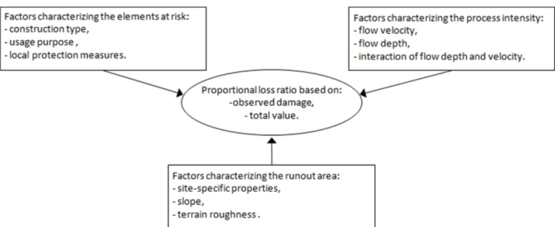
The conceptual framework of our empirical analysis of phys-ical vulnerability toward debris flow events is illustrated in Fig. 1. Based on Dai et al. (2002), we identified three build-ing blocks for the statistical analysis of debris flow risk: (1) the runout area, (2) the process intensity, and (3) the elements at risk. In the empirical analysis, we seek to explain observed proportional losses by predictor variables characterizing the three building blocks.
In the empirical analysis, we define the runout area by its roughness and its slope steepness. We characterize the pro-cess intensity by the impact angle between the tangent to the flow path of the debris flow at the point of impact and the plane tangent to the struck surface at the point of im-pact, the flow depth and velocity, and their interaction, which is widely accepted as an intensity indicator (Kreibich et al., 2009). Flow depth and velocity are used not only as crite-ria for distinguishing intensity zones for hazard mapping of debris flows (Loat and Petrascheck, 1997) but also in risk analyses in Switzerland (Br¨undl et al., 2009), which was the main argument for preferring them to other approaches such as, e.g., the velocity head used only for comparison reasons in this paper (see Sect. 2.2). Elements at risk are described by their type (concrete, lightweight, or mixed construction), purpose (agricultural, industrial, or residential use), and the presence or absence of object-specific protection measures such as reinforced walls or sheet pilings. Below, the data col-lection process is described in more detail.
2.2 Data
We focused on five major debris flow events that had oc-curred in the Swiss Alps during the late 1980s and early 2000s. According to the size classification by Jakob (2005) these events all belonged to class 4 debris flows with to-tal volumes ranging from 10 000 to 75 000 m3. They caused damages with a total amount of C25 million on 455 build-ings corresponding to average damages of roughly C50 000 per affected building. Of these 455 buildings, 132 were even-tually selected for analysis. Data selection was based on the availability of sufficiently accurate documentation of the runout area, the process intensity, and the elements at risk (in-cluding their total values and the observed damages). Dam-age observations were split approximately evenly across haz-ard sites. Figure 2 details out the geographical distribution of the debris flow events and the analyzed damages.
In recent years debris flows in Switzerland have been reg-istered in a central database (Hilker et al., 2009). However,
Please note the remarks at the end of the manu script.
Fig. 1. Conceptual framework for the empirical analysis of proportional loss data.
Fig. 2. Summary of the analyzed hazard sites including information about the location, date, total debris volume, and number of affected and of analyzed buildings.©Federal Office of Topography swisstopo.
the event descriptions in this database are insufficient for object-specific statistical analyses. Therefore, we had to im-prove the data quality (see Romang, 2004; Kimmerle, 2002). We assessed type and purpose of each of the buildings based on field observations and interviews with affected property owners and other witnesses of the debris flow events. Ab-solute and relative damages were ascertained based on in-surance reports of actuarial building values and the costs of repair or replacement. The process intensity of the analyzed debris flow events was reconstructed from back modelingCE1 with FLO-2D (O’Brien et al., 1993) and back calculations of
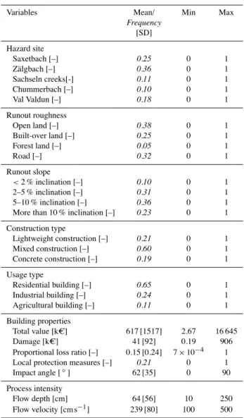
the flow velocity, flow depth, and impact pressures (Hungr et al., 1984). Information about the runout topography, rough-ness, and inclination was collected directly in the field. Ta-ble 1 gives a descriptive summary of the compiled dataset.
Data quality is accurate for all parameters that could be di-rectly observed or measured. The intensity parameters could, however, not be measured directly and their quantification is therefore fraught with some uncertainty. We reduced this un-certainty by combining back calculations, engineering rules of thumb, and eyewitness reports (Romang, 2004). In partic-ular, we could reconstruct in many cases the maximum
depo-Please note the remarks at the end of the manu script.
Table 1. Descriptive statistics of the compiled dataset (N= 132).
Variables Mean/ Min Max
Frequency [SD] Hazard site Saxetbach [–] 0.25 0 1 Z¨algbach [–] 0.36 0 1 Sachseln creeks[-] 0.11 0 1 Chummerbach [–] 0.10 0 1 Val Valdun [–] 0.18 0 1 Runout roughness Open land [–] 0.38 0 1 Built-over land [–] 0.25 0 1 Forest land [–] 0.05 0 1 Road [–] 0.32 0 1 Runout slope <2 % inclination [–] 0.10 0 1 2–5 % inclination [–] 0.31 0 1 5–10 % inclination [–] 0.36 0 1
More than 10 % inclination [–] 0.23 0 1 Construction type Lightweight construction [–] 0.21 0 1 Mixed construction [–] 0.60 0 1 Concrete construction [–] 0.19 0 1 Usage type Residential building [–] 0.65 0 1 Industrial building [–] 0.24 0 1 Agricultural building [–] 0.11 0 1 Building properties Total value [k C] 617 [1517] 2.67 16 645 Damage [k C] 41 [92] 0.19 906
Proportional loss ratio [–] 0.15 [0.24] 7⇥ 10 4 1 Local protection measures [–] 0.21 0 1
Impact angle [ ] 62 [35] 0 90
Process intensity
Flow depth [cm] 64 [56] 10 250
Flow velocity [cm s 1] 239 [80] 100 500 SD is the standard deviation.
sition height (Hmax D)based on marks left on exterior walls. According to the Bernoulli principle, Hmax D equals the ve-locity head V2/(2· g) (with g = 9.81 ms 2TS1). By solving the equation for V=p2· g · Hmax Dwe obtained an estimate of the flow velocity, which we then compared to the flow velocity estimated based on the procedure described in Egli (2005). If the discrepancy between both estimates was larger than 1 m s 1, we reassessed the flow velocity.
The outlined data validation process significantly im-proved the data quality. Yet we emphasize that in the af-termath of an event a clear distinction between debris flows and hyper-concentrated flows is not always possible because different hazard processes may coincide. For example, the runout area might first be hit by a debris flow surge and subsequently flooded and eroded again (Pierson, 2005). We are unable to differentiate between such transitional forms of flowing and flooding processes. For the purpose of our
anal-ysis, this limitation seems acceptable. Totschnig and Fuchs (2013) provide further support for this assumption.
2.3 Statistical approach
The statistical modeling of proportional loss functions in the standard GLM framework is based upon three components (Fox, 2008): (1) the loss function, ⌘i= Xi⇥ , where XiTS2 is a linear combination of predictor variables for object i, and is the corresponding vector of coefficients; (2) a prob-ability distribution of proportional loss from the exponential family; and (3) an invertible link function g that maps the expected proportional loss E[yi] = µionto the predictors so that g(µi)= ⌘i.
Specific link functions have emerged for the analysis of proportional loss data (De Jong and Heller, 2008). The canonical link is the logit
⌘i= log(di/(vi, di))= log(yi/(1 yi)) ,
where vi and di denote the total value of and the damage to object i both measured in units of k C. Since the log odds ratio approaches negative infinity as yi approaches 0, and moves toward positive infinity as yi approaches 1, loss pre-dictions are restricted to the [0, 1] interval.
The logit link gives rise to the standard logistic regression model
yi = (1 + exp( ⌘i)) 1,
which can be evaluated by maximum likelihood methods. Applied to polytomous data, the model assumes that the proportional loss yi observed at object i is binomially dis-tributed: yi⇠ B(vi, di)8i 2 N, where N is the set of all ob-servations. This implies that each object at risk can be di-vided into ni= vi/kCequal units, which the model treats as if they were independent Bernoulli trials with probability pi= di/vi.
This distributional assumption becomes unrealistic when the damage potential is spatially or temporally correlated. A simple example is a debris flow hitting a residential building of total value vi, but only the ground floor is affected. Now, assume that the first floor bears less (or more) valuables than the ground floor. In this case, the dispersion across the ob-served units of proportional loss is larger than warranted by the constant error variance assumption of the logistic regres-sion model: Var[yi] = yi(1 yi), where is a dispersion parameter common to all observations.
The DGLM generalizes the above error variance by in-clusion of an observation-specific dispersion parameter i, which is contingent on some predictor variables to account for systematic variations in the error variance (Smyth, 1989). The observation-specific dispersion parameter can be ex-pressed as h( i)= Zi⇥ , where Ziis a vector of predictors and is the corresponding coefficient vector. (Note that Zi can be a perfect subset of Xi. Identification is warranted as long as comprises a freely estimable intercept.)
Please note the remarks at the end of the manu script.
The joint estimation of the dispersion submodel h( i)and the loss submodel g(µi)increases the precision in the coef-ficient estimates of interest because observations with larger variation are penalized (i.e., they are down-weighted in the likelihood maximization). Standard errors for the predictors of both the loss and the dispersion submodels are calculated from the inverse Fisher-information matrix and Wald tests can be used to infer the significance level of a specific pre-dictor (Smyth, 1989). The interpretation of the coefficient es-timates from the DGLM with logit link is therefore identical to the interpretation of those obtained from a standard logis-tic regression model.
A virtue of this class of models is the ease with which co-efficient estimates can be converted to and interpreted as risk ratios (De Jong and Heller, 2008). Risk ratios are particularly insightful to compare the vulnerability of different types of buildings. In general terms, the risk ratio is defined as RR[x0]=E ⇥ y|x0= 1, ¯X0⇤ E⇥y|x0= 0, ¯X0⇤ = 1+ exp ¯X0 1+ exp ¯X0 + 0 x , (1)
where x0 is the coefficient on the characteristic of interest x0. E⇥y| ¯X0, x0= 1⇤ and E⇥y| ¯X0, x0= 0⇤ denote the expected proportional loss for buildings that do (x0= 1) and do not have (x0= 0) this characteristic, keeping all other predictors
¯X0fixed at sample means.
A common assumption is that the log-transformed risk ratio is normally distributed: log RR[x0] ⇠ N µ, 2 . The mean is equal to the log of the expected risk ra-tio: µ= log E⇥y|x0= 1, ¯X0⇤/E⇥y|x0= 0, ¯X0⇤ . Using the delta method (Fox, 2008), the variance can be approximated by 2⇡Var ⇥ y|x0= 1, ¯X0⇤ E⇥y|x0= 1, ¯X0⇤2 + Var⇥y|x0= 0, ¯X0⇤ E⇥y|x0= 0, ¯X0⇤2 2· Cov ⇥ y|x0= 1, ¯X0;y|x0= 0, ¯X0⇤ E⇥y|x0= 1, ¯X0⇤E⇥y|x0= 0, ¯X0⇤ , (2) where Var[.] and Cov[.] denote the sample variance and covariance. (A detailed derivation of Eq. 2 is given in Appendix A1.) Based on this, the 95 % confidence inter-val (95 % CI) around the risk ratio is calculated as CI= exp [µ± 1.96 · ].
3 Results
3.1 Regression models
We present coefficient estimates for three specifications of the DGLM with logit link function. These specifications dif-fer with respect to the predictor variables included in the loss and dispersion functions.
3.1.1 Model ITS3
The first model specification explains observed proportional losses solely through intensity predictors. The dispersion function includes a global constant and site-specific con-stants that control for differences in dispersion across de-bris flow sites. The loss function includes the impact angle (A), flow depth (D), flow velocity (V ), and their interaction (D· V ), which we take as an intensity indicator. We use log transformations to reduce skew in the distribution of these predictors. Note that log D· logV is a non-linear transforma-tion of log D· V2, which others have proposed as a surrogate measure of impact force (Jakob et al., 2012; Kreibich et al., 2009).
Regression results reported in Table 2 indicate that the expected loss is significantly determined by the four in-tensity predictors. The coefficient on the logged impact angle is positive, but the effect of a larger impact an-gle on the loss function is negligibly small. To see this, consider two impact angles A1 and A2= 2 · A1. Since the predictor is log-transformed, the effect of doubling the impact angle while keeping everything else constant is 0.224· (logA2 log A1)= 0.224 · logA2/A1⇡ 0.155. In other words, the loss function increases by only 0.155 units for every doubling of the impact angle.
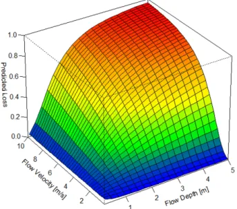
Coefficients on the flow depth and velocity are both neg-ative, but the coefficient on the interaction term is posi-tive. This implies that proportional losses grow with in-creasing flow depth (@y/@D > 0) and velocity (@y/@V > 0), but the growth rate is marginally decreasing (@2y/@D2<0, @2y/@V2<0). In Fig. 3, we visualize this relationship by plotting the proportional losses predicted from Model I for debris flow depths and velocities typically assumed in the design of local protection strategies (Egli, 2005). The reader is warranted that D and V are positively correlated (Pear-son’s rho= 0.26, P < 0.01), so that combinations with low (high) velocities and large (small) depths are unlikely to be observed in reality. Therefore, the interpretation of model predictions for such out-of-bounds combinations is meaning-less.
The significant intercept of the dispersion function un-derlines that there is overdispersion in our data. Moreover, the dispersion varies across hazard sites and is significantly lower for the Chummerbach event, suggesting more homoge-nous damages at this hazard site.
3.1.2 Model II
The second model specification adds site-specific and object-specific attributes to the loss function. A likelihood-ratio test confirms that the model fit is significantly improved by the inclusion of the additional predictors ( 9df2 : 15.8, P < 0.05). No differences are observed across the five hazard sites. With the exception of the insignificant coefficient on the impact angle, coefficient estimates on the intensity predictors are
Please note the remarks at the end of the manu script.
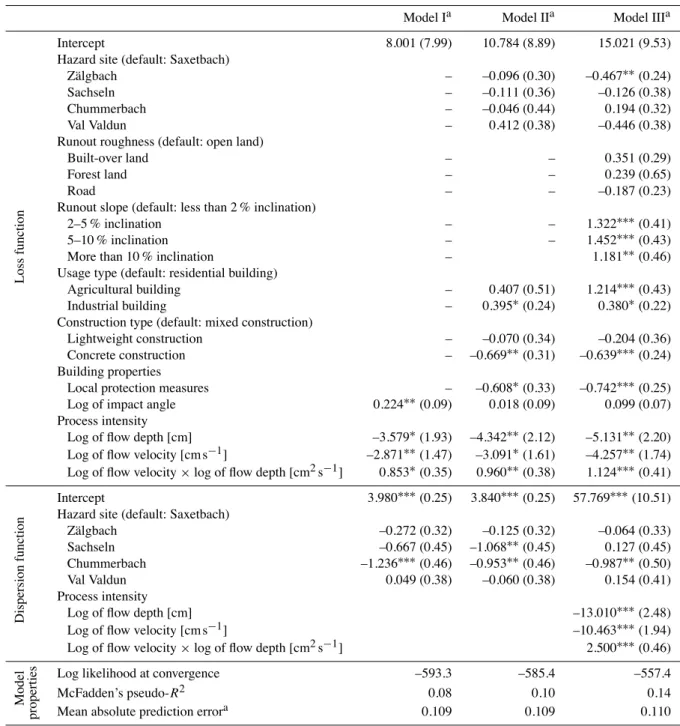
Table 2. Regression results of different DGLM specifications; standard errors are reported in brackets.
Model Ia Model IIa Model IIIa
Loss
function
Intercept 8.001 (7.99) 10.784 (8.89) 15.021 (9.53)
Hazard site (default: Saxetbach)
Z¨algbach – –0.096 (0.30) –0.467⇤⇤(0.24)
Sachseln – –0.111 (0.36) –0.126 (0.38)
Chummerbach – –0.046 (0.44) 0.194 (0.32)
Val Valdun – 0.412 (0.38) –0.446 (0.38)
Runout roughness (default: open land)
Built-over land – – 0.351 (0.29)
Forest land – – 0.239 (0.65)
Road – – –0.187 (0.23)
Runout slope (default: less than 2 % inclination)
2–5 % inclination – – 1.322⇤⇤⇤(0.41)
5–10 % inclination – – 1.452⇤⇤⇤(0.43)
More than 10 % inclination – 1.181⇤⇤(0.46)
Usage type (default: residential building)
Agricultural building – 0.407 (0.51) 1.214⇤⇤⇤(0.43)
Industrial building – 0.395⇤(0.24) 0.380⇤(0.22)
Construction type (default: mixed construction)
Lightweight construction – –0.070 (0.34) –0.204 (0.36)
Concrete construction – –0.669⇤⇤(0.31) –0.639⇤⇤⇤(0.24)
Building properties
Local protection measures – –0.608⇤(0.33) –0.742⇤⇤⇤(0.25)
Log of impact angle 0.224⇤⇤(0.09) 0.018 (0.09) 0.099 (0.07)
Process intensity
Log of flow depth [cm] –3.579⇤(1.93) –4.342⇤⇤(2.12) –5.131⇤⇤(2.20) Log of flow velocity [cm s 1] –2.871⇤⇤(1.47) –3.091⇤(1.61) –4.257⇤⇤(1.74) Log of flow velocity⇥ log of flow depth [cm2s 1] 0.853⇤(0.35) 0.960⇤⇤(0.38) 1.124⇤⇤⇤(0.41)
Dispersion
function
Intercept 3.980⇤⇤⇤(0.25) 3.840⇤⇤⇤(0.25) 57.769⇤⇤⇤(10.51)
Hazard site (default: Saxetbach)
Z¨algbach –0.272 (0.32) –0.125 (0.32) –0.064 (0.33)
Sachseln –0.667 (0.45) –1.068⇤⇤(0.45) 0.127 (0.45)
Chummerbach –1.236⇤⇤⇤(0.46) –0.953⇤⇤(0.46) –0.987⇤⇤(0.50)
Val Valdun 0.049 (0.38) –0.060 (0.38) 0.154 (0.41)
Process intensity
Log of flow depth [cm] –13.010⇤⇤⇤(2.48)
Log of flow velocity [cm s 1] –10.463⇤⇤⇤(1.94)
Log of flow velocity⇥ log of flow depth [cm2s 1] 2.500⇤⇤⇤(0.46)
Model
properties
Log likelihood at convergence –593.3 –585.4 –557.4
McFadden’s pseudo-R2 0.08 0.10 0.14
Mean absolute prediction errora 0.109 0.109 0.110
aSignificance coding for Wald tests on coefficient estimates:⇤⇤⇤<0.01,⇤⇤<0.05,⇤<0.1;bsee the description in Sect. 3.2.
similar to those obtained with Model I. This suggests site-specific factors in Model II do not have a strong confound-ing relationship with the process intensity but help to explain variability in the data.
Coefficient estimates on object-specific characteristics im-ply that proportional losses at industrial buildings are signif-icantly larger than those observed for residential buildings, while proportional losses at agricultural buildings are statis-tically not different from those observed for residential build-ings. Concrete buildings are significantly less vulnerable to
debris flow damages, as are buildings that had local protec-tion measures installed.
With Eq. (1) we can study how much the construction type, the usage purpose, or the implementation of local protec-tion measures reduces or increases the expected proporprotec-tional loss. As an illustrative example, consider two buildings of the same type and value but one is protected by sheet pilings, while the other is not. The risk ratio is RR⇥x0= protection⇤= 0.62(CI: 0.42,0.89), meaning that we expect a ⇠ 38 %
Fig. 3. Proportional loss predictions by Model I for commonly ob-served debris flow depths and velocities (2008: 411). To construct this plot, the impact angle was fixed at the sample means of 64 .
smaller loss at the protected building. Similar risk ratios for other predictors of interest are reported in Table 3.
3.1.3 Model III
This specification includes all available information in the loss function. Additionally, we amend the dispersion func-tion with predictors of the flow height, flow velocity, and their interaction. In terms of statistical fit, the improvement over Model II is significant ( 2
10df: 55.9, P < 0.001). This improvement is largely due to the improved capture of het-erogeneity in the dispersion function. Inclusion of the inten-sity predictors into the dispersion function accounts for vari-ation in dispersion at the building level rather than the hazard site level.
The site-specific constants indicate that losses observed at the Z¨algbach site are significantly smaller than those ob-served at the other hazard sites. Once we control for event-specific factors, the other sites are statistically not different from each other. Information about the runout cover is not predictive. However, proportional losses increase with runout steepness.
Results of Model III support the finding that industrial buildings are more vulnerable to debris flow damages than residential buildings. Controlling for additional dispersion in the data, we now also find a significant effect on agricultural buildings. Concrete buildings and buildings where local pro-tection measures were installed are significantly less vulner-able to debris flows than mixed or light constructions (Ta-ble 3). Coefficient estimates on the intensity predictors are again similar to those obtained with Models I and II, con-firming that they are the most important loss predictors.
Fig. 4. Kernel density plot (Gaussian kernel, bandwidth: 1) of ob-served versus predicted proportional losses for the 132 damaged buildings.
3.2 Prediction accuracy
We use leave-one-out cross validation (LOOCV) to assess the out-of-sample prediction accuracy of our models (Wilks, 2006). This resampling procedure repeatedly fits the DGLM using N 1 observations as training set to make a prediction for the left-out observation. Then, the predicted loss for this observation is compared to the observed loss and prediction accuracy is measured in terms of the mean absolute predic-tion error across every observapredic-tion.
The mean absolute prediction errors for Models I–III are 0.108, 0.109, and 0.110, respectively (Table 2). This suggests that loss predictions based on the three models are on average within a range of±11 % around the observed loss size and that none of the models outperforms the others in terms of prediction quality. This is, however, not to be confused with the statistical fit, which measures at the explanatory power of the included predictors.
To see whether there are ranges within the [0, 1] interval where the predictions are particularly inaccurate, we used Models I–III to predict the proportional losses on the full dataset, and compared predicted losses with observed losses. Figure 4 illustrates that all three models do a decent job of predicting small to medium losses. However, the models do not predict large losses or even total losses. We conclude that while our approach is useful to predict damages of common sizes, it is less suited to predict extreme damages. By defini-tion, these are rare events and we miss sufficient observations in the extreme range of damages that would allow for us to better calibrate the model.
4 Conclusions
The assessment of potential damages is a key ingredient of any risk assessment study. As risk-based decisions play an ever more important role in natural hazard management www.nat-hazards-earth-syst-sci.net/13/1/2013/ Nat. Hazards Earth Syst. Sci., 13, 1–10, 2013
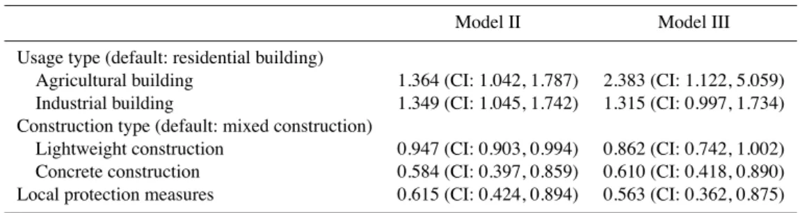
Table 3. Risk ratios for factors characterizing the elements at risk; 95 % confidence intervals are reported in brackets.
Model II Model III
Usage type (default: residential building)
Agricultural building 1.364 (CI: 1.042, 1.787) 2.383 (CI: 1.122, 5.059) Industrial building 1.349 (CI: 1.045, 1.742) 1.315 (CI: 0.997, 1.734) Construction type (default: mixed construction)
Lightweight construction 0.947 (CI: 0.903, 0.994) 0.862 (CI: 0.742, 1.002) Concrete construction 0.584 (CI: 0.397, 0.859) 0.610 (CI: 0.418, 0.890) Local protection measures 0.615 (CI: 0.424, 0.894) 0.563 (CI: 0.362, 0.875) CI is the confidence interval.
(Br¨undl et al., 2009), there has been growing interest in the development of predictive loss functions that could be used to quantify damage potentials for various natural hazards.
In this paper, we have outlined a framework to esti-mate proportional loss functions for debris flow events. The framework lends itself to the analysis of other hydrological hazards. Unlike standard regression models, the presented DGLM can deal with problems of overdispersion, and is therefore a valuable tool for empirical analyses of natural hazard damages.
We have used the DGLM to analyze what is maybe the richest dataset on debris flow damages to date in Switzerland. We find that flow depth, flow velocity, and their interaction are the most meaningful predictors of relative damage. Indus-trial and agricultural buildings tend to be more vulnerable to debris flows than residential buildings. This is most likely due to different value concentrations of the ground floor. Many agricultural and industrial buildings are single-story buildings, which by nature have an increased damage poten-tial within the reach of debris flow surges. Residenpoten-tial build-ings, in contrast, often have their values distributed over sev-eral stories so that the damage potential in the ground floor is relatively small compared to the total damage potential. This underlines the importance of controlling for overdispersion at the building level.
We find some insightful results with regard to building characteristics. These are of particular interest because prop-erty owners can alter them through self-protection efforts. Using the risk ratios reported in Table 3, the damage to a building without local protection measures such as sheet pilings or concrete enforcements is predicted to be 1.6–1.8 times as high as the damage to an otherwise identical non-protected building. Similarly, the damage predicted to a con-crete building is only about 60 % of the damage expected to an otherwise identical non-concrete building, suggesting that structural adaptation to the local environment is an ef-fective means to reduce debris flow damages (Margreth and Romang, 2010).
How accurate are the results? As a LOOCV analysis has confirmed, proportional loss predictions generated with the DGLM approach are quite precise, with mean absolute pre-diction errors in the range of 11 %. From a practical point
of view, this prediction quality is more than sufficient as the uncertainty introduced by the loss predictions is far smaller than that of other parameters entering the risk assessment for debris flow (Schaub and Br¨undl, 2010).
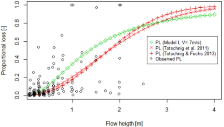
How do the results compare to the proportional loss func-tions found in recent studies by Totschnig et al. (2011) and Totschnig and Fuchs (2013)? We did some rough calcula-tions comparing the proportional loss function obtained from our Model I with the best-fitting loss functions reported in Eq. (7) of Totschnig et al. (2011) and Eq. (3) of Totschnig and Fuchs (2013), respectively. If we keep flow velocity and impact angle fixed at sample means, we obtain loss predic-tions that are about 50 % lower than those of Totschnig et al. (2011); if we assume a flow velocity of 7 m s 1 (the upper range of the values Egli (2005) proposed for debris flows in flat terrain), loss predictions obtained from both models are within a range of 10 % (see Appendix A2 for a visualization). We conclude that, under reasonable assumptions, our loss predictions are in close agreement with those of Totschnig et al. (2011) and Totschnig and Fuchs (2013).
What is the practical value of the results? We may think of several ways to make use of proportional loss predictions by our approach. Here are but two examples. First, modern GIS techniques allow for combining proportional loss functions with hazard maps and databases of insurance contracts to cre-ate proper risk maps. Such risk maps could help hazard man-agers to identify at risk areas and to prioritize among mitiga-tion needs based on the actual damage potential. Second, pri-vate property insurers could use the loss predictions to offer individualized contracts that better reflect each homeowner’s risk. This would lead to a reduction in the overall volume of premiums paid by insurance holders because fair pricing re-duces “moral hazard” – the tendency of the most-exposed in-surance holders not to take self-protection measures, as there are no incentives to do so (Raschky and Weck-Hannemann, 2007). State building insurers (in 19 cantons of Switzerland) could use our results to get an overview as to where house owners should consider building local protection measures.
In conclusion, we believe that the presented approach bears great potential for the prediction of natural hazard dam-ages. Needless to say that, with more data, we will be able to better calibrate the proportional loss functions and to im-Nat. Hazards Earth Syst. Sci., 13, 1–10, 2013 www.nat-hazards-earth-syst-sci.net/13/1/2013/
prove their prediction accuracy. It is therefore of great im-portance to build up and maintain central damage databases – a very good example is the HOWAS 21 database for flood losses (Thieken et al., 2009) – that allow for storing of event-specific information. Our analysis emphasizes that flow depths and heights, observed damages, and total values of damaged buildings are of particular interest.
Appendix A
A1 Derivation of Eq. (2) by the delta method
The variance of the log-transformed risk ratio is a non-linear function, and hence has to be approximated. A common method to do so is the delta method; see, e.g., Fox (2008). Before we derive the variance of log RR[x0] , we introduce a more compact notation. Define
¯yj⌘ E ⇥
y|x0= j, ¯X0⇤ with j= {0,1}, yij⌘ yi|x0= j, ¯X0 8 i 2 N and j = {0,1}, and
f ⌘ log ¯y1/¯y0= log ¯y1 log¯y0.
By the delta method, the variance of the non-linear function f can be approximated as
Var⇥log RR(x0)⇤= rf 6 rfT, whererf denotes the gradient vector rf = @f @¯y1 @f @¯y0 = 1 ¯y1 1 ¯y0 ,
and 6 denotes the variance–covariance matrix 6= N 1
" PN
i=1(yi1 ¯y1)2 PiN=1(yi0 ¯y0) (yi1 ¯y1) PN
i=1(yi1 ¯y1) (yi0 ¯y0) PNi=1(yi0 ¯y0)2 # . By inserting, we have rf 6 rfT = 1 ¯y1 1 ¯y0 · N 1 PN i=1(yi1 ¯y1)2 PN i=1(yi0 ¯y0) (yi1 ¯y1) PN i=1(yi1 ¯y1) (yi0 ¯y0) PN i=1(yi0 ¯y0)2 " 1 ¯y1 1 ¯y0 # = N 1 " PN i=1(yi1 ¯y1)2 ¯y2 1 + PN i=1(yi0 ¯y0)2 ¯y2 0 2 PN i=1(yi1 ¯y1) (yi0 ¯y0) ¯y1¯y0 # = Var [yi1] ¯y2 1 +Var [yi0] ¯y2 0 2Cov [yi1, yi0] ¯y1¯y0 ,
which is equivalent to Eq. (2) in the main text.
Fig. A2.TS5. PL is the proportional loss. CE2
A2 Visual comparison with other proportional loss functions
Comparison of the proportional loss (PL) function of Model I (evaluated at V = 7 ms 1) with the best-fitting PL functions of Totschnig et al. (2011: Eq. 7) and Totschnig and Fuchs (2013, Eq. 3)TS4.
Acknowledgements. This paper was partly funded through EU
FP6 STREP contract no. 081412 (“IRASMOS”). We thank Roland Kimmerle for providing his dataset. We are grateful to Sven Fuchs and three other reviewers, whose comments greatly helped in improving the paper.
Edited by: O. Katz
Reviewed by: S. Fuchs and three anonymous referees
References
Bell, R. and Glade, T.: Quantitative risk analysis for landslides – Ex-amples from B´ıldudalur, NW-Iceland, Nat. Hazards Earth Syst. Sci., 4, 117–131, doi:10.5194/nhess-4-117-2004, 2004. Bonachea, J., Remondo, J., De Ter´an, J. R. D.,
Gonz´alez-D´ıez, A., and Cendrero, A.: Landslide Risk Models for Deci-sion Making, Risk Anal., 29, 1629–1643, doi:10.1111/j.1539-6924.2009.01283.x, 2009.
Br¨undl, M., Romang, H. E., Bischof, N., and Rheinberger, C. M.: The risk concept and its application in natural hazard risk man-agement in Switzerland, Nat. Hazards Earth Syst. Sci., 9, 801– 813, doi:10.5194/nhess-9-801-2009, 2009.
Dai, F. C., Lee, C. F., and Ngai, Y. Y.: Landslide risk assess-ment and manageassess-ment: an overview, Eng. Geol., 64, 65–87, doi:10.1016/S0013-7952(01)00093-X, 2002.
De Jong, P. and Heller, G. Z.: Generalized Linear Models for Insur-ance Data, International Series on Actuarial Science, Cambridge University Press, Cambridge, 2008.
Egli, T.: Wegleitung Objektschutz gegen gravitative Naturgefahren, Vereinigung Kantonaler Feuerversicherer, Bern, Switzerland,
Please note the remarks at the end of the manu script.
available at: http://www.vkf.ch/VKF/Downloads.aspx, last ac-cess:TS6, 2005 (in German).
Fox, J.: Applied Regression Analysis and Generalized Linear Mod-els, 2 Edn., Sage, Thousand Oaks, CA, 2008.
Fuchs, S.: Susceptibility versus resilience to mountain hazards in Austria – paradigms of vulnerability revisited, Nat. Hazards Earth Syst. Sci., 9, 337–352, doi:10.5194/nhess-9-337-2009, 2009.
Fuchs, S., Heiss, K., and H¨ubl, J.: Towards an empirical vulner-ability function for use in debris flow risk assessment, Nat. Hazards Earth Syst. Sci., 7, 495–506, doi:10.5194/nhess-7-495-2007, 2007.
Griffiths, P. G., Webb, R. H., and Melis, T. S.: Frequency and initia-tion of debris flows in Grand Canyon, Arizona, J. Geophys. Res., 109, F04002, doi:10.1029/2003JF000077, 2004.
Guzzetti, F., Stark, C. P., and Salvati, P.: Evaluation of flood and landslide risk to the population of Italy, Environ. Manage., 36, 15–36, doi:10.1007/s00267-003-0257-1, 2005.
Hilker, N., Badoux, A., and Hegg, C.: The Swiss flood and landslide damage database 1972–2007, Nat. Hazards Earth Syst. Sci., 9, 913–925, doi:10.5194/nhess-9-913-2009, 2009.
Hollenstein, K.: Reconsidering the risk assessment concept: Stan-dardizing the impact description as a building block for vulner-ability assessment, Nat. Hazards Earth Syst. Sci., 5, 301–307, doi:10.5194/nhess-5-301-2005, 2005.
Hungr, O.: Some methods of landslide intensity mapping, in: Land-slide Risk Assessment, edited by: Cruden, D. and Fell, R., Balkema, Rotterdam, 1997.
Hungr, O., Morgan, G., and Kellerhals, C.: Quantitative analysis of debris flow torrent hazards for design of remedial measures, Can. Geotech. J., 21, 663–677, doi:10.1139/t84-073, 1984.
Iverson, R. M.: The physics of debris flows, Rev. Geophys., 35, 245–296, doi:10.1029/97RG00426, 1997.
Jakob, M.: A size classification for debris flows, Eng. Geol., 79, 151–161, doi:10.1016/j.enggeo.2005.01.006, 2005.
Jakob, M., Stein, D., and Ulmi, M.: Vulnerability of build-ings to debris flow impact, Nat. Hazards, 60, 241–261, doi:10.1007/s11069-011-0007-2, 2012.
Kieschnick, R. and McCullough, B. D.: Regression analysis of vari-ates observed on (0,1): percentages, proportions and fractions, Stat. Model., 3, 193–213, doi:10.1191/1471082X03st053oa, 2003.
Kimmerle, R.: Schadenempfindlichkeit von Geb¨auden gegen¨uber Wildbachgefahren, Master thesis, University of Bern, Switzer-land, 2002 (in German).
Kreibich, H., Piroth, K., Seifert, I., Maiwald, H., Kunert, U., Schwarz, J., Merz, B., and Thieken, A. H.: Is flow velocity a significant parameter in flood damage modelling?, Nat. Hazards Earth Syst. Sci., 9, 1679–1692, doi:10.5194/nhess-9-1679-2009, 2009.
Loat, R. and Petrascheck, A.: Consideration of Flood Hazards for Activities with Spatial Impact – Recommendations, Federal Of-fice for Water Management (BWW), Federal OfOf-fice for Spatial Planning (BRP), Federal Office for the Environment, Forests and Landscape (BUWAL), Bern, available at: www.bafu.admin.ch, last access: 25 June 2013, 1997.
Major, J. J. and Pierson, T. C.: Debris flow rheology: Experimental analysis of fine-grained slurries, Water Resour Res, 28, 841–857, doi:10.1029/91WR02834, 1992.
Margreth, S. and Romang, H. E.: Effectiveness of mitigation mea-sures against natural hazards, Cold Reg. Sci. Technol., 64, 199– 207, doi:10.1016/j.coldregions.2010.04.013, 2010.
O’Brien, J. S., Julien, P. Y., and Fullerton, W. T.: 2-dimensional wa-ter flood and mudflow simulation, J. Hydraul. Eng.-ASCE, 119, 244–261, 1993.
Ohlmacher, G. C. and Davis, J. C.: Using multiple logistic regres-sion and GIS technology to predict landslide hazard in northeast Kansas, USA, Eng. Geol., 69, 331–343, 2003.
Pierson, T. C.: Hyperconcentrated flow – transitional process be-tween water flow and debris flow, in: Debris Flow Hazards and Related Phenomena, edited by: Jakob, M. and Hungr, O., Springer, Heidelberg, 2005.
Raschky, P. A. and Weck-Hannemann, H.: Charity hazard – A real hazard to natural disaster insurance?, Environmental Hazards, 7, 321–329, doi:10.1016/j.envhaz.2007.09.002, 2007.
Rickenmann, D.: Empirical relationships for debris flows, Nat. Haz-ards, 19, 47–77, doi:10.1023/A:1008064220727, 1999. Romang, H. E.: Wirksamkeit und Kosten von
Wildbach-Schutzmassnahmen, Verlag des Geographischen Instituts der Universit¨at Bern, Switzerland, 2004 (in German).
Romang, H. E., Kienholz, H., Kimmerle, R., and B¨oll, A.: Control structures, vulnerability, cost-effectiveness: a contribution to the management of risks from debris torrents, in: Debris-flow haz-ards mitigation: mechanics, prediction, and assessment, edited by: Rickenmann, D. and Chen, C., Millpress, Rotterdam, 1303– 1313, 2003.
Schaub, Y. and Br¨undl, M.: Zur Sensitivit¨at der Risikoberech-nung und Massnahmenbewertung von Naturgefahren, Schweizerische Zeitschrift fur Forstwesen, 161, 27–35, doi:10.3188/szf.2010.0027, 2010 (in German).
Sepulveda, S. and Padilla, C.: Rain-induced debris and mudflow triggering factors assessment in the Santiago cordilleran foothills, Central Chile, Nat. Hazards, 47, 201–215, doi:10.1007/s11069-007-9210-6, 2008.
Smyth, G. K.: Generalized Linear Models with Varying Dispersion, J. Roy. Stat. Soc. B Met., 51, 47–60, 1989.
Sosio, R. and Crosta, G. B.: Rheology of concentrated granular suspensions and possible implications for debris flow modeling, Water Resour. Res., 45, W03412, doi:10.1029/2008WR006920, 2009.
Thieken, A. H., Seifert, I., Elmer, F., Maiwald, H., Haubrock, S., Schwarz, J., M¨uller, M., and Seifert, J.-O.: Standardisierte Erfas-sung und Bewertung von Hochwassersch¨aden, Hydrol. Wasser-bewirts., 53, 198–207, 2009 (in German).
Totschnig, R. and Fuchs, S.: Mountain torrents: Quantifying vul-nerability and assessing uncertainties, Eng. Geol., 155, 31–44, doi:10.1016/j.enggeo.2012.12.019, 2013.
Totschnig, R., Sedlacek, W., and Fuchs, S.: A quantitative vulner-ability function for fluvial sediment transport, Nat. Hazards, 58, 681–703, doi:10.1007/s11069-010-9623-5, 2011.
Uzielli, M., Nadim, F., Lacasse, S., and Kaynia, A. M.: A conceptual framework for quantitative estimation of physi-cal vulnerability to landslides, Eng. Geol., 102, 251–256, doi:10.1016/j.enggeo.2008.03.011, 2008.
Wilks, D. S.: Statistical Methods in the Atmospheric Sciences, El-sevier, Amsterdam, 2006.
CE1 Please note that, for consistency in the text and figures, US English style has been used. CE2 Please correct the spelling of “height” on the x axis.
Remarks from the Typesetter
TS1 Please note that the unit has been rewritten according to our journal standard. Please check in the whole text and confirm. TS2 Please note that we use the bold-italic form for vectors and the bold-roman one for the matrices.
TS3 Please note that “Models I–III” have become subsections. Please check this and confirm if it is fine with you. TS4 Is this the description for the Fig. A2?
TS5 Please provide the caption for this figure. TS6 Please complete this information.