Propagation and scattering of waves by dense arrays of impenetrable cylinders in a waveguide

HAL Id: hal-01877050

https://hal.archives-ouvertes.fr/hal-01877050

Submitted on 26 Feb 2019

HAL is a multi-disciplinary open access

archive for the deposit and dissemination of

sci-entific research documents, whether they are

pub-lished or not. The documents may come from

teaching and research institutions in France or

abroad, or from public or private research centers.

L’archive ouverte pluridisciplinaire HAL, est

destinée au dépôt et à la diffusion de documents

scientifiques de niveau recherche, publiés ou non,

émanant des établissements d’enseignement et de

recherche français ou étrangers, des laboratoires

publics ou privés.

Propagation and scattering of waves by dense arrays of

impenetrable cylinders in a waveguide

K.A. Belibassakis, G. Arnaud, V. Rey, Julien Touboul

To cite this version:

K.A. Belibassakis, G. Arnaud, V. Rey, Julien Touboul. Propagation and scattering of waves by

dense arrays of impenetrable cylinders in a waveguide. Wave Motion, Elsevier, 2018, 80, pp.1 - 19.

�10.1016/j.wavemoti.2018.03.007�. �hal-01877050�

Contents lists available atScienceDirect

Wave Motion

journal homepage:www.elsevier.com/locate/wamot

Propagation and scattering of waves by dense arrays of

impenetrable cylinders in a waveguide

K.A. Belibassakis

a,

*

, G. Arnaud

b

, V. Rey

b

, J. Touboul

b

a_{School of Naval Architecture and Marine Engineering, National Technical University of Athens, Zografos 15773, Athens, Greece} b_{Université de Toulon, Aix Marseille Université, CNRS, IRD, Mediterranean Institute of Oceanography (MIO), La Garde, France}

h i g h l i g h t s

• Coupled modal-BEM for propagation and scattering by dense arrays of impenetrable cylinders in a waveguide.

• Comparison of modal-BEM with simplified model based on Foldy–Lax theory and experimental data.

• Efficient calculation of reflection and transmission properties, supporting design and optimization studies.

• Present models can be used for similar scattering problems in acoustic and electromagnetic waveguides.

a r t i c l e i n f o

Article history:

Received 28 September 2017

Received in revised form 16 March 2018 Accepted 30 March 2018

Available online 11 April 2018

Keywords: Wave–structure interaction Porous breakwater Modal expansion BEM a b s t r a c t

A coupled numerical scheme, based on modal expansions and boundary integral represen-tations, is developed for treating propagation and scattering by dense arrays of impenetra-ble cylinders inside a waveguide. Numerical results are presented and discussed concerning reflection and transmission, as well as the wave details both inside and outside the array. The method is applied to water waves propagating over an array of vertical cylinders in constant depth extended all over the water column, operating as a porous breakwater unit in a periodic arrangement (segmented breakwater). Focusing on the reflection and transmission properties, a simplified model is also derived, based on Foldy–Lax theory. The latter provides an equivalent index of refraction of the medium representing the porous structure, modeled as an inclusion in the waveguide. Results obtained by the present fully coupled and approximate models are compared against experimental measurements, collected in wave tank, showing good agreement. The present analysis permits an efficient calculation of the properties of the examined structure, reducing the computational cost and supporting design and optimization studies.

© 2018 Elsevier B.V. All rights reserved.

1. Introduction

Porous structures are often studied in the context of shoreline protection, see, e.g., [1,2]. A particular kind is artificial coastal cellular breakwaters which contain openings of very narrow width, typically much less than one wavelength; see, e.g., [3–6] and the references cited there. The latter structures permit part of flow and energy to propagate to the lee side, and are exploitable for dissipation of incident wave energy and improvement of water quality in a basin. Furthermore, wave transformation and attenuation in mangrove forests and marine vegetation is also a subject of interest in coastal engineering, taking into account their role in supporting local economy and stabilizing and protecting the coastal zone. In many studies

*

Corresponding author.

E-mail address:kbel@fluid.mech.ntua.gr(K.A. Belibassakis).

https://doi.org/10.1016/j.wavemoti.2018.03.007

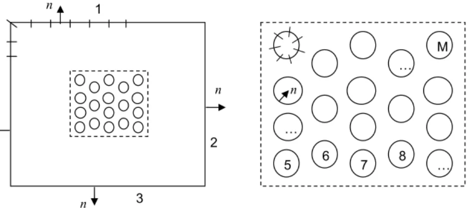
Fig. 1. Schematic presentation of the waveguide containing a porous scatterer constituted by many vertical cylinders in the middle. (a) Top view, (b) vertical

section through the channel centerline.

mangrove trunks and roots are treated as vertical cylindrical elements located in the water column, [7]; see also [8]. Particular arrangements used in experiments and numerical models are regular arrays of vertical cylinders; see e.g., [9–12]. In the case when the scatterer diameter is very small compared to the characteristic wavelength, typically of the order of a few percent, the structure could be macroscopically considered as porous medium. For waves of small steepness the problem is treated in the framework of linear theory. Also, if the length of the porous structure is small, viscous dissipation can be approximately omitted.

For protection structures composed by dense arrays of vertical cylinders, laboratory physical models have been recently used to study and characterize the complex hydrodynamic processes involved during wave propagation within such porous media; see [3]. Furthermore, sloshing experiments in a rectangular tank, completely filled with vertical cylinders undergoing forced horizontal motion around the natural frequency of the first sloshing mode, have been used by Molin and Remy [13] to identify the dispersion equation of linear waves propagating through such dense arrays of vertical cylinders; see also [12]. However, when considering the same porous structures with gaps, as e.g. in periodic arrangements (as in the case of segmented porous breakwaters) or during tests in a rectangular wave tank where the structure occupies the middle region, as studied by Arnaud [14], additional phenomena enter into play, like scattering and interaction with the tank walls, which forms a waveguide, and the appearance of critical frequencies.

When the vertical cylinders in the examined finite-width protection structure extent from the top (free surface) to the bottom surface and the depth is constant, the problem can be treated by the Helmholtz equation on the horizontal plane, supplemented with additional conditions at the sides of the tank or for accounting for the effects of periodic boundaries in the case of segmented porous breakwater. The latter constitutes a scattering problem by many impenetrable bodies in a waveguide. Similar problems are frequently encountered in acoustics, elasticity and electromagnetism; see, e.g., [15–17] and the references cited there. Also, similar applications have been studied by Li and Mei [18] in the case of array of cylinders in a long channel, where multiple scattering can excite Bragg resonances if the frequency falls within one of the band gaps. In this work a coupled numerical scheme, based on a modal expansions, in conjunction with boundary element technique, is developed for treating propagation and scattering by finite structures consisted of regular arrangements of impenetrable cylinders inside a waveguide. Numerical results are presented and discussed concerning the wave details both inside and outside the porous structure, illustrating its applicability operating as breakwater unit in a periodic arrangement. Subsequently, focusing on the reflection and transmission properties far from the structure, a simplified model is derived, based on Foldy–Lax theory; see, e.g., Martin [16]. The latter model provides an equivalent refraction index for the wave scattering by the porous structure located strictly inside the waveguide; see e.g., [19,20]. Results obtained by the present fully coupled and simplified methods are compared against experimental measurements collected in the wave tank of SeaTech of University of Toulon, France, showing good agreement. The present models support further design and optimization studies concerning the examined porous structures, and can be used for studying similar scattering problems in acoustic and electromagnetic waveguides.

2. Mathematical formulation

We consider small-amplitude harmonic water waves of angular frequency

ω

, propagating in the x-direction in a channel or a tank of constant water depth h, with vertical side walls located at y

= ±

d; seeFig. 1. In this environment the waves are scattered by a structure of length L and breadth B, located at the center of the domain. The structure consists of multiple bottom mounted vertical cylinders of radius a

=

D

/

2 in a symmetric arrangement, however, the extension of the present method to treat more general arrangements is straightforward. The above configuration models also the interaction of normally incident waves with a y-periodic arrangement of such structures of breadth B and gaps 2d

−

B between them.

Furthermore, we will consider that the radius of the cylinder(s) is small with respect to the incident wavelength ka

≪

1, where k denotes the characteristic wavenumber

ω

2

₌

_{kg tanh}

₍

_kh

_{) .}

₍₁₎

We consider the multiple scattering problem in the above waveguide excited by any superposition of the incoming propagating modes by

Φ+

(

x

,

y

,

z

;

t

) =

Re

(

Φ+

(

x

,

y

,

z

)

exp

(−

i

ω

t

)) ,

(2)

where i

=

√

−

1 and the complex potentialΦ+

₍

x

,

y

,

z

)

satisfies the Laplace equation and the no-entrance boundary conditions at the bottom z

= −

h and the side walls y

= ±

d. Since the boundaries are vertical surfaces, evanescent modes

corresponding to the imaginary roots of the dispersion relation are not excited and the three-dimensional incident wave potential is given by Φ+

(

x

,

y

,

z

) =

cosh

(

k

(

z

+

h

))

cosh

(

kh

)

Np

∑

n=1 A+_nYn

(

y

)

exp

(

ikxnx

) .

(3)

Considering the above incident field to be symmetric with respect to the centerline (y

=

0) and to satisfy the no-entrance boundary conditions on the side walls

(

y

= ±

d

)

, the transverse eigenfunctions and eigenvalues appearing in the above expansion are given by

Yn

(

y

) =

Wncos

((

n

−

1

)

π

y d

) ,

and kxn

=

√

k2

₋

π

2

₍

_n

₋

₁

₎

2 d2

,

n

=

1

,

2

,

3

, . . .,

(4)

where the constants Wncan be fixed by normalization, and thus,

W1

=

1

/

√

2d and Wn

=

1

/

√

d

,

n

=

2

,

3

, . . . .

(5)

We easily derive from the above relations the number of propagating wavenumbers

Np

=

1

+

[kd

/π

]

,

(6)

where [

◦

] denotes the integer part. It is also seen from the above relations, that for water wavenumbers k

(ω) = (

n

−

1

) π/

d, n

=

2, 3, 4.., which correspond to the following frequencies

ω

n

=

√((

n

−

1

)

g

π/

d

)

tanh

((

n

−

1

) π

h

/

d

),

n

=

2

,

3

. . . ,

(7)

a new mode, with index n, is added to the set of propagating terms. It is seen from Eqs.(3)and(4), that at these frequencies the new mode behaves like a stationary field that could possibly develop a resonance in the waveguide. Furthermore, using Eq.(7), for n

=

1, we obtain the following frequency

ω

1

=

√(

g

π/

d

)

tanh

(π

h

/

d

),

(8)

which identifies the upper limit of frequency for possible excitation of the waveguide only by the first (n

=

1) mode corresponding to plane wave. Thus, for

ω < ω

1the incident field in the waveguide consists only by the parallel wave

Φ+

(

x

,

y

,

z

) =

A₁+cosh

(

k

(

z

+

h

))

cosh

(

kh

)

exp

(

ikx

) ,

(9)

while for higher frequencies,

ω > ω

1, the incident fieldΦ+may contain in general more propagating modes (Eq.(3)).

Using the method of separation of variables complete representations of the wave field are derived in the form of normal mode series; see e.g., [21]. In the upwave region (left semi-infinite strip) the wave field consists of incident, reflected and evanescent components (generated from the scatterer), with amplitudes A(_n1),

Φ(1)

₍

_x

_,

_y

_,

_z

_{) =}

cosh

(

k

(

z

+

h

))

cosh

(

kh

)

⎛

⎝

Np

∑

n=1 A+ nYn

(

z

)

exp

(

ikxnx

) +

∞

∑

n=1 A(1) n Yn

(

y

)

exp

(−

ikxnx

)

⎞

⎠

,

(10a)

while in the downwave region (right half-strip) the field is Φ(3)

₍

_x

_,

_y

_,

_z

_{) =}

cosh

(

k

(

z

+

h

))

cosh

(

kh

)

∞

∑

n=1 A(_n3)Yn

(

y

)

exp

(

ikxnx

) ,

(10b)

and consists only of transmitted and evanescent modes, with amplitudes A(n3).

Since the incident wave field contains only the propagating water-wave modes and the solid boundaries (both side walls of the channel and the multiple scatterers) are vertical surfaces, the evanescent water-wave modes characterized by vertical structure cos

(

kn

(

z

+

h

)) /

cos

(

knh

)

and wavenumbers kn, n

=

1, 2, .. corresponding to the imaginary roots

of the dispersion relation(1)on the complex plane, are not excited. The total three-dimensional field in the considered waveguide contains both the incident and the diffracted component due to structure composed by many vertical cylinders,

Φ

(

x

,

y

,

z

) =

Φ+

(

x

,

y

,

z

) +

Ψ

(

x

,

y

,

z

)

, and is represented by Φ

(

x

,

y

,

z

) = ϕ (

x

,

y

)

cosh

(

k

(

z

+

h

))

cosh

(

kh

)

,

(11a) where

ϕ (

x

,

y

) = ϕ

+

(

x

,

y

) + ψ (

x

,

y

)

and

ϕ

+

(

x

,

y

) =

Np

∑

n=1 A+_nYn

(

y

)

exp

(

ikxnx

) .

(11b)

Thus, the problem is reduced to the Helmholtz equation on the horizontal plane with respect to the surface wave potential

ϕ (

x

,

y

)

(or the free surface elevation

η (

x

,

y

)

) satisfying

(∇

2

₊

_k2

)

ϕ (

x

,

y

) =

0

,

in D

= {−∞

<

x

< ∞, −

d

≤

y

≤

d

}

,

(12a)

∂

n

ϕ (

x

,

y

) =

0

,

(

x

,

y

) ∈ ∂

DC

=

∪

i=1,NC

∂

Di

,

(12b)

∂

y

ϕ (

x

,

y

) =

0

,

y

= ±

d

,

(12c)

ϕ (

x

,

y

) ∼

Np

∑

n=1

A+_nYn

(

y

)

exp

(

ikxnx

) +

reflected waves for x

→ −∞

, −

d

≤

y

≤

d

,

(12d)

ϕ (

x

,

y

) ∼

transmitted waves for x

→ −∞

, −

d

≤

y

≤

d

,

(12e) where

∇ =

(

∂

_x

, ∂

_y

)

is the surface gradient, n indicates the normal vector on the boundary of the NCcylinders (

∂

Di) directed

to the exterior of the fluid domain and

∂

n

ϕ (

x

,

y

)

the corresponding normal derivative of the wave potential on the horizontal

plane.

Some properties of the scattering field

ψ

can be revealed by using the integral representation

ψ (

x

,

y

) ≈

∫

β (

xs

)

G

(

x

|

xs

)

dxs

,

involving the Green’s functionG

(

x

|

xs

)

in the considered waveguide (also termed as a line source), which is given by (see

[21]): G

(

x

|

x0

) =

G

(

x

,

y

|

xs

,

ys

) =

i 2

∑

n=1 Yn

(

y

)

Yn

(

ys

)

exp

(

ikxn

|

x

−

xs

|

)

kxn

,

where x

=

(

x

,

y

)

denotes the field point and xs

=

(

xs

,

ys

)

the corresponding source with density

β

, respectively. From

the above it is seen that at the critical frequencies specified by Eq.(9), the x-wavenumbers kxn

=

0 (see Eq.(4)), and if

these modes are excited, the scattering field could possibly become singular resonating the waveguide. Before proceeding to the reformulation of the problem, Eqs.(12), as a matching boundary value problem based on the fundamental solution of the Helmholtz equation (or the free-space Green’s function), it is worth mentioning here that the above complex Green’s function is slowly convergent, especially near the singularity as the field point (x, y) approaches the source point (xs

,

ys).

This fact leads to increased computational complexity and cost, especially concerning the calculation of the BEM influence coefficients. On the other hand, the evaluation of the latter quantities using the free-space Green’s function is much easier and faster, at the cost of increased discretization required due to the treatment of additional boundaries (the side walls and the matching interfaces) that need to be considered.

Using Eqs.(10), the above multiple scattering problem in the infinite strip

−∞

<

x

< ∞

,

−

d

≤

y

≤

d, is reformulated

interior the Nccylindrical scatterers, as follows:

(∇

2

₊

_k2

)

ϕ

(2)

₍

_x

_,

_y

_{) =}

₀

_,

_{in D}(2)

_{−

_{ℓ <}

_x

_{< ℓ , −}

_d

_≤

_y

_≤

_d

_}

_,

_(13a)

∂

n

ϕ

(2)

(

x

,

y

) =

0

,

(

x

,

y

) ∈ ∂

DC

,

(13b)

∂

y

ϕ

(2)

(

x

,

y

) =

0

,

−

ℓ <

x

< ℓ ,

y

= ±

d

,

(13c)

ϕ

(2)

₍

_x

_,

_y

_{) = ϕ}

(1)

₍

_x

_,

_y

₎

_and

_∂

x

ϕ

(2)

(

x

,

y

) = ∂

x

ϕ

(1)

(

x

,

y

) ,

x

= −

ℓ, −

d

≤

y

≤

d

,

(13d)

ϕ

(2)

₍

_x

_,

_y

_{) = ϕ}

(3)

₍

_x

_,

_y

₎

_and

_∂

x

ϕ

(2)

(

x

,

y

) = ∂

x

ϕ

(1)

(

x

,

y

) ,

x

=

ℓ, −

d

≤

y

≤

d

,

(13e)

where x

= ±

ℓ

denotes the position of the interfaces shown also by using dotted lines inFig. 1(a), and

ϕ

(1)

₍

_x

_,

_y

_{) =}

Np

∑

n=1 A+_nYn

(

y

)

exp

(

ikxnx

) +

∞

∑

n=1 A(_n1)Yn

(

y

)

exp

(−

ikxnx

) ,

(14a)

ϕ

(3)

₍

_x

_,

_y

_{) =}

∞

∑

n=1 A(_n3)Yn

(

y

)

exp

(

ikxnx

) .

(14b)

We note that all terms in the above infinite series with index greater than Nppresent exponential decay (always faster

for larger n) because the wavenumbers kxndefined from Eq.(4)are imaginary always increasing in modulus. In the sequel

the series appearing in the above equations are truncated keeping only a finite number Nmof terms (Nm

>

Np) that are

sufficient for numerical convergence.

Given the amplitudes of the incident modes

{

A+

n

,

n

=

1

,

2

, . . . ,

Np

}

, the problem is solved in the box-shaped bounded subregion (

−

ℓ <

x

< ℓ

,

−

d

≤

y

≤

d), finding the unknown wave potential

ϕ

(2)_{and the sets of unknown coefficients} A(n1)

,

A(

3)

n , n

=

1, 2, . . . . In the following, a hybrid modal-BEM will be presented for treating the above problem. For simplicity

in the presentation, from now on the wave in the middle region

ϕ

(2)

(

x

,

y

)

will be simply denoted as

ϕ (

x

,

y

)

and the corresponding domain as D.

Moreover, energy flux conservation is easily derived by using Green’s theorem for the field in the waveguide, in conjunction with the wall conditions Eqs.(12c), from which we finally obtain

Im

{∫

y=d y=−d

ϕ

∗

(

x

,

y

)

d

ϕ (

x

,

y

)

dx dy

}

=

const

,

(15a)

for any transverse section x

=

const of the waveguide outside the scatterer, where

ϕ

∗

denotes the complex conjugate of the potential. Applying the above equation, in conjunction with the representations(14)in the far upwave region x

≪ −

ℓ

and in the far downwave region x

≫ −

ℓ

, and using the fact that the functions

∥

Yn

∥ =

1, the following relation is derived:

Np

∑

n=1 kxn

(

⏐

⏐

A + n

⏐

⏐

2

−

⏐

⏐

A(_n1)

⏐

⏐

2

)

=

Np

∑

n=1 kxn

⏐

⏐

A(_n3)

⏐

⏐

2

.

(15b)

The above relation will be used to check satisfaction of energy conservation from the calculated values of the reflection and transmission amplitudes, as obtained by the present modal-BEM that will be described in detail in the next sections.

3. The matching-boundary value problem

In the bounded (middle) subregion the wave field is represented by a single layer boundary integral representation based on simple sources, as follows

ϕ (

x

) =

∫

∂D

σ (

x_s

)

G

(

x

|

x_s

)

ds

(

x_s

) ,

x

∈

D

∪

∂

D

,

(16a) where x

=

(

x

,

y

)

denotes the field point, xs

=

(

x

,

y

) ∈ ∂

D the source point on the boundary, and the involved function

G

(

x

|

xs

)

is the fundamental solution of Helmholtz equation on the plane, which should not to be confused with the Green’s

function G

(

x

|

xs

)

of the previous section. The fundamental solution is defined by means of the Hankel function of zero order

and first kind as follows

G

(

x

|

xs

) =

i

4H

(1)

Fig. 2. Hybrid modal-BEM formulation and discretization of various sections of the boundary in the middle subdomain of the waveguide. Side walls are the

boundary parts 1 and 3, and the incident and transmission interfaces are the parts 4 and 2, respectively. The cylindrical scatterers are numbered as parts 5, 6, . . . , M. Also, the outward normal vector on various parts of the boundary is indicated.

Using the jump relations of the single layer we obtain from Eqs.(16)the following integral representations concerning the derivatives of the potential

∇

ϕ =

⎧

⎪

⎪

⎨

⎪

⎪

⎩

∇

_x

∫

∂D

σ (

xs

)

G

(

x

|

xs

)

ds

(

xs

) =

∫

∂D

σ (

xs

) ∇

xG

(

x

|

xs

)

ds

(

xs

) ,

for x

∈

D

σ (

x

)

n 2

+

∫

∂D

σ (

xs

) ∇

xG

(

x

|

xs

)

ds

(

xs

) ,

for x

∈

∂

D (17)

Then by calculating the wave velocity for points on the boundaryx

∈

∂

D we obtain the representation of the normal

derivative of the potential

∂ϕ

∂

n

⏐

⏐

⏐

⏐

∂D

≡

n

∇

ϕ =

σ (

x

)

2

+

∫

∂D

σ (

xs

) ∂

nG

(

x

|

xs

)

ds

(

xs

) ,

x

∈

∂

D

,

(18)

where n denotes the unit normal vector on the boundary (directed outwards the domain D), as shown inFig. 2, and

∂

nG

(

x

|

xs

) =

n

∇

xG

(

x

|

xs

)

. Then, the Neumann boundary condition on the solid boundary of the scatterers and the side

walls is

σ (

x

)

2

+

∫

∂D

σ (

xs

) ∂

nG

(

x

|

xs

)

ds

(

xs

) =

0

,

for x

∈

∂

DC and

−

ℓ <

x

< ℓ ,

y

= ±

d

.

(19)

The formulation is completed by including the matching condition at the two interfaces separating the middle domain

D from the two semi-infinite strips. To this aim using the truncated versions of Eqs.(14)keeping only a finite number Nm

of terms Nm

>

Np, and the boundary integral representations(16)and(17), we obtain for points x on the left interface

{

x

= −

ℓ, −

d

≤

y

≤

d

}

the following equation expressing the matching of the potential

ϕ|

x=−_ℓ

≡

∫

∂D

σ (

xs

)

G

(

x

|

xs

)

ds

(

xs

) =

Np

∑

n=1 A+_nYn

(

y

)

exp

(

ikxn

ℓ) +

Nm

∑

n=1 A(_n1)Yn

(

y

)

exp

(−

ikxn

ℓ) ,

(20)

and as concerns the matching of the normal derivative

∂ϕ

∂

n

⏐

⏐

⏐

⏐

x=−_ℓ

≡

σ (

x

)

2

+

∫

∂D

σ (

xs

) ∂

nG

(

x

|

xs

)

ds

(

xs

)

= −

Np

∑

n=1 ikxnA + nYn

(

y

)

exp

(

ikxn

ℓ) +

Nm

∑

n=1 ikxnA(n1)Yn

(

y

)

exp

(−

ikxn

ℓ) .

(21)

Using the orthogonality and completeness properties of the basis functions

{

Yn

(

y

) ,

n

=

1

,

2

, . . .}

in the interval

−

d

≤

y

≤

d, the coefficients

{

A(n1)

,

n

=

1

,

2

. . .

}

are expressed from Eq.(20)as follows

A(_n1)

=

exp

(

ikxn

ℓ) (⟨ϕ|

x=−ℓ

,

Yn

⟩ −

A

+

n exp

(

ikxn

ℓ)) ,

n

=

1

,

2

,

3

. . . ,

(22)

Using the above result in Eq.(21)we obtain the final form of the non-local boundary condition expressing the matching of the potential on the left interface x

= −

ℓ

:

∂ϕ

∂

n

⏐

⏐

⏐

⏐

x=−_ℓ

−

Nm

∑

n=1 ikxn

⟨

ϕ|

x=−ℓ

,

Yn

⟩

Yn

(

y

) = −

2ikxnA + n exp

(

ikxn

ℓ)

Yn

(

y

) , −

d

≤

y

≤

d

,

(23) where A+

n is the n-amplitude of the incident mode constituting the forcing of the problem. Quite similarly, for points on

the right interface

{

x

=

ℓ, −

d

≤

y

≤

d

}

we obtain the following result concerning the coefficients of the expansion of the potential in the right half strip

A(_n3)

=

exp

(−

ikxn

ℓ) ⟨ϕ|

x=ℓ

,

Yn

⟩

,

n

=

1

,

2

,

3

. . . .

(24)

and using this result we obtain the following non-local condition, expressing the matching of the potential on the right interfacex

=

ℓ

:

∂ϕ

∂

n

⏐

⏐

⏐

⏐

x=_ℓ

−

Nm

∑

n=1 ikxn

⟨

ϕ|

x=ℓ

,

Yn

⟩

Yn

(

y

) =

0

, −

d

≤

y

≤

d (25) where

ϕ|

x=−ℓ

≡

∫

∂D

σ (

xs

)

G

(

x

|

xs

)

ds

(

xs

)

and

∂ϕ

∂

n

⏐

⏐

⏐

⏐

x=−ℓ

≡

σ (

x

)

2

+

∫

∂D

σ (

xs

) ∂

nG

(

x

|

xs

)

ds

(

xs

)

considered for points

{

x

=

ℓ, −

d

≤

y

≤

d

}

.

The examined problem possesses a unique solution, with the possible exception of a set of discrete frequencies constituting the spectrum of irregular frequencies connected with the single layer representation used; see, e.g., [22,23] and the references cited there. Also, the possible existence of trapped modes at specific frequencies could cause non-uniqueness of the problem (see, e.g., [24]). In the present work we focus on the numerical solution of the above system in the case of regular frequencies only, leaving the study of the interesting problem concerning irregular frequencies and singular conditions in future extensions.

4. The modal Boundary Element Method

The problem is solved by applying a Boundary Element Method to calculate the integral operators, in conjunction with a collocation technique. The external boundary of the middle domain consists of four parts (walls, incidence and transmission sides) and the boundaries of discs in the arrangement, numbered consecutively as indicated inFig. 2. Moreover, linear elements are used to discretize the various parts of the boundary, ensuring continuity of geometry, in conjunction with a piecewise constant approximation of the source distribution

σ (

x

) ,

x

∈

∂

D. Thus, the unknowns are the value of the

density in each element

σ

j

,

j

=

1

,

2

, . . . ,

Nel, where Nelis the total number of elements used to discretize all parts of the

boundary, and the equations are satisfied at specific control points xj

∈

∂

D, selected to be the centers of the boundary

elements, j

=

1

,

2

, . . . ,

Nel; seeFig. 2. In this way, the integrals representing the values of the potential and its normal

derivative on the boundary involved in the boundary and matching conditions Eqs.(19),(23)and(25), are approximated by

ϕ (

xj

) =

Nel

∑

n=1

σ

nFjn

,

∂

n

ϕ (

xj

) =

Nel

∑

n=1

σ

nUjn

.

(26)

In the above relations, the matrices Fjnand Ujnare defined by the following integrals defining induced quantities from

the n-linear element to the j-control point, respectively,

Fjn

=

∫

(n) H₀(1)

(

k

⏐

⏐

x_j

−

x

(

s

)⏐⏐)

ds

,

(27) and Ujn

=

δ

jn 2

−

k

∫

(n) H₁(1)

(

k

⏐

⏐

xj

−

x

(

s

)⏐⏐)

nx_n

(

xj

−

x

(

s

)) +

nyn

(

yj

−

y

(

s

))

⏐

⏐

xj

−

x

(

s

)⏐⏐

2 ds

.

(28)

In the above equations x

(

s

) = (

x

(

s

) ,

y

(

s

))

denotes the parametric equation of the n-element with s denoting the physical length, n

=

(

nx_j

,

ny_j

)

is the outer unit normal vector at the center of the j-element, and H₁(1)is the Hankel function of first kind and first order. For j

̸=

n the integrals in Eqs.(27)and(28)are regular and, for small nondimensional wavenumbers k

δ

s,

where

δ

s is a representative value of the meshsize on the boundary (element length), and small distances k

⏐

⏐

x_j

−

x_n

⏐

⏐

, they can

be calculated by usual numerical integration rules, and in the present work an adaptive Simpson’s rule is applied. Difficulties could arise for higher frequencies, which is the case in similar problems in acoustic and electromagnetic waveguides, where these integrals are more efficiently calculated by means of Filon’s rule; see, e.g. [25]. For large distances k

⏐

⏐

x_j

−

x_n

⏐

⏐ ≫

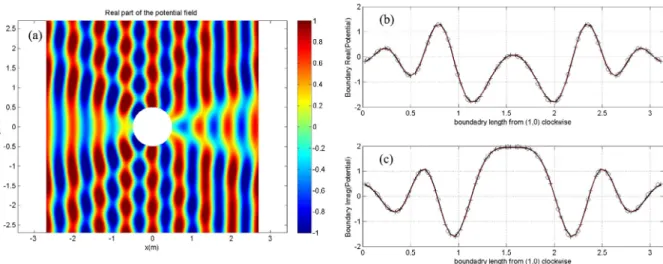
1, the

Fig. 3. (a) Waves scattered by a hard cylinder (ka=4.66) as calculated by the present BEM using Nel=31 elements. (b) Real part of the potential on the

surface of the cylinder using Nel=31 (circles), Nel=61 (crosses) against the analytical solution (solid lines). (c) Same as before for the imaginary part of

the potential.

the other hand, for j

=

n the integral in Eq.(27), expressing the induced potential from a linear element to its center, is weakly singular. These integrals contain logarithmic singularity and are conveniently treated by transformation of the integration variable. In particular, simple transformations of the form u2

₌

₍

_s

₋

_s

mid

)

, where smidthe coordinate of the middle of the

element, bringing the integration points closer to the singularity, are sufficient in order to reduce the integrals to regular ones and apply similar as before numerical rules. Finally, we notice that for j

=

n the singular integral in Eq.(28)exists in the sense of Cauchy principal value. However, it becomes simply zero due to symmetry properties of the kernel about the point of singularity. The above facts result in a very fast calculation of the matrices Fjnand Ujneven for complex configurations

discretized by using large number of elements.

On the basis of the above, the boundary condition Eq.(19)on the surface of the scatterers

∂

DC and on the side walls

y

= ±

d, becomes

Nel

∑

n=1

σ

nUjn

=

0

,

for j

∈ {

J

(∂

Dc

) ,

J

(

y

= ±

d

) } ,

(29)

where J

(∂

Dc

) ,

J

(

y

= ±

d

)

denote the corresponding set of indices of the panels on these parts of the boundary

∂

D. The

infinite series appearing in Eqs.(23)and(25), respectively, are truncated keeping only a finite number of terms Nm

>

Np,

exploiting the fact that all terms above Nppresent exponential decay (always faster for larger n) because the wavenumbers

kxndefined from Eq.(4)are imaginary always increasing in modulus. Furthermore, using the BEM representations(26)in

Eqs.(23)and(25)we obtain:

Nel

∑

n=1

σ

nUjn

−

i Nm

∑

n=1 kxnYn

(

yj

)

Nel

∑

p=1

σ

pFmp

⟨

Hm

,

Yn

⟩ = −

2ikxn

(

δ

nmA + m

)

exp

(

ikxn

ℓ)

Yn

(

yj

)

,

p

,

m

,

and j

∈

J

(

x

= −

ℓ) ,

(30) Nel

∑

n=1

σ

nUjn

−

i Nm

∑

n=1 kxnYn

(

yj

)

Nel

∑

p=1

σ

pFmp

⟨

Hm

,

Yn

⟩ =

0

,

p

,

m

,

and j

∈

J

(

x

=

ℓ) ,

(31)

where Hm

(

y

)

denotes the unit step function with support on the m-element of the vertical interfaces. Clearly, the above

equations materialize the discrete form of the matching-boundary conditions by the present modal-BEM formulation, and the linear system is solved with respect to the discrete complex unknowns

{

σ

_n

,

n

=

1

,

2

, . . . ,

Nel

}

.

4.1. Validation in the case of scattering of parallel incident waves by hard cylinder

In order to illustrate the applicability and efficiency of the present method, we first consider the simple case of scattering of plane harmonic waves by a single hard cylindrical scatterer in infinite domain, corresponding to the limiting case of waveguide of infinite width (d

→ ∞

). This will help us also to estimate the number of panels on each cylinder that is needed for convergence of the results.

Fig. 4. Porous breakwater constructed by regular arrangement of vertical cylinders.

In this case analytical solution is available, which is obtained by separation of variables in cylindrical coordinates. Assuming that the circular scatterer of radius a is located at the center of the domain

(

x

,

y

) = (

0

,

0

)

, the analytical solution is given by (see, e.g., [16,27]),

ϕ (

r

, θ) =

exp

(

ikx

) + ψ (

r

, θ) ,

(32a)

ψ (

r

, θ) =

∞

∑

m=0 Amcos

(

m

θ)

Hm(1)

(

kr

) ,

with Am

= −

ε

mim J′ m

(

ka

)

Φ(1) m

(

ka

)

,

(32b) where r

=

(

x2

₊

_y2

)

1/2

, θ =

2 tan−1

₍

_y

_/(

_x

₊

_r

₎₎

_{are the cylindrical coordinates and J}′

m

(

u

) =

dJm(u) du andΦ (1) m

(

u

) =

dH( 1) m (u) du ,

and

ε

mis the Neumann symbol (

ε

m

=

1

,

m

=

0

,

and

ε

m

=

2

,

m

≥

1). Indicative results obtained by the present BEM are

shown inFig. 3for Nel

=

31 and 61 elements on the surface of the impermeable cylinder and compared against the analytical

solution. In this example, we consider plane water waves of frequency f

=

1.5 Hz propagating in constant depth h

=

0.23 m, and thus, the shallowness parameter is h

/λ =

0

.

34 corresponding to intermediate water depth. The waves are scattered by a circular, bottom mounted cylinder of radius a

=

0.5 m, which is comparable to the dimensions of the porous structure examined in this work as presented in more detail in the next section. Thus, the nondimensional wavenumber in the case of

Fig. 3is ka

=

4

.

66. We clearly observe the excellent convergence of the present BEM scheme to the analytical solution.

4.2. Numerical results for the many cylinder structure in the waveguide

In recent research by Arnaud et al. [3] wave propagation through arrangements of vertical cylinder arrays is investigated, that is examined for possible applications as permeable breakwaters and protective structures. In particular, laboratory physical models have been systematically tested in [14] to characterize the complex hydrodynamic processes involved during wave propagation and to study the effect of specific surface or porosity on the wave energy dissipation; seeFigs. 4and5. Several arrangements with different cylinder diameters have been considered in order to study the effects of the specific surface while keeping the porosity constant. In particular, three cylinder diameters are considered in [14], with

D

=

0.020 m, 0.032 m and 0.050 m, arranged in blocks of length L

=

0.3 m and breadth B

=

1.2 m. The cylinders are regularly disposed along two perpendicular axes forming a 45 deg angle with the longitudinal axis. Porosity in the case of the examined arrangements of vertical cylinders attain the same value, given in terms of diameter D and number NC of

cylinders as follows:

γ =

1

−

NC

π

a2

LB

,

where a

=

D

/

2

.

(33)

The structure ofFig. 4with cylinders of diameter D

=

0.032 m and the indicated spacing is modeled by arranging 17 rows of 4 cylinders in x direction and, between them, 16 rows of 5 cylinders, i.e. a total number Nc

=

148 cylinders, as shown inFig. 6. Using the above values in Eq.(33)it results in

γ =

0

.

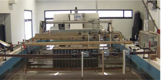
67 which approximates well the reported value in the experiments [3,14]. Although the above value of porosity is relatively low, the term ‘dense arrays of vertical cylinders’ is also used herein to characterize this type of structures; see also [12].

Fig. 5. Tests in the wave tank of Seatech (Univ. Toulon) with the porous breakwater unit located in the middle of the tank.

Table 1

Critical frequencies of Seatech tank, for water depth h=0.23 m and distance between centerline and side walls d=1.3 m.

n 1 2 3 4 5 6

fn(Hz) 0.55 0.98 1.29 1.53 1.72 1.89

The above structure operating as porous segmented breakwater is tested in the wave tank of Seatech shown inFig. 5, in water depth h

=

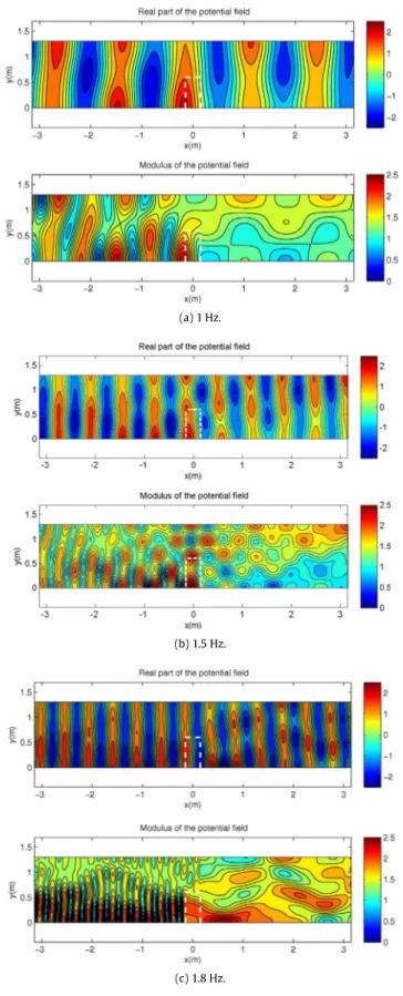
0.23 m. The tank is 10 m long and 2.6 m wide, and the porous breakwater is located in the middle of the tank so that the side gaps between the structure and the walls of the tank are equal to 0.7 m. For this configuration and water depth the critical frequencies estimated from Eq.(7)are listed inTable 1below.

In the following, we consider forcing only by the first incident mode (plane incident waves) in the tank, and results obtained by the present modal-BEM are shown inFig. 6for three frequencies f

=

1 Hz, 1.5 Hz and 1.8 Hz, for which experiments were performed in the tank. Present calculations are based on total M

=

152 boundary sections modeling the waveguide and all the cylinders in the porous structure. More specifically, 50 elements are used along the side walls and 64 elements in the entrance and exit boundaries. Also, 30 elements are used to discretize each one of the 148 cylinders in the arrangement, resulting in a total number of 4668 elements, which is found enough for numerical convergence. In the colorplots ofFig. 6(left column) the real part and the modulus of the wave field, at each one of the above frequencies, is shown. In all cases we observe that the field is resolved with high accuracy, both outside and inside the arrangement of vertical cylinders composing the porous structure. In the right subplots ofFig. 6the computed results along the section

y

=

0.1 m (at 10 cm from the centerline of the tank) are shown. The real part of the wave field is plotted by using thin solid line and the imaginary part by dashed line, respectively. Also, the modulus of the wave field, which is proportional to the distribution of the amplitude of the free-surface elevation along the same longitudinal section, is shown by using thick lines. In these plots, the limits of the structure are indicated by vertical dashed lines. We observe that at all frequencies the structure allows much part of the flow and energy to be transmitted to the downwave side. In particular, as concerns energy transmission, the examined structure seems to be more efficient at lower frequencies. Furthermore, although in cases (a) and (b) the frequency (f

=

1 Hz and 1.5 Hz) is close to the second and fourth critical value (seeTable 1), respectively, still no special effect is reflected in the results, indicating that the possible resonances are very local.

For the examined configuration, more results concerning the reflection and transmission of waves are presented inFig. 7, characterizing also the energy exchange between the first incident mode (with amplitude A+₀) and the higher modes that can be excited by the scattering structure in the tank, as the frequency exceeds the critical values ofTable 1. In this figure the nondimensional coefficients associated with the reflection and the transmission modes are plotted, as calculated by the present modal-BEM. These coefficients are defined by the corresponding amplitudes in the representations, Eqs.(14a)and

(14b), respectively, as follows Rn

=

⏐

⏐

A(_n1)

⏐

⏐

/

A + 0

,

and Tn

=

⏐

⏐

A(_n3)

⏐

⏐

/

A + 0

,

n

=

1

,

2

,

3

, . . . .

(34)

In particular, the first three coefficients, containing most of the energy, are plotted against the nondimensional wavenumber

kh

=

2

π

h

/λ

, for frequencies from 0.8 to 2.1 Hz, corresponding to wave conditions ranging from intermediate water depth to deep water. We observe inFig. 7, similarly as in the case of finite underwater steps or submerged breakwaters, that the behavior of transmission and reflection coefficients presents alternating maxima and minima at specific frequencies.

Fig. 6. Calculated wave field (only half symmetric part) in the waveguide modeling the tank experiments in water depth h=0.23 m, at frequencies (a)

f=1 Hz, (b) f =1.5 Hz, (c) f=1.8 Hz, excited by the first incident mode. The right column subplots indicate computed results along the section y=0.1 m from the centerline. Real part of the field is indicated by thin solid line, imaginary part by dashed line, and modulus with thick lines, respectively. The limits of the structure are indicated by vertical dashed lines.

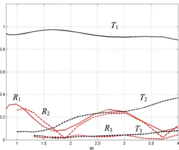
Fig. 7. Transmission coefficients (Tn, shown by using black lines) and reflection coefficients (Rn, shown by using red lines) of the examined porous structure

against nondimensional wavenumber kh, concerning the first three modes. Results for the first mode are indicated by using solid lines and for the rest by dashed lines, respectively. (For interpretation of the references to color in this figure legend, the reader is referred to the web version of this article.)

Moreover, as the frequency of the incident wave increases, higher modes are excited, carrying energy in the transmission region. We also remark here that the shown results, obtained by using the above discretization, are found to be consistent with the energy conservation relation Eq.(15b), presenting error less than 1%, which diminishes with further increase of the number of boundary elements.

In the following, we will consider the above as reference data to compare with results obtained by a simplified model and experimental measurements in the tank. The computational cost of the simplified model is significantly less that the above more complete modal-BEM solution, facilitating its systematic application to investigate the reflection and transmission properties of such porous structures in more complex environment and supporting further design and optimization studies. Comparative data for computational requirements and time will be provided at the end of Section5.2.

5. A simplified coupled-mode model on the horizontal plane

In the case of the scattering of time-harmonic waves by large number of densely arranged small obstacles in a homogeneous medium, where the size of the bodies is quite small compared with the wavelength, the computation cost of the numerical simulation of the field by boundary element methods, in conjunction with a Dirichlet-to-Neumann conditions, can become excessively high, making difficult its use in optimization studies and application to scattering problems by many such structures in realistic environments. In this section an approximate, simplified model, with very low computational requirements, is presented and tested for the solution of the problem. The simplified model is based on the Helmholtz equation on the horizontal plane, and treats the porous structure as an inclusion in the waveguide, characterized by an effective index of refraction keff. The latter is estimated as discussed in more detail inAppendixby an adapted version

Foldy–Lax theory (see, e.g., [16]). Thus, the governing equation is

(∇

2

₊

_κ

2

)

ϕ (

x

,

y

) =

0

,

(35)

where the wavenumber parameter in the water subregion is the standard one

κ

2

₌

_k2_{(as obtained from Eq.(1)for the given}

frequency and water depth), and in the porous subregion this parameter is approximated by an effective value as follows,

κ

2

₌

_k2

eff

=

γ

k

2

_,

₍₃₆₎

where

γ

is the porosity coefficient (defined by Eq.(33)).

The solution of the Helmholtz equation(35)is obtained by a domain decomposition technique. The problem is solved taking into account the incidence-reflection condition at the entrance and the transmission condition at the exit of the waveguide, the side-wall boundary conditions, and the matching conditions on the interfaces separating the porous from the water subregions, shown by using dashed lines inFig. 8. The usual interface conditions (see, e.g., [21]) concern the normal derivative

∂ϕ/∂

n and the value of the wave field

ϕ (

x

,

y

)

on the two sides of the interface. In the present work we use the following conditions

∂ϕ

∂

n

⏐

⏐

⏐

⏐

_w ater

=

γ

∂ϕ

∂

n

⏐

⏐

⏐

⏐

porous

,

(37)

Fig. 8. Domain decomposition of the plane waveguide including the porous structure (porous region) in the middle part shown by thick dashed lines.

which expresses the interface condition for the flow rate through the interface (see, e.g., [1], Eq. 2.14), in conjunction with

ϕ|

water

=

S

ϕ|

porous

,

(38)

which expresses the interface condition for the pressure across the same interface, where S is an empirically estimated coefficient (see, e.g., [1], Eq. 2.13). It is remarked here that in several works concerning the propagation of water waves through or over porous media, see e.g., [1,2,28], the model by Sollitt and Cross [29] is used to describe the porous flow. In the latter model an extra term is included in the momentum equation representing the effect of added resistance caused by the virtual mass of the grains in the porous medium, and when applied to the present configuration it results to a modification of the water-wave dispersion relation, as follows

ω

2_S

₌

_k pg tanh

(

kph

)

,

(39)

from which the wavenumber kpassociated with the propagating mode in the porous subregion can be calculated. In the

latter works S

=

1

+

CM

(

1

−

γ ) /γ

is described as a coefficient representing the effect of inertia in the porous flow. The

inertia coefficient CMfor circular discs, especially in the frequency band and corresponding Reynolds numbers (wave inertial

to viscous forces) considered here, takes values near unity. Thus, in the present case S

≈

1

/γ >

1 and the wavenumber in the porous subregion derived from Eq.(39)would be kp

>

k. Furthermore, theoretical and experimental analysis involving

sloshing experiments by Molin & Remy (2016) [13], shows that the following modified form of the dispersion relation better describes the wave properties in the porous region

ω

2

√

_S

₌

_k pg tanh

(

kph

/

√

S

) ,

(40)

which results in kp

=

k

/√γ

, and thus also kp

>

k. Therefore, for S

>

1, both the above dispersion relations Eqs.(39)and (40), produce values for the wavenumber kpthat are greater than the corresponding value k in the water region (for the same

frequency), and the appropriate use of the dispersion relation to represent the waves over the porous region is thoroughly discussed in [12]. On the other hand, in the present simplified model the wave parameter in the porous subregion is smaller than the water wavenumber, keff

=

√γ

k

<

k. However, it should be stressed here that keff is not representative of the water

wave behavior over the porous structure, but rather it provides us with an effective index of refraction for modeling the scattering effect of the porous structure treated as an inclusion on the basis of applications based on the Helmholtz equation on the horizontal plane. In the sequel a coupled-mode system will be presented for solving the above problem Eqs.(35)–(38)

and approximating the performance of the porous structure with very small computation cost.

5.1. Coupled-mode system

On the basis of coupled mode theory, the problem is approximately solved on the horizontal plane by decomposing the domain into three parts denoted by (I), (II) and (III) inFig. 8, where (I) and (III) are incident and transmission water subregions in the waveguide and the field is provided by the expansions(14a)and(14b), respectively. In the middle subdomain (II), which includes the porous medium modeling the structure, a similar modal expansion is introduced, as follows

ϕ

(2)

₍

_x

_,

_y

_{) =}

∑

n=1

ϕ

n

(

x

)

Yn(2)

(

y

) ,

−

ℓ ≤

x

≤

ℓ , −

d

≤

y

≤

dp and dp

≤

y

≤

d

,

(41)

where the new functions

{

Yn(2)

(

y

) ,

n

=

1

,

2

, . . . .

}

are symmetric, Yn(2)

(

y

) =

Yn(2)

(−

y

)

, in

−

d

≤

y

≤

0 and 0

≤

y

≤

d,

respectively, and are obtained as the solution of the following eigenvalue problem in 0

≤

y

≤

d : d2_Y(2) n

(

y

)

dy2

+

(

k2

(

y

) −

k2_n

)

Y_n(2)

(

y

) =

0

,

in 0

<

y

<

d

,

(42a)

Fig. 9. First four vertical eigenfunctions Yn(y), in 0<y<d=1.3 m, in the case of f =1.8 Hz, h=0.23 m, for: (a)γ =S=1 in uniform layer (e.g., in

water regions I and III), (b) in the middle subregion (II), forγ =0.67 and S=1/γ, and (c)γ =0.67 and S=1, with the interface located at y=dp=0.6 m,

as indicated by horizontal dashed line. The lower part (P) denotes porous medium and the upper part (W) water, respectively.

dYn(2)

(

y

)

dy

=

0

,

y

=

0 and y

=

d

,

(42b) Y_n(2)

(

y

=

dp

+

0

) =

SYn(2)

(

y

=

dp

−

0

)

,

(42c) dYn(2)

(

y

=

dp

+

0

)

dy

=

γ

dYn(2)

(

y

=

dp

−

0

)

dy

,

(42d) where

k2

(

y

) =

k2 for d

>

y

>

dp and k2

(

y

) =

k2eff for 0

<

y

<

dp

.

(42e)

The eigenfunctions associated with the above problem are given by

Y_n(2)

(

y

) =

W cos

(√

k2 eff

−

k2ny

) ,

in 0

<

y

<

dp

,

(43a) Y_n(2)

(

y

) =

W cos

(

√

k2

₋

_k2 ndp

)

cos

(

_√

k2

₋

_k2 n

(

d

−

dp

)

)

cos

(√

k2

₋

_k2 n

(

d

−

y

)

)

,

in d

>

y

>

dp

,

(43b)

and the constant W can be again fixed by normalization. In the sequel the above eigenfunctions will be simply denoted as Yn

(

y

) =

Yn(2)

(

y

) /







Y (2) n







, and since they are orthogonal it holds

⟨

Yn

,

Ym

⟩ =

δ

nm, where

δ

nmdenotes Kronecker’s delta.

Moreover, the corresponding eigenvalues

{

kn

,

n

=

1

,

2

, . . .}

are determined by the roots of the following equation

γ

√

k2 eff

−

k2nsin

(√

k2 eff

−

k2ndp

)

cos

(√

k2

₋

_k2 n

(

d

−

dp

)

)

+

S

√

k2

₋

_k2 nsin

(√

k2

₋

_k2 n

(

d

−

dp

)

)

cos

(√

k2 eff

−

k2ndp

)

=

0

.

(44)

InFig. 9the first four vertical eigenfunctions Yn

(

y

)

, in 0

<

y

<

d

=

1

.

3 m, are plotted, for frequency f

=

1.8 Hz and

water depth h

=

0.23 m. In particular three cases of porosity coefficients are examined: (a)

γ =

S

=

1 in uniform layer (e.g., in water regions I and III), (b) for

γ =

0

.

67 and S

=

1/

γ

, and (c)

γ =

0.67 and S

=

1. In all cases the interface is located at

y

=

dp

=

0

.

6 m, and is indicated by using horizontal dashed lines. In the last two cases ofFig. 9(b) and (c) the discontinuities

concerning the eigenfunctions and its y-derivative are evident at the interface separating the lower part corresponding to the porous (P) medium and the upper part corresponding the water (W) region, respectively.

Consequently, in the present simplified model, the problem is solved by finding the modal amplitudes

ϕ

n

(

x

)

in order to

satisfy Helmholtz equation in subregion (II)

∇

2

ϕ

(2)

+

k2

(

y

) ϕ

(2)

=

0

,

(45)

in conjunction with the following matching conditions

∂ϕ

(1)

∂

x

=

N

(

y

)

∂ϕ

(2)

∂

x and

ϕ

(1)

₌

_F

₍

_y

_{) ϕ}

(2) _{on 0}

_<

_y

_<

_d

_,

_x

_{= −}

_ℓ,

_(46a)

∂ϕ

(3)

∂

x

=

N

(

y

)

∂ϕ

(2)

∂

x and

ϕ

(1)

₌

_F

₍

_y

_{) ϕ}

(2) _{on 0}

_<

_y

_<

_d

_,

_x

₌

_ℓ,

_(46b)

where

ϕ

(1)_and

_ϕ

(3)_{are given by the modal expansions, Eqs.(14), in subregions (I) and (III), respectively. Also, the functions}

N

(

y

)

and F

(

y

)

are determined from parameters

γ

and S as follows:

N

(

y

) = γ ,

for 0

<

y

<

dp and N

(

y

) =

1

,

for dp

<

y

<

d

,

(47a)

and

F

(

y

) =

S

,

for 0

<

y

<

dp and F

(

y

) =

1

,

for dp

<

y

<

d

.

(47b)

Subsequently, by projecting Eq.(45), at each position x, on the transverse basis

{

Yn

(

y

) =

Yn(2)

(

y

) /







Y (2) n





 ,

n

=

1

,

2

, . . .

}

, the following system of horizontal equations is derived with respect to the (unknown) modal amplitudes

ϕ

n

(

x

) ,

in

−

ℓ <

x

< ℓ

,

∑

n amn

ϕ

′′ n

+

cmn

ϕ

n

=

∑

n

δ

mn

(

ϕ

′′ n

+

k 2 n

ϕ

n

) =

0

,

n

=

1

,

2

,

3

, . . . ,

(48)

where a prime denotes differentiation with respect to x, and the coefficients of the system are defined by

amn

= ⟨

Yn

,

Ym

⟩ =

δ

mn and cmn

=

⟨

∂

2_Y n

∂

y2

+

k 2

₍

_y

₎

_Y n

,

Ym

⟩

=

k2_n

δ

mn

.

(49)

Moreover, the following boundary conditions are derived from the matching conditions, Eqs.(46),

∑

n Amn

ϕ

n′

(

x

= −

ℓ) +

iknCmn

ϕ

n

(

x

= −

ℓ) =

2ikm

(

δ

mpA+p

)

,

at x

= −

ℓ ,

(50a)

∑

n Amn

ϕ

′ n

(

x

=

ℓ) −

iknCmn

ϕ

n

(

x

=

ℓ) =

0

,

at x

=

ℓ ,

(50b)

where the coupling matrices Amnand Cmnare defined by

Amn

=

⟨

N

(

y

)

Y_n(2)

,

Ym

⟩

,

Cmn

=

⟨

F

(

y

)

Y_n(2)

,

Ym

⟩

.

(51)

The above problem can be semi-analytically treated by introducing the following decomposition of the solution into incident and reflected waves

ϕ

n

(

x

) = α

nexp

(

ikn

(

x

+

ℓ)) + β

nexp

(−

ikn

(

x

−

ℓ))

(52)

where knare obtained from Eq.(44). Using the above equation and the corresponding one concerning the x-derivative

ϕ

′

n

(

x

) =

ikn

α

nexp

(

ikn

(

x

+

ℓ)) −

ikn

β

nexp

(−

ikn

(

x

−

ℓ)) ,

(53)

the system of equations, Eq.(48), is automatically satisfied and the boundary-matching conditions, Eqs.(50), result in the following algebraic system with respect to the unknown amplitudes

α

nand

β

n:

∑

n Amnikn

(α

n

−

En

β

n

) +

iknCmn

(α

n

−

En

β

n

) =

2ikm

(

δ

mpA+p

)

,

(54a)

∑

n Amnikn

(α

n

−

En

β

n

) +

iknCmn

(α

n

−

En

β

n

) =

2ikm

(

δ

mpA + p

)

,

(54b)

where En

=

exp

(

2ikn

ℓ)

. The system equations(54)is finally solved by truncating the series equation(41)keeping a number