HAL Id: hal-01183108
https://hal.archives-ouvertes.fr/hal-01183108
Submitted on 2 Sep 2015
HAL is a multi-disciplinary open access archive for the deposit and dissemination of sci-entific research documents, whether they are pub-lished or not. The documents may come from teaching and research institutions in France or abroad, or from public or private research centers.
L’archive ouverte pluridisciplinaire HAL, est destinée au dépôt et à la diffusion de documents scientifiques de niveau recherche, publiés ou non, émanant des établissements d’enseignement et de recherche français ou étrangers, des laboratoires publics ou privés.
Computer-aided analysis of prostate multiparametric
MR images: an unsupervised fusion-based approach
Nacim Betrouni, Nasr Makni, S Lakroum, Serge Mordon, Arnaud Villers,
Pascal Puech
To cite this version:
Nacim Betrouni, Nasr Makni, S Lakroum, Serge Mordon, Arnaud Villers, et al.. Computer-aided anal-ysis of prostate multiparametric MR images: an unsupervised fusion-based approach. International Journal of Computer Assisted Radiology and Surgery, Springer Verlag, 2015, pp.01/12. �hal-01183108�
1
Computer-aided analysis of prostate
multiparametric MR images: An unsupervised
fusion-based approach
Betrouni N.1,2, Makni N.1, Lakroum S.1, Mordon S.1,2, Villers A.1,2,4, Puech P.1,2,3
1
INSERM, U703, 152 rue du Docteur Yersin 59120, Lille, France 2
Université de Lille II, Lille, France 3
Radiology Department, Hôpital Claude Huriez, Lille University Hospital, France 4
Urology Department, Hôpital Claude Huriez, Lille University Hospital, France
Correspondingauthor Nacim Betrouni, PhD INSERM U703
152, rue du Docteur Yersin 59120 LOOS
CHRU de Lille - France Tel.: 33. 3. 20.44.67.22
2
Abstract
Objective: The aim of this study is to provide an automatic framework for computer-aided
analysis of multiparametric magnetic resonance (mp-MR) images of prostate.
Method: We introduce a novel method for the unsupervised analysis of the images. An
evidential C-Means classifier was adapted for use with a segmentation scheme to address multi-source data and to manage conflicts and redundancy.
Results: Experiments were conducted using data from 15 patients. The evaluation protocol
consisted in evaluating the method abilities to classify prostate tissues, showing the same behavior on the mp-MR images, into homogeneous classes. As the actual diagnosis was available thanks to the correlation with histo-pathological findings, the assessment focused on the ability to segment cancers foci. The method exhibited global sensitivity and specificity of 70% and 88%, respectively.
Conclusion: The preliminary results obtained by these initial experiments showed that the
method can be applied in clinical routine practice to help making decision especially for practitioners with limited experience in prostate MRI analysis.
Keywords
Computer-aided analysis, Prostate cancer, Multiparametric MR images, Evidential C-Means classifier
3
1. Introduction
A current challenge in prostate cancer is the development of new strategies to improve the diagnosis of significant cancers while excluding insignificant ones. Presently, a volume threshold is used and cancers more than 0.5 cc are considered as significant.Systematic transrectal ultrasound biopsies (TRUS-B) remain the gold standard for prostate cancer diagnosis; however, these biopsies are invasive and miss a significant percentage of cancers. In contrast, prostate magnetic resonance imaging (MRI) can be used non-invasively for reliable characterization of prostate tissues/lesions, by taking advantage of multi-parametric protocols[1].
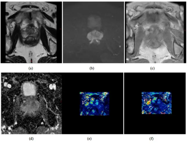
A typical prostate multiparametric MR study includes a morphological T2-weighted (T2-W) series and a functional series, including diffusion weighted imaging (DWI) sequences and perfusion T1-weighted sequences, acquired before, during and after contrast agent administration (also called dynamic contrast enhanced [DCE] MRI). In some cases, these studies also include spectroscopic analysis. For multiparametric analysis, several DWI sequences with different diffusion gradients are acquired and used to compute the apparent diffusion coefficient (ADC) map. The DCE images are used to analyze the tissue enhancement, either visually or using time/intensity curves and semi-quantitative parameters, such as the area under the enhancement curve, wash in and wash out rates and time to peak. Computation of pharmacokinetic parameters can also be used to characterize tissue microcirculation, for example, using Tofts’ model, where Ktransis the transfer constant between the blood plasma and the extra-vascular extra-cellular spaces (EES), Kepis the exchange constant rate between the EES and the blood plasma, and Veis the extra-vascular extra-cellular volume[2;3] (Figure 1).
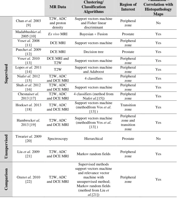
In this context, and because MRI involves an enormous number of data to interpret, many authors have investigated automatic classification algorithms to design MRI-based computer-aided diagnosis (CAD) tools and software for cancer characterization. The current standard paradigm for CAD systems is as a second reader. After the radiologist has evaluated multiple imaging sets, CAD is used to indicate the likelihood that a given suspicious region is malignant. Most of the employed methods are based on supervised classification techniques, in which a set of pre-interpreted patient data must be used as a learning step (Table 1). These approaches have presented two main limitations. First, the performance of the algorithm depends on the quality and volume of the training data. Second, the learning step requires retrospective data, which might be either obsolete or center-specific.
4
Figure 1: Examples of multiparametric magnetic resonance images: (a) T2 weighted sequence, (b) diffusion
weighted images (DWI), (c) T1 weighted dynamic contrast enhance (DCE) images, (d) the apparent diffusion coefficient map computed from the diffusion weighted sequences and (e) and (f) pharmacokinetics parameters computed from the DCE sequences. The transfer constant between the blood plasma and the extra-vascular extra-cellular spaces (Ktrans) and the exchange constant rate between the extra-vascular extra-cellular spaces and
5 MR Data Clustering/ Classification Algorithms Region of Interest Validation – Correlation with Histopathology Maps Su pervi se d Chan et al. 2003 [9] T2W, ADC and proton density
Support vectors machine and Fisher linear
discriminant
Peripheral
zone No Madabhushiet al.
2005 [10] Ex vivo MRI Bayesian + Fusion Prostate Yes Voset al. 2008
[11] DCE MRI Support vectors machine
Peripheral
zone Yes Puechet al. 2009
[12] DCE MRI Decision tree Prostate Yes Voset al. 2010
[13]
DCE MRI and
T2W Support vectors machine
Peripheral
zone Yes Lopes et al. 2011
[14] T2W
Support vectors machine and Adaboost Peripheral zone Yes Niafet al. 2012 [15] T2W, ADC
and DCE MRI 4 classifiers
Peripheral
zone Yes Shah et al. 2012
[16]
T2W, ADC
and DCE MRI Support vectors machine
Peripheral
zone Yes Chesnaiset al.
2013 [17]
T2W, ADC and DCE MRI
4 classifiers (method from Niafet al.[15]) Peripheral zone Yes Hoekset al. 2013 [18] T2W, ADC and DCE MRI
Support vectors machine (methodfrom Vos et al.
[13] ) Transition zone Yes Hambrocket al. 2013 [19] T2W, ADC and DCE MRI
Support vectors machine (methodfrom Vos et al.
[13] ) Peripheral zone and transition zone Yes U nsupervi se d Tiwariet al. 2009
[20] Spectroscopy Hierarchical Prostate No
Liu et al. 2009 [21]
T2W, ADC
and DCE MRI Markov random fields
Peripheral zone Yes C om par ison Ozeret al. 2010 [22] T2W, ADC and DCE MRI
Supervised methods support vectors machine
and relevance vector machine with unsupervised method; Markov random fields (method from Liu et
al.[21])
Peripheral
zone Yes
Table 1: State of the art of classification and clustering methods applied for prostate magnetic resonance image
analysis. The methods are grouped into two categories: supervised and unsupervised. Classification is also performed according to the criteria for the MR images sequences used: T2-weighted (T2W), dynamic contrast enhanced (DCE), apparent diffusion coefficient (ADC) computed from the diffusion weighted (DW) sequences and spectroscopy images, as well as the proton density sequence. The clustering technique used, region of interest (entire gland or specific area, such as the peripheral zone) and the validation with the ground truth from the histopathological maps are also indicated.
6
In this study, we began with the assumption that a multiparametric approach would be optimal for all of the images. We then proposed an unsupervised method for prostate tissue classification from multiparametric MR images. This method was not designed for the detection of cancer or suspicious lesions but rather was intended to be used as an analysis tool, allowing us to merge information from all available sources to address conflict and redundancy and to provide a unique homogeneous pattern (tissues) map.
We investigated the use of evidence theory. This approach, also known as belief functions theory, is becoming widely used in multisource data analysis. It provides an advanced modeling of fusion, conflicts among sources and outliers[4]. Several applications of this reasoning in medical image analysis and CAD can be found (e.g., in brain MRI segmentation and tumor detection)[5;6].Our proposed approach is an adaptation of the evidential C-means classifier (ECM) introduced by Masson and Denoeux[7]. We successfully applied this method to multiparametric prostate MR data in a previous work, in which the aim was to segment and separate the prostate into two compartments: peripheral and transition zones[8].
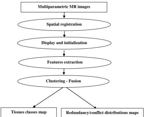
2. Methods
Figure 2 depicts the pipeline of the method.Figure 2: The pipeline of the method. The multiparametric data are first spatially registered. After feature
extraction, evidential theory-based clustering is used to reduce the data into homogeneous classes.
Multiparametric MR images
Spatial registration
Clustering - Fusion Features extraction
Redundancy/conflict distributions maps Display and initialization
7
2.1 Data preparation: spatial registration and feature extraction
The multiparametric MR sequences could not be processed directly for two reasons. First, most of the images were acquired from different fields of view and thus had different spatial resolutions. Second, there were patient movements between acquisitions. Therefore, the first step was spatial registration and normalization. Because T2W images are regarded as the cornerstone for prostate morphology evaluation, these images were considered the reference space, and the other sequences were strictly registered to this space using standard affine registration algorithms based on maximization of mutual information. Following this spatial matching, resampling and interpolation were used to match the other sequences with the T2W images in terms of resolution.
After this pre-processing, each prostate voxel was described by a feature vector containing the image features as gray levels from the T2W images, the ADC and the pharmacokinetic parameters (Ktrans, Kep and Ve).
A previous study [23] demonstrated that the local parameters, computed using fractal geometry, allowed for better detection of heterogeneities in prostate tissues from T2W MR images than from the native gray level values. Fractal geometry is a powerful tool for texture analysis that can be used to process medical imaging data efficiently. The fractal geometry can be measured using the fractal dimensions (FDs). We computed the local 3D FDs for each 7x7x3 region of interest (ROI) using the Variance method [24]. Thus, instead of considering the T2W image gray levels, a local fractal dimension was estimated for each voxel.
By combing all of the MR data, a features set including the local fractal dimension, the ADC value and the pharmacokinetic parameters Ktrans, Ve the was associated to each voxel as follows:
Voxel (Vi) = FD, ADC, Ktrans , Ve (1) After processing, the data were normalized and standardized for the range of different features. For each feature, the mean and the standard deviation were computed. For each feature value, the mean was then subtracted, and the result was divided by the standard deviation.
8 2.2 Source modeling and clustering
a. Initialization
Our method was designed to assist radiologists in analyzing large numbers of images by fusing the sources into a single map. The voxels were described by their features (equation 1) and were grouped into homogeneous patterns. Class initialization is a key step in any clustering process for addressing this issue. Our proposed approach was inspired by radiologists’ behavior when cognitively analyzing MR images. Generally, the most sensitive images, typically pharmacokinetic and ADC images are analyzed first to detect and highlight the suspicious regions. To refine the analysis, several cross-analyses are performed using all of the image sequences.
In this regard, the Ktrans map could be used to define the initial classes map. First, the image histogram was constructed, and a mode recognition algorithm[25] was applied to detect the class number. Then, the K-means algorithm was used for clustering. The results were applied to the remaining image sources to obtain the configuration of the first classes.
b. Evidential modeling
Evidential reasoning associates a data source or sensor, S, with a set of propositions, also known as the ―frame of discernment‖. In a classification context, the frame of discernment, denoted as , is the set of classes. If 𝜔1, . . , 𝜔𝑘 denote these classes, then= ω1, . . , ωk Let P = P1, … , PN be the set of patterns/objects to be assigned to one of theclasses. Evidential reasoning allows for the extraction of the partial knowledge of this assignment, called the ―basic belief assignment‖ (bba). A bba is a function that takes values in the range 0, 1and defines the 2subsets of ( ∅, ω
1, . . , ωk, ω1∪ ω2, . . , ). For each pattern 𝑃𝑖 ∈ 𝑃, a
bba(denoted as 𝑚𝑖) allows us to measure the assignment to each subset A of such that the
following relationship is true:
mi(A) = 1 A
(2)
The higher the value of 𝑚𝑖 𝐴 is, the stronger the belief for assigning 𝑃𝑖 to A. For instance, 𝑚𝑖 𝜔𝑗 = 1 implies that ∀𝐴 ⊆ 𝛺, 𝐴 ≠ 𝜔𝑗 , 𝑚𝑖 𝐴 = 0. This means that 𝑃𝑖 is assigned to 𝜔𝑗 . However, if 𝑚𝑖 𝜔𝑗 = 0.5 , 𝑚𝑖 𝜔𝑙 = 0.2 and 𝑚𝑖 𝜔𝑗, 𝜔𝑙 = 0.3 , there is a stronger belief for assigning 𝑃𝑖 to 𝜔𝑗 than to 𝜔𝑙 . It also highlights that there is a 20%
9
belief for assigning 𝑃𝑖 to the union of the 2 classes, which can be interpreted as a doubt regarding pattern membership. In contrast to the fuzzy sets model, evidential reasoning can extend the partial membership concept by assigning beliefs not only to classes but also to unions of classes. This feature is particularly useful in cases in which the classes overlap. Using this model, Denoeux and Masson [26] introduced a new type of data partition called the ―credal partition‖. This partition can be seen as an extension of the fuzzy partition, with bba functions replacing the fuzzy membership functions. The authors later proposed an evidential version of the C-means classifier (the ECM) that used a credal partition, which was inspired by the fuzzy C-means (FCM) algorithm [7]. This algorithm classifies N patterns into k classes of , based on the class centers and the minimization of a cost function. As is the case for fuzzy partitions in FCM, the credal partition (in which each line is a bba𝑚𝑖 associated with a pattern 𝑃𝑖) is optimized iteratively. Further details on this generic classification method can be found in [7].
c. Spatial relaxation
The ECM model, as previously described, extracts and optimizes partial knowledge for pattern assignments. The ECM model can be used to classify voxels directly as independent data objects. However, the voxel neighborhoods, defined by the connexity system, provide valuable information. In fact, the image segmentation supposes that the image regions share common features. Connexity and neighborhood systems model this assumption using region-oriented segmentation methods, such as growing regions or hidden Markov field models. In a homogeneous region or class, a bba not only provides information on a pattern but also on its connected neighbors. Corrupted information, extracted from outliers/noise patterns, can be relaxed using the information from neighbors. Thus, introducing neighborhood information in ECM modeling can provide the following advantages:
• Modeling of contextual region information by extracting information from the patterns/voxels;
• Reduced corrupted information related to outliers and noise; and
• Assimilation of the ECM classifiers into region-based segmentation processes.
The bbami of pattern Pi (associated with voxel Vi) was relaxed by combining it with
bbafunctions from spatially connected neighbors. Spatial connection was defined by a 3D
10
bbacombination operator [27].
Let 𝑚𝑖 be the bba of the pattern 𝑃𝑖 and 𝑚𝑖1, ⋯ , 𝑚𝑖26 be the bba functions from 𝑃𝑖’s 26 connected neighbors 𝑃𝑖1, ⋯ , 𝑃𝑖26 . We denote as 𝑚𝑖′, the result of combining 𝑚𝑖 and 𝑚𝑖1, ⋯ , 𝑚𝑖26 ∀ A 𝑚𝑖′ A = 𝑚𝑖 A1 ⋯ 𝑚𝑖26 Af A1∩⋯∩Af=A A1⋯Af⊆Ω (3)
However, the contribution of each neighbor to this combination should be weighted by its distance from the considered voxel. This combination is particularly relevant for prostate MRI, in which the voxels are significantly anisotropic. Based on this reasoning, the neighboring
bbafunctions were weighted as follows.
Let 𝑚𝑖𝑗𝑗 be the result of weighting 𝑚
𝑖𝑗 ∀ A 𝑚𝑖𝑗𝑗 𝐴 = 𝑗. 𝑚𝑖𝑗(𝐴) 𝑚𝑖𝑗𝑗 = 1 − 𝑗 + 𝑗. 𝑚𝑖𝑗() Where (4) αj = γ dij2 (5)
0 ≤ 𝛾 ≤ 1is a parameter, and dij is a normalized Euclidean distance between voxel 𝑣𝑖 and its
spatial neighbor 𝑣𝑖𝑗. Using equation (3) and replacing the neighboring bba functions with the weighted ones (4), we define 𝑚𝑖′as follows.
∀ A
𝑚𝑖′ A = 𝑚𝑖 A1 . 𝑚𝑖11 A2 ⋯ 𝑚𝑖2626 Af A1∩⋯∩Af=A
A1⋯Af⊆Ω
(6)
This combination is used as a relaxation step that allows for correction of the evidential assignment of a voxel based on the information from its neighbors.
11 2.3 Decision-making
At the level of bbafunction extraction and optimization, we measure belief for the membership of each voxel to one of the classes𝜔 ∈. However, we also measure belief for the empty set and subsets 𝐴, which could be interpreted as ―doubt‖ regarding the membership of the voxel. A decision still must be made to classify the voxels into one of the classes. This decision is reached by transforming the bba 𝑚𝑖 into a probability measurement, as calculated by ∀ωi ∈ Prob ωi =1 − 𝑚1 𝑖() 𝑚𝑖(A) A ωA A⊆Ω (7)
where 𝐴 denotes the number of elements in A and is the empty set.
Finally, we define the decision rule R that associates the pattern 𝑃𝑖 with one of the classes of as follows.
R 𝑃𝑖 = argmax
ω ∈ Prob ωi
(8)
2.4 Results presentation
For the presentation of the results, two levels are proposed. The first level displaysa single 3D class map with a color associated with each class. This map labels all of the voxels with one of the 𝜔1, . . , 𝜔𝑘 classes. It also renders the tissue distribution homogeneous. For interpretation purposes, the map can be merged with any of the original image sources.
The second display level provides a more detailed description of the clustering results. The different probability maps resulting from the belief membership conversion (equation 7) are displayed using color maps. These maps could be very useful in addressing conflict regions. Indeed, they include the empty set probabilistic distribution. The empty set is associated with the reject class, grouping all of the voxels that could not be clearly associated with one of the classes (i.e., the probability of the empty set was the greatest).
The maps also include all of the other subset cases.
For instance, for a typical case with 2 classes, 𝜔1 =healthy tissue and 𝜔2 =suspicious tissue, the clustering produced 4 maps: a probability map for each class and a probability map for the 2 class unions in which a voxel has the same probability of being in either class. The last map
12 is the empty set map, which groups the outliers.
The first level display creates the homogeneous tissue map by combining the 2 results of classes 𝜔1and 𝜔2.
3. Experiments and Results
In this section, we report the results of the method applied to synthetic data with a known ground truth for class distribution and clinical images correlated with histopathology findings. 3.1 Simulated image experiments
The aims of these experiments were to test and evaluate the clustering process with regard to noise.
a. Creation
Simulation of multiparametric MR images is a difficult process. Moreover, a complete simulation should model and simulate the tumor behavior for all of the MR sequences (T2W, DCE, DWI and spectroscopy). To our knowledge, these behaviors are not yet well known. Nevertheless, to highlight the performance of the ECM clustering combined with spatial neighboring relaxation on multi-source data, we rendered multi-parametric images using 3 MR clinical sequences: T2W, DCE and DWI. For each sequence, a radiologist delineated the peripheral and transition zones. The transition zone (TZ) was then filled with its mean value. The peripheral zone (PZ) level was deduced using a pre-determined contrast value C defined as
C = ITZ − IPZ ITZ + IPZ
(9)
whereITZand IPZ are the mean MR signals of TZ and PZ in the considered sequence, respectively.
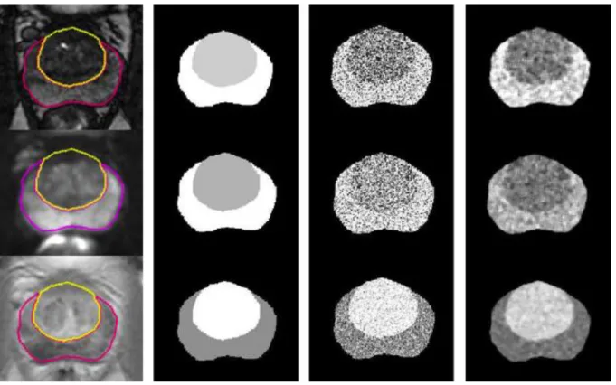
Gaussian noise was added, and a median filter was applied to reduce the salt-pepper aspect of the noisy images so that they would be more similar to the real data. Figure 3 illustrates this process.
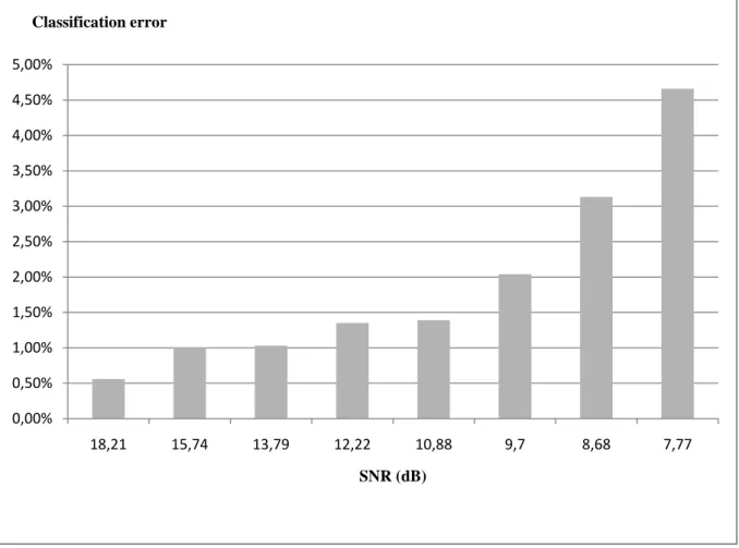
13 SNRdb = 10log I0 2 i=1..n I − I0 2 i=1..n (10)
where I0 and I are the intensities before and after adding the Gaussian noise, respectively. Finally, the rendered images had different quality levels. The signal-to-noise ratios ranged from 18.21 dB to 7.77 dB, and the contrast levels (C, equation 9) ranged from 0.1 to 0.25.
Figure 3: The image simulation process. From left to right: original MRI with pre-delineated peripheral and
transition zones, the zones labeled with their respective mean level, data with Gaussian noise and data after a smoothing median filter. The first, second and third lines represent the T2W, DWI and DCE images, respectively.
b. Results
The evaluation of the classification method for the synthetic data consisted of the accurate segmentation of the peripheral and transition zones. The evaluation was performed using the classification error from the voxel labeling.
14
Figure 4: The results expressed as classification errors for labeling voxels belonging to either the peripheral or
transition zones from multi-source data with different noise levels.
3.2 Real data evaluation a. Description
For clinical evaluation, we considered the abilities of the method to segment cancerous regions. For this purpose, a retrospective study was done. Multiparametric MR images were collected from 15 patients. The data consisted of T2W images with a 0.48×0.48×4.00 mm3 voxel size (15 slices by volume), T1W DCE MRI images with a 0.61×0.61×4.00 mm3 voxel size (15 slices by volume, 20 dynamics) and an ADC map computed from 2 DWI acquisitions using b=0 and b=600 with a 1.12×1.12×4.00 mm3 voxel size (15 slices by volume). The DCE images were processed in-house using software implementing Tofts’ model to generate the pharmacokinetic Ktrans, Ve, and Kepmaps.
As described above, the MR volumes were registered and interpolated to fit the T2W resolution.
All of the patients underwent radical prostatectomy. To have a true diagnosis, the histological findings were correlated with MRI data. The prostate specimens were stained, fixed and
0,00% 0,50% 1,00% 1,50% 2,00% 2,50% 3,00% 3,50% 4,00% 4,50% 5,00% 18,21 15,74 13,79 12,22 10,88 9,7 8,68 7,77 Classification error SNR (dB)
15
sectioned according to the Stanford protocol[28] (Figure 5-a). A reconstructed histological map of each prostate was created (Figure 5-b). The contours of the histological zones, as well as the outlines of each cancer, were drawn on the slides under a microscope. The results from these analyses were reported on the MR images by manual correspondence with the histology images. This task was performed by experienceduro-radiologists, according to the method described in [29]. The prostate was divided into eight regions of interest by the octant technique. The top and bottom were divided into four quadrants, corresponding to the transition zone (TZ) and peripheral zone (PZ) on the left and right. Within each octant, the TZ, PZ and anterior fibromuscular stromal boundaries were traced. The tumor was located according to these histological zone boundaries.
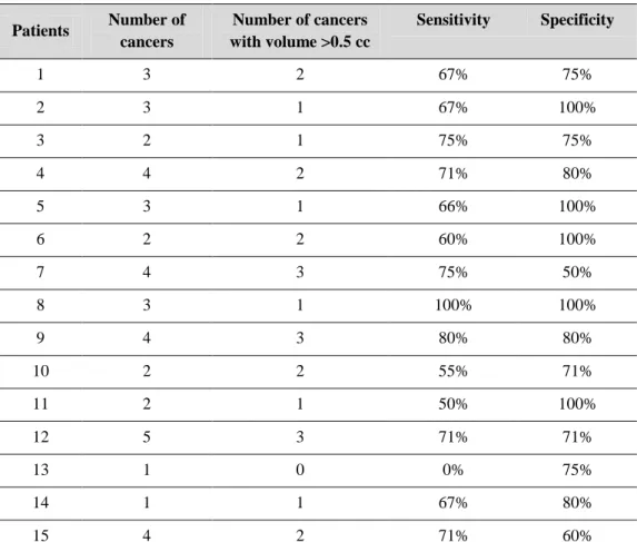
Out of 15 patients, a total of 43 tumors were considered, including 25 tumors with a volume greater than 0.5 cc (Table 2).
Figure 5: (a) Histopathology image. (b) Cancer maps created from the histopathology images.
b. Results
For quantitative evaluation, we measured the ability of the method to distinguish tumor patterns from healthy tissue patterns. For this purpose, at the end of the clustering process, the resulting 3D map was merged with the anatomical T2W MR images, allowing the radiologist to label and associate the different classes to the tissue classes (peripheral zone, transition zone, etc.) and thus isolate the suspicious regions (tumors). By comparing the results to the
16
actual diagnosis for each patient, the numbers of truepositives, falsepositives, truenegatives and falsenegatives could be evaluated for different regions of interest. Sensitivity and specificity were computed, respectively, as follows.
sensitivity = true positives
true positives + false negatives specificity = true negatives
true negatives + false positives
Patients Number of cancers Number of cancers with volume >0.5 cc Sensitivity Specificity 1 3 2 67% 75% 2 3 1 67% 100% 3 2 1 75% 75% 4 4 2 71% 80% 5 3 1 66% 100% 6 2 2 60% 100% 7 4 3 75% 50% 8 3 1 100% 100% 9 4 3 80% 80% 10 2 2 55% 71% 11 2 1 50% 100% 12 5 3 71% 71% 13 1 0 0% 75% 14 1 1 67% 80% 15 4 2 71% 60%
Table 2: Histopathologic analysis of the 15 patients included in the study and the results obtained using the
proposed fusion method.
The mean sensitivity and specificity were 65% (0%-100%) and 81% (50%-100%), respectively. The worst scores corresponded to tumors with volumes less than 0.5 cc. This value is currently accepted as a limit for tumor detection on MR imaging. By considering only tumors with volumes greater than the 0.5 cc threshold, the mean sensitivity and specificity grew to 70% and 88%, respectively.
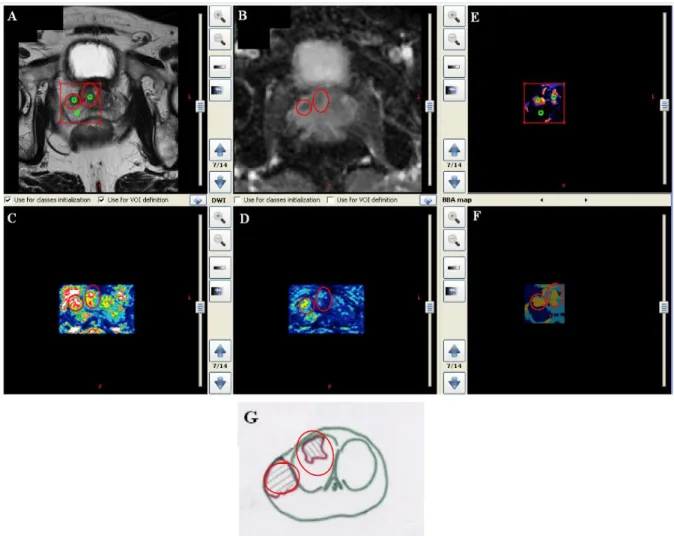
Figure 6 shows a case in which 3 classes were detected. The result (Figure 6-F) depicts the class map, which highlights a class for the peripheral zone, a class for the transition zone
17
tissue and a third class composed of data from 2 patterns that could be interpreted as a tumor. Returning to the MR images, one of these patterns was clearly depicted in the 4 images (T2W, ADC, Ktransand Ve), while the second was only visible as a hyper-vascular area on the Ktransmap. The fusion allowed us to place these two patterns in the same class. The ground truth image (G) revealed two tumors (circles).
Figure 6: Classification results – Example 1. (A) T2W image with the region of interest to be analyzed. Three
tissues are defined: part of the PZ, part of the TZ and a suspected area. (B) The ADC map. (C) The Ktrans map.
(D) The Ve map. (F) Fusion map showing the distribution of the 3 tissues. (E) Basic belief assignment (bba) map
showing the membership degree of each voxel to the 3 classes. (G) The ground truth.
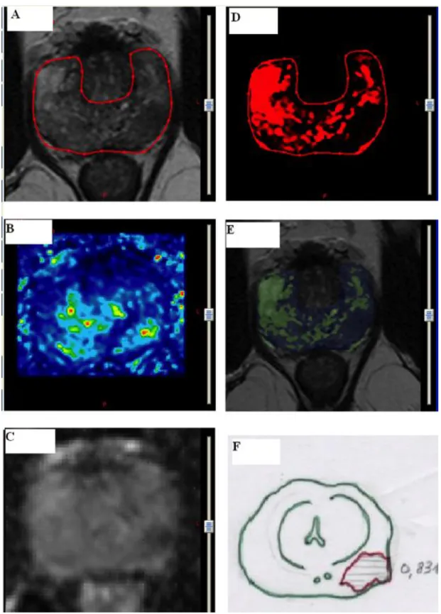
Figure 7 depicts a case in which the analysis focused only on the peripheral zone, using 3 sources: the T2W (Figure 7-A), the Ktrans(Figure 7-B) and the ADC (Figure 7-C) maps. Initialization was performed starting with the ADC map. The result of the fusion (Figure 7-E) is displayed in the superposition mode for the T2W image, whereas Figure 7-D shows the bba map. Both maps (D and E) highlight a region corresponding to the optimal fusion among the hypo-signal of the ADC map, the hyper-signal of the Ktrans and the T2W hypo-signal. Figure
18 7-F shows the ground truth.
Table 2 summariesthe histopathology data for the 15 patients and the results quantified using the sensitivity and specificity.
Figure 7: Classification results – Example 2. (A) T2W image with peripheral zone delineation. (B) The Ktrans
map. (C) The ADC map. (D) The basic belief map. (F) The fusion map of images A, B and C. The result is merged with the T2W (A) image. (F) The ground truth.
19
4. Discussion - Conclusion
In this study, we described an unsupervised fusion scheme to analyze multiparametric MR images. This proposed framework was not designed for cancer detection or characterization but rather as a tool to assist radiologists in analyzing multi-source data. Because it is fully automatic, it can be applied in clinical routines for preliminary analysis and to fuse multiple MR sequences into a single 3D map in which the voxels that exhibit similar behaviors in all of the sequences are grouped into classes.
The method is based on a spatial registration and a normalization step that standardizes the data, followed by a multi-source clustering step that is driven by the evidential c-means algorithm. A relaxation step is introduced in this algorithm to integrate the voxel spatial neighborhood information. As a result of this relaxation, the basic belief for the assignment of each voxel can be corrected using information from connected neighbors, via a conjunctive combination of the bbafunctions.
The combination of the ECM algorithm with this spatial relaxation allowed us to perform clustering and segmentation on simulated multi-source data with different noise levels (Figure 3), with accuracy of 95% (Figure 4).
Two-level result reporting was proposed. The first level used a single map that represented homogeneous tissue distribution, while the second level was a membership degrees image. This image maps the source conflict regions.
We validated our method by analyzing clinical data from 15 patients. The method had mean sensitivity and specificity of 65% and 81%, respectively. These tests considered data consisting of grouped tumors, with different volumes from both the peripheral zone and the transition zone.
To our knowledge, there has been only one previously published study, by Liu et al.[21], in which the authors used an unsupervised classification method to diagnose prostate cancer using multiparametric MR images. The method was based on fuzzy Markov random fields, in which the parameters were implicitly estimated and combined with the segmentation process. However, the previous method was parametric because Gaussian distributions were assumed for the classes. Our approach was free from any assumptions regarding class distributions. Compared with the previously reported methods, which have mainly been based on supervised classification algorithms, our results might appear weak. Indeed, the supervised
20
techniques described in Table 1 reported sensitivity and specificity scores of at least 85%. However, as discussed in the Introduction section, supervised classification requires an extensive learning process, and the most important issue with this type of approach is that the learning step must be updated each time the data change due to changes in the acquisition protocol.
In a study by Ozeret al.[22], two supervised methods were compared with an unsupervised algorithm (Liu et al. [21]). It was concluded that the supervised algorithms performed better than the unsupervised algorithm. In general, when the data are similar to those used during the learning process, in which all of the classification parameters are optimized, supervised approaches outperform unsupervised approaches. This situation changes if new data are used. In clinical practice, such a change often occurs due to changes in the acquisition protocols, when new MR sequences parameters or new machine are used.
Without the inclusion of any learning or calibration steps, the preliminary results for our unsupervised approach to computer-aided analysis of multiparametric MR images showed promising results. Moreover, the global framework described here could be extended to other multimodality sources. Indeed, photon emission tomography (PET) has the ability to analyze quantitative biomarkers that assess a host of physiological and biochemical tumor characteristics. Ultrasound elastography could also be valuable for tissue characterization. The only limitation for the integration of all of these sources into the proposed approach is spatial registration.
The fusion strategy employed in this study attributed equally distributed confidence levels to the different image sources. However, specific parameterization using different weights is also possible. Tiwariet al. [30] investigated the weighted combination of multiparametric MR imaging for the evaluation of radiation therapy outcomes, and they reported promising results. The weighted combination of multiparametric or multimodality sources provided specific confidence levels for each imaging modality, according to its sensitivity and specificity. This combination could easily be applied for basic belief assignment modeling. It could also be used at different stages during initialization or before final fusion and conversion of the
bbafunctions into class membership degrees.
Another important issue concerns validation. The evaluation described here was a single-observer study. Currently, we are preparing a more extensive evaluation with a more relevant patient base and better selection criteria, such as limitation to only one zone (peripheral or
21
transition zones) and consideration of only clinically significant tumors larger than the threshold of 0.5 cc. This evaluation will be a multi-observer study.
Lastly, it is understood that the proposed approach will not replace supervised approaches. As clearly indicated, our method is not a diagnostic technique. The development and implementation of supervised techniques for distinguishing aggressive tumors from benign lesions remain of great importance to clinical practice.
Conflict of interest
Nacim Betrouni, Nasr Makni, Said Lakroum, Philippe Puech, ArnauldVillers and Serge Mordon declare that they have no conflict of interest.
Informed Consent
22 References
[1] Tanimoto A, Nakashima J Kohno H Shinmoto H Kuribayashi S. Prostate cancer screening: the clinical value of diffusion-weighted imaging and dynamic MR imaging in combination with T2-weighted imaging. J MagnReson Imaging 25 (1):146-152, 2007.
[2] Tofts, P. S., Berkowitz, B., and Schnall, M. D.Quantitative analysis of dynamic Gd-DTPA enhancement in breast tumors using a permeability model –MagnReson Med 33 (4), 1995.
[3] Quantitative Imaging Biomarkers Alliance.DCE MRI Quantification profile, http://rsna.org/QIBA_.aspx 2012.
[4] Bloch I. Some aspects of dempster-shafer evidence theory for classification of multi-modality medical images taking partial volume effect into account. Pattern Recognition Letters 17 (8):905-920, 1996 [5] Capelle, A.S. Colot O., Fernandez-Maloigne C.Evidential segmentation scheme of multi-echo MR images
for the detection of brain tumors using neighborhood information. Information Fusion 5 (3):203-216, 2004
[6] Chen, S.Y. J., Lin, W. C., and Chen, C. T.Evidential reasoning based on Dempster-Shafer theory and its application to medical image analysis. Neural and Stochastic Methods in Image and Signal Processing II 2032:35-46, 1993
[7] Masson, M.H Denoeux T.ECM: An evidential version of the fuzzy c-means algorithm. Pattern Recognition 41:1384-1397, 2011
[8] Makni N, IancuA, Colot O, Puech P, Mordon S, Betrouni N. Med Phys.Zonal segmentation of prostate using multispectral magnetic resonance images. Medical Physics 38 (11):6093-6105, 2011
[9] Chan, W. Wells R., Mulkern S., Haker J., Zhang K. Zou S. Maier and C. Tempany.Detection of prostate cancer by integration of line-scan diffusion, t2-mapping and t2-weighted magnetic resonance imaging: a multichannel statistical classifier. Medical Physics 30 (9):2390-2398, 2003
[10] Madabhushi M., Feldman D., Metaxas J., Tomaszeweski and D. Chute. Automated detection of prostatic adecarcinoma from high-resolution ex vivo MRI. IEEE Transactions on Medical Imaging 24 (12):1611-1625, 2005
[11] Vos P.C, T. Hambrock, C. A. Hulsbergen-van de Kaa J. J. Fü and tterer, J. O. Barentsz and H. J. Huisman.Computerized analysis of prostate lesions in the peripheral zone using dynamic contrast enhanced MRI. Medical Physics 35 (3):888-899, 2008
[12] Puech P, N. Betrouni N., Makni, A.S. Dewalle, A. Villers and L. Lemaitre.Computer-assisted diagnosis of prostate cancer using DCE-MRI data: design, implementation and preliminary results. International Journal of ComputerAssisted Radiology and Surgery 4:1-10, 2009
[13] Vos P.C., T. Hambrock J. O. Barenstz and H. J. Huisman.Computer-assisted analysis of peripheral zone prostate lesions using t2-weighted and dynamic contrast enhanced t1-weighted MRI. Physics in Medicine and Biology 55 (6):1719, 2010
[14] Lopes R., A. Ayache, N. Makni, P. Puech, A. Villers, S. Mordon, N. Betrouni.Prostate cancer characterization on MR images using fractal features. Medical Physics 38 (1):83-95 2011
[15] Niaf E, Rouvière O, Mège-Lechevallier F, Bratan F, Lartizien C.Computer-aided diagnosis of prostate cancer in the peripheral zone using multiparametric MRI. Physics in Medicine and Biology 57 (12):3833-3851, 2012
[16] Shah V, Turkbey B Mani H Pang Y Pohida T Merino M Pinto PA Choyke PL Bernardo M. Decision support system for localizing prostate cancer based on multiparametric magnetic resonance imaging. Medical Physics 39 (7):4093-4103, 2012
[17] Chesnais AL, Niaf E, Bratan F, Mège-Lechevallier F, Roche S, Rabilloud M, Colombel M Rouvière O.Differentiation of transitional zone prostate cancer from benign hyperplasia nodules: evaluation of discriminant criteria at multiparametric MRI. Clinical Radiology 68 (6):323-330, 2013
[18] Hoeks CMA, Hambrock T, Yakar D, Hulsbergen-van de kaa CA, Feuth T, Witjes JA, Fütterer JJ, Barentsz JO. Transition Zone Prostate Cancer: Detection and Localization with 3-T Multiparametric MR Imaging. Radiology 266:207-217, 2013.
[19] Hambrock T, Vos PC, Hulbergen-van de Kaa CA, Barentsz JO, Huisman HJ. Prostate Cancer: Computer-aided Diagnosis with Multiparametric 3-T MR Imaging—Effect on Observer Performance. Radiology 266 (521): 530, 2013.
23
[20] P.Tiwari, M. Rosen and A. Madabhushi.A hierarchical spectral clustering and nonlinear dimensionality reduction scheme for detection of prostate cancer from magnetic resonance spectroscopy (mrs). Medical Physics 39 (9):3927-3939, 2009
[21] X.Liu, D. L. Langer, M. A. Haider, Y. Yang, M. N. Wernick and Yetik.Prostate cancer segmentation with simultaneous estimation of markov random field parameters and class. IEEE Transactions on Medical Imaging 28 (6):906-91, 2009
[22] Ozer S, Langer D Liu X. Haider M. van der Kwast T. Evans A. Yang Y. Wernick M. Yetik I.Supervised and unsupervised methods for prostate cancer segmentation with multispectral MRI. Medical Physics 37 (4):1873-1883, 2010.
[23] Lopes R., AyacheA, Makni N. Puech P Villers A. Mordon S. Betrouni N.Prostate Cancer characterization on MR images using fractal features. Medical Physics 38 (1):83-95, 2011.
[24] Lopes R. and Betrouni N. Fractal and multifractal analysis: A review Medical Image Analysis, Medical Image Analysis, 13 (4), 634-649, 2009.
[25] Postaire JG and Vasseur C. An approximate solution to normal mixture identification with application to unsupervised pattern classification. IEEE Trans Pattern Anal Mach Intell 3 (2):163-179, 1981
[26] Denoeux, T and Masson M. H. Evidential clustering of proximity data.IEEE Transactions on Systems, Man and Cybernetics.34:95-109 2004.
[27] Smets P.Analyzing the combination of conflicting belief functions - Information Fusion 8(4):387-412, 2007
[28] J.E.McNeal and O.Haillot. Patterns of spread of adenocarcinoma in the prostate as related to cancer volume.Prostate 49:48-57, 2001.
[29] Puech P., Potiron E. Lemaitre L. Leroy X. Haber GP Crouzet S. Kamoi K Villers A.Dynamic Contrast-enhanced-magnetic Resonance Imaging Evaluation of intraprostatic Prostate Cancer: Correlation with Radical Prostatectomy Specimens. Urology 74 (5):1094-1099, 2009
[30] Tiwari P., Viswanath S. Kurhanewicz J. Madabhushi A.Weighted combination of multi-parametric MR imaging markers for evaluating radiation therapy related changes in the prostate 80-91, 11, Berlin - Heidelberg