Distributed inference : combining variational inference with distributed computing

Combining Variational

Inference With Distributed Computing

by

Chris Calabrese

S.B. Computer Science and Engineering,

Massachusetts Institute of Technology, 2011

Submitted to the

ARC6

W

;e H/E F

jj9

Department of Electrical Engineering and Computer Science

in partial fulfillment of the requirements for the degree of

Master of Engineering in Electrical Engineering and Computer Science

at the

MASSACHUSETTS INSTITUTE OF TECHNOLOGY

February 2013

Massachusetts Institute of Technology 2013. All rights reserved.

A u th o r ...

Chris Calabrese

Department of Electrical Engineering and Computer Science

/If

Certified by

U

February 5, 2013

David Wingate

Research Scientist

Thesis Supervisor

Accepted by...

Prof. Dennis M. Freeman

Chairman, Masters of Engineering Thesis Committee

Distributed Inference: Combining Variational Inference

With Distributed Computing

by

Chris Calabrese

Submitted to the Department of Electrical Engineering and Computer Science on February 5, 2013, in partial fulfillment of the

requirements for the degree of

Master of Engineering in Electrical Engineering and Computer Science

Abstract

The study of inference techniques and their use for solving complicated models has taken off in recent years, but as the models we attempt to solve become more complex, there is a worry that our inference techniques will be unable to produce results. Many problems are difficult to solve using current approaches because it takes too long for our implementations to converge on useful values. While coming up with more efficient inference algorithms may be the answer, we believe that an alternative approach to solving this complicated problem involves leveraging the computation power of multiple processors or machines with existing inference algorithms. This thesis describes the design and implementation of such a system by combining a variational inference implementation (Variational Message Passing) with a high-level distributed framework (Graphlab) and demonstrates that inference is performed faster on a few large graphical models when using this system.

Thesis Supervisor: David Wingate Title: Research Scientist

Acknowledgments

I would like to thank my thesis advisor, David Wingate, for helping me work through this project and dealing with my problems ranging from complaints about Matlab to my difficulties working with some of the mathematical concepts in the study of inference. Most importantly, his efforts helped me develop some kind of intuition for the subject matter relevant to this project, and that is something I know I can use and apply in the future.

Contents

1 Introduction

1.1 Example: Inference on Seismic Data . . . .

1.2 Variational Message Passing and Graphlab . . .

1.2.1 Variational Inference and VMP . . . . . 1.2.2 Distributed Computation and Graphlab

1.3 Contributions . . . . 2 Variational Message Passing

2.1 Bayesian Inference . . . .

2.1.1 Example: Fair or Unfair Coin? . 2.2 Variational Inference . . . .

2.3 Variational Message Passing . . . .

2.3.1 Message Construction . . . . . 2.3.2 Operation Details . . . .

3 Graphlab Distributed Framework 3.1 Parallel/Distributed Computation . . .

3.1.1 Parallel Computing . . . .

3.1.2 Distributed Computing . . . . .

3.2 Parallel/Distributed Frameworks . . . 3.2.1 Distributed VMP Framework . 3.3 Graphlab Distributed Framework . . . 3.3.1 Graphlab PageRank Example .

11 12 14 14 15 16 17 . . . . 17 . . . . 18 . . . . 21 . . . . 23 . . . . 24 . . . . 25 29 . . . . 29 . . . . 30 . . . . 32 . . . . 34 . . . . 35 . . . . 37 . . . . 4 1

4 VMP/Graphlab Implementation Details 49

4.1 VMP Library ... ... 51

4.1.1 Supported Models ... . 57

4.2 VMP/Graphlab Integration ... 61

4.2.1 Creating The Factor Graph ... ... 62

4.2.2 Creating The Vertex Program . . . . 63

4.2.3 Scheduling Vertices For Execution . . . . 65

4.3 Graphical Model Parser . . . . 67

4.4 Current Limitations . . . . 68

5 Results 71 5.1 Parallel Test Results . . . ... . . . . 71

5.2 Distributed Test Results . . . .. . . . . 76

6 Conclusion 81 A Coin Example: Church Code 83 B VMP Message Derivations 85 B.1 Gaussian-Gamma Models . . . . 86

List of Figures

1-1 Complicated inference example: Seismic data [11] . . . . 13

2-1 Results from performing inference on the fairness of a coin. Observed Data = 3H, 2T; Fairness Prior = 0.999 . . . . 19

2-2 Results from performing inference on the fairness of a coin. Observed Data = 5H; Fairness Prior = 0.999 . . . . 20

2-3 Results from performing inference on the fairness of a coin. Observed Data = 5H; Fairness Prior = 0.500 . . . . 20

2-4 Results from performing inference on the fairness of a coin. Observed Data = 10H; Fairness Prior = 0.999 . . . . 20

2-5 Results from performing inference on the fairness of a coin. Observed Data = 15H; Fairness Prior = 0.999 . . . . 20

2-6 Variational Inference: High-Level Diagram . . . . 21

2-7 VMP Example: Gaussian-Gamma Model . . . . 27

3-1 Typical Parallel Computing Environment [28] . . . . 30

3-2 Typical Distributed Computing Environment [28] . . . . 33

3-3 Graphlab: Factor Graph Example [33] . . . . 38

3-4 Graphlab: Consistency Models [33] . . . . 40

3-5 Graphlab: Relationship Between Consistency and Parallelism [33] . . 41

4-1 VMP/Graphlab System Block Diagram . . . . 49

4-2 Supported Models: Gaussian-Gamma Model . . . . 57

4-4 Supported Models: Gaussian Mixture Model [27] . . .

4-5 Supported Models: Categorical Mixture Model [27] . .

Parallel VMP Execution Time: Mixture Components Parallel VMP Execution Time: Observed Data Nodes Parallel VMP Execution Time: Iterations . . . . Distributed VMP Execution: Real Time . . . . Distributed VMP Execution: User Time . . . . Distributed VMP Execution: System Time . . . . B-i VMP Message Derivations: Gaussian-Gamma Model . B-2 VMP Message Derivations: Dirichlet-Categorical Model 5-1 5-2 5-3 5-4 5-5 5-6 58 59 . . . . . 72 . . . . . 74 . . . . . 75 . . . . . 78 . . . . . 79 . . . . . 79 86 90

Chapter 1

Introduction

The ideas associated with probability and statistics are currently helping Artificial Intelligence researchers solve all kinds of important problems. Many modern ap-proaches to solving these problems involve techniques grounded in probability and statistics knowledge. One such technique that focuses on characterizing systems by describing them as a dependent network of stochastic processes is called probabilistic inference. This technique allows researchers to determine the hidden quantities of a system from the observed output of the system and some prior beliefs about the system behavior.

The use of inference techniques to determine the posterior distributions of variables in graphical models has allowed researchers to solve increasingly complex problems. We can model complicated systems as graphical models, and then use inference tech-niques to determine the hidden values that describe the unknown nodes in the model. With these values, we can predict what a complicated system will do with different inputs, allowing us access to a more complete picture describing how these systems behave.

Some systems, however, require very complex models to accurately represent all their subtle details, and the complexity of these models often becomes a problem when attempting to run inference algorithms on them. These intractable problems can require hours or even days of computation to converge on posterior values, making it very difficult to obtain any useful information about a system. In some extreme

cases, convergence to posterior values on a complicated model may be impossible, leaving problems related to the model unsolved.

The limitations of our current inference algorithms are clear, but the effort spent in deriving them should not be ignored. Coming up with new inference algorithms, while being a perfectly acceptable solution, is difficult and requires a lot of creativity. An alternative approach that makes use of existing inference algorithms involves running them with more computational resources in parallel/distributed computing environments.

Since computational resources have become cheaper to utilize, lots of problems are being solved by allocating more resources (multiple cores and the combined com-putational power of multiple machines) to their solutions. Parallel and distributed computation has become an cheap and effective approach for making problems more tractable, and we believe that it could also help existing inference techniques solve complicated problems.

1.1

Example: Inference on Seismic Data

Consider an example problem involving the use of seismic data to determine what parts of the earth may be connected. This has practical applications relating to effi-cient drilling for oil, where the posterior distribution describing the layers of sediment in the earth provides invaluable information to geologists when determining what lo-cations for drilling are more likely to strike oil and not waste money. Figure 1-1 shows

an example of seismic data.

The seismic data was generated by shooting sound waves into the ground and waiting for the waves to bounce back to the surface, giving an idea of where each layer of sediment is located relative to the layers above and below it. From this information, we want to determine which horizontal sections (called "horizons") are connected so that geologists have a clearer picture of when each layer of sediment was deposited. This is a difficult problem because the "horizons" are hardly ever straight lines and can only be determined by combining global information (for example, the

Figure 1-1: Complicated inference example: Seismic data [11]

orientation of horizons on each side of the bumps in the above figure) with local information (for example, adjacent pixels in a particular horizon).

This example is particularly useful for motivating the complicated inference prob-lem because it is difficult to perform inference over the graphical models used to encode all the necessary information of this physical system. The global informa-tion requires that models representing this system have lots of edges between nodes (resulting in lots of dependencies in the inference calculations). The local informa-tion requires that the model has a very large number of nodes (since each pixel is important and needs to be accounted for in some way). The result is a complicated graphical model that our current inference techniques will have trouble describing in a reasonable amount of time.

With parallel/distributed computation, there may be ways to perform inference on different parts of the graphical model at the same time on different cores or machines, saving all the time wasted to perform the same computations in some serial order. It is clear that inference problems will not usually be embarrassingly parallel (that is, easily transformed into bunch of independent computations happening at the same time), but there is certainly a fair amount of parallelism to exploit in these graphical models that could increase the tractability of these complicated problems.

1.2

Variational Message Passing and Graphlab

The difficulty in coming up with a parallel/distributed inference algorithm comes from finding the right set of existing tools to combine, and then finding the right way to combine them such that the benefits of parallel/distributed computing are real-ized. This thesis will describe the design process in more detail later, but the solution we eventually decided on was a combination of a variational inference implementa-tion, called Variational Message Passing [32], and a relatively high-level distributed computation framework based on factor graph structures, called Graphlab [33].

1.2.1

Variational Inference and VMP

Variational inference [19, 26] refers to a family of Bayesian inference techniques for determining analytical approximations of posterior distributions for unobserved nodes in a graphical model. In less complicated terms, this technique allows one to approx-imate a complicated distribution as a simpler one where the probability integrals can actually be computed. The simpler distribution is very similar to the complicated distribution (determined by a metric known as KL divergence [15]), so the results of inference are reasonable approximations to the original distribution.

To further provide a high-level picture of variational inference, one can contrast it with sampling methods of performing inference. A popular class of sampling methods are Markov Chain Monte Carlo methods [7, 2, 21], and instead of directly obtaining an approximate analytical posterior distribution, those techniques focus on obtaining approximate samples from a complicated posterior. The approximate sampling tech-niques involve tractable computations, so one can quickly take approximate samples and use the results to construct the posterior distribution.

The choice to use variational inference as the target for combination with par-allel/distributed computing is due to a particular implementation of the algorithm derived by John Winn called Variational Message Passing (VMP) [32]. The VMP algorithm involves nodes in a graphical model sending updated values about their own posterior distribution to surrounding nodes so that these nodes can update their

posterior; it is an iterative algorithm that converges to approximate posterior values at each node after a number of steps. The values sent in the update messages are derived from the mathematics behind variational inference.

The emphasis on iterative progression, graphical structure, and message passing make this algorithm an excellent candidate for integrating with parallel/distributed computation. These ideas mesh well with the notion of executing a program on multiple cores or multiple machines at once because the ideas are also central to the development of more general parallel/distributed algorithms.

1.2.2

Distributed Computation and Graphlab

With a solid algorithm for performing variational inference, we needed to decide on some approach for adding parallelism and distributed computing to everything. The primary concerns when choosing a parallel/distributed framework were finding a good balance between low-level flexibility and high-level convenience, and finding a computation model that could mesh well with the VMP algorithm. After looking at a few options, we eventually settled on the Graphlab [33] framework for distributed computation.

Graphlab is a distributed computation framework where problems are represented as factor graphs (not to be confused with graphical models in Bayesian inference). The nodes in the factor graph represent sources of computation, and the edges represent dependencies between the nodes performing computation. As computation proceeds, each node in the graph updates itself by gathering data from adjacent nodes, applying some sort of update to itself based on the gathered data, and then scattering the new information out to the adjacent nodes. Any nodes that are not connected by edges can do this in parallel on multiple cores, or in a distributed fashion on multiple machines. The Graphlab framework has a number of qualities that meshed very well with our constraints. For one, the library provides a useful high-level abstraction through factor graphs, but achieves flexibility through the fact that lots of problems can be represented in this way. Once a problem has been represented as a factor graph, the Graphlab internal code does most of the dirty work relating to parallel/distributed

computation. Another useful quality is the ease in switching from parallel compu-tation on multiple cores to distributed compucompu-tation on multiple machines; this only requires using a different header file and taking a few special concerns into account. Finally, the particular abstraction of a factor graph appears to be compatible with the emphasis on graphical structure inherent to the VMP algorithm, and we believed this would make combining the two ideas much easier.

1.3

Contributions

Apart from the ideas in this paper, this thesis has produced two useful pieces of soft-ware that can be used and extended to help solve problems in the field of probabilistic inference.

1. A functional and modular VMP library has been implemented in C++ that

currently has support for a number of common exponential family distributions. The feature set of this implementation is not as deep as implementations in other languages, such as VIBES [32, 13] in Java or Infer.NET [20] in C-Sharp, but it can be extended easily to add support for more distribution types in the future.

2. An implementation combining the Graphlab framework and the VMP library described above has also been created. The combined Graphlab/VMP code has the same functionality as the original VMP library, and performs inference for some larger graphical models faster than the unmodified code does.

The remainder of this thesis is organized as follows: Chapters 2 and 3 provide a detailed look at the components of our implementation by describing the design considerations and component parts of the Variational Message Passing library and the Graphlab distributed framework. Chapter 4 describes the implementation details of the combined Variational Message Passing

/

Chapter

2

Variational Message Passing

This chapter will describe the Variational Message Passing (VMP) [32] algorithm in greater detail. The VMP algorithm, as summarized in the introduction, is an imple-mentation of variational inference that uses a factor graph and message passing to iteratively update the parameters of the posterior distributions of nodes in a graphi-cal model. The ideas of general Bayesian inference, and more specifigraphi-cally, variational inference will be reviewed before describing how the VMP algorithm works.

2.1

Bayesian Inference

The VMP algorithm is a clever implementation of variational inference, which refers to a specific class of inference techniques that works by approximating an analytical posterior distribution for the latent variables in a graphical model. Variational in-ference and all of its alternatives (such as the Markov Chain Monte Carlo sampling methods mentioned in the introduction) are examples of Bayesian inference. The basic ideas surrounding Bayesian inference will be reviewed in this section.

Bayesian inference refers to techniques of inference that use Bayes' formula to update posterior distributions based on observed evidence. As a review, Bayes' rule says the following:

P(HID) =

P(DIH).P(H)

The components of equation 2.1 can be summarized as:

1. P(HID): The posterior probability of some hypothesis (something we are test-ing) given some observed data.

2. P(DIH): The likelihood that the evidence is reasonable given the hypothesis in question.

3. P(H): The prior probability that the hypothesis in question is something

rea-sonable.

4. P(D): The marginal likelihood of the observed data; this term is not as im-portant when comparing multiple hypotheses, since it is the same in every calculation.

Intuitively, the components of Bayes' formula highlight some of the important points about Bayesian inference. For one, it becomes clear that the posterior dis-tribution is determined as more observed data is considered. The components also imply that both the hypothesis and the considered evidence should be reasonable. For the evidence, this is determined by the likelihood factor, and for the hypothesis, this is determined by the prior. The prior probability factor is very important, since it sways the posterior distribution before having seen any observed evidence.

2.1.1

Example: Fair or Unfair Coin?

The following example is adapted from the MIT-Church wiki [9]. Church is a high-level probabilistic programming language that combines MIT-Scheme [8] with prob-abilistic primitives such as coin flips and probability distributions in the form of functions. This thesis will not describe probabilistic programming in any detail, but for more information, one can look at the references regarding this topic [5, 31, 30]. For the purposes of this example, Church was used to easily construct the relevant model and produce output consistent with the intuition the example attempts to de-velop. The code used to generate the example model and the relevant output can be found in Appendix A.1.

Consider a simple example of a probabilistic process that should make some of the intuitive points about Bayesian inference a little clearer: flipping a coin. At the start of the simulation, you don't know anything about the coin. After observing the outcome of a number of flips, the task is to answer a simple question: "is the coin fair or unfair?" A fair coin should produce either heads or tails with equal probability (weight = 0.5), and an unfair coin should exhibit some bias towards either heads or

tails (weight 5 0.5).

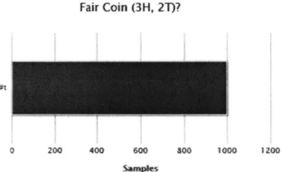
Say you observe five flips of the coin, and note the following outcome: 3 heads and 2 tails. When prompted about the fairness of the coin, since there is really no evidence to support any bias in the coin, most people would respond that the coin is fair. Constructing this model in Church and observing the output backs this fact up, as demonstrated by the histogram in Figure 2-1. The histograms produced by Church in this section will count "#t" and "#f" values, corresponding to "true" (the coin is fair) and "false" (the coin is unfair). As you can see, all 1000 samples from the posterior distribution report that the coin is believed to be fair.

Fair Coin (3H, 2T)?

0 200 400 600 800 1000 1200

Figure 2-1: Results from performing inference on the fairness of a coin. Observed Data = 3H, 2T; Fairness Prior = 0.999

What happens when the outcome changes to 5 consecutive heads? Believe it or not, most people would probably still believe the coin is fair, since they have a strong prior bias towards believing that most coins are fair. Observing five heads in a row is a little weird, but the presented evidence isn't really enough to outweigh the strength of the prior. Histograms for five heads with a strong prior bias towards fairness (Figure 2-2) and with no bias at all (Figure 2-3) are provided below.

Fair Coin (5H, Fairness Prior = 0.5)?

0 200 400 600 800 1000

sames

1200 0 200 400 600 800

sample

Figure 2-2: Results from performing inference on the fairness of a coin. Ob-served Data = 5H; Fairness Prior =

0.999

Figure 2-3: Results from performing inference on the fairness of a coin. Ob-served Data = 5H; Fairness Prior =

0.500

As you can see, both the prior and the evidence are important in determining the posterior distribution over the fairness of the coin. Assuming we keep the expected prior in humans that has a bias towards fair coins, it would take more than five heads in a row to convince someone that the coin is unfair. Figure 2-4 shows that ten heads are almost convincing enough, but not in every case; Figure 2-5 shows that fifteen heads demonstrate enough evidence to outweigh a strong prior bias.

Fair Coin (0OH, Fairness Prior = 0.999)?

0 100 200 300 400 500 600 700

Figure 2-4: Results from performing inference on the fairness of a coin. Ob-served Data = 1OH; Fairness Prior =

0.999

Fair Coin (1 5H, Fairness Prior = 0.999)?

at.

200 400 600 300 1000

Figure 2-5: Results from performing inference on the fairness of a coin. Ob-served Data = 15H; Fairness Prior =

0.999

If someone is generally more skeptical of coins, or if they have some reason to believe the coin flipper is holding a trick coin, their fairness prior would be lower, and the number of consecutive heads to convince them the coin is actually unfair

~1

1000

would be smaller. The essence of Bayesian inference is that both prior beliefs and observed evidence affect the posterior distributions over unknown variables in our models. As the above example should demonstrate, conclusions about the fairness of the coin were strongly dependent on both prior beliefs (notions about fair coins and the existence of a trick coin) and the observed evidence (the sequence of heads and tails observed from flipping the coin).

2.2

Variational Inference

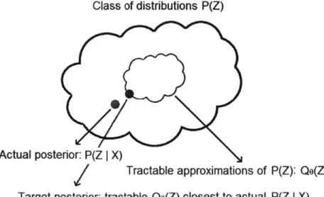
The actual process by which one can infer posterior distributions over variables from prior beliefs and observed data is based on derivations of probability expressions and complicated integrals. One such technique that focuses on approximating those posterior distributions as simpler ones for the purposes of making the computations tractable is called variational inference. Variational inference techniques will result in exact, analytical solutions of approximate posterior distributions. A high-level, intuitive picture of how variational inference works is provided in Figure 2-6:

Class of distributions P(Z)

Actual posterior: P(Z

I

X)

Tractable approximations of P(Z): Qo(Z)

Target posterior: tractable Qe(Z) closest to actual P(Z

I

X)

with

m

( dist ( Qe(Z)

11

P(Z I X)))

The large outer cloud contains all posterior distributions that could explain the unknown variables in a model, but some of these distributions may be intractable. The distributions inside the inner cloud are also part of this family, but the integrals used for calculating them are tractable. The variable 0 parameterizes the family of distributions Q(Z) such that Qo(Z) is tractable.

The best Qo(Z) is determined by solving an optimization problem where we want to minimize some objective function over 0 based on the actual posterior and the family of tractable distributions. The minimum value of the objective function cor-responds to the best possible QO(Z) that approximates the actual posterior P(ZIX).

The best approximate posterior distribution will describe the unknown variable about as well as the actual posterior would have.

The objective function that is generally used in variational inference is known as KL divergence. Other divergence functions can be used, but the KL divergence tends to provide the best metric for determining the best approximation to the actual posterior distribution. The expression for KL divergence is in terms of the target approximate posterior

Q

DKL(QIIP) = Q(Z) log P(X) (2.2)

The optimization problem of minimizing the KL divergence between two probabil-ity distributions is normally intractable because the search space over 6 is non-convex. To make the optimization problem easier, it is useful to assume that Qo will factor-ize into some subset of the unknown variables. This is the equivalent of removing conditional dependencies between those unknown variables and treating the posterior distribution as a product of the posterior distributions. The factorized expression for

Qo

M

Qo(Z) = l q(Zi jX) (2.3)

i=1

'The LaTeX code for the equations in this section come from http://en.wikipedia.org/wiki/ VariationalBayesianmethods

The analytical solution for

Qo(Z)

can show that the approximate factor distributions with minimized KL divergence can be expressed as the following:

eEisa [in p(Z,X)]

q)(Z3 X) =

f

In qj*(Zj

IX)

The intuition behind this expression is that it can usually be expressed in terms of some combination of prior distributions and expectations of other unknown variables in the model. This suggests an iterative coordinate descent algorithm that updates each node in some order, using the updated values of other nodes to refine the value computed at the current node.

This idea essentially describes how variational inference is generally implemented: initialize the expectations of each unknown variable based on their priors, and then iteratively update each unknown variable based on the updated expectations of other variables until the expectations converge. Once the algorithm converges, each un-known variable has an approximate posterior distribution describing it.

2.3

Variational Message Passing

The Variational Message Passing (VMP) algorithm follows the same intuition de-scribed at the end of the previous section: it is an algorithm that iteratively updates the posterior distributions of nodes in a graphical model based on messages received from neighboring nodes at each step.

variational inference surround the use of messages. The nodes in a graphical model interact (send and receive messages) with other nodes in their Markov blankets; that is, their parents, children, and coparents. The messages contain information about the current belief of the posterior distribution describing the current node. As the beliefs change with information received from other nodes, the constructed messages sent out to other nodes will also change. Eventually, the values generated at each node will converge, resulting in consistent posterior distributions over every node in the model.

2.3.1

Message Construction

Constructing the messages sent between a particular pair of nodes is relatively dif-ficult, but by restricting the class of models to "conjugate-exponential" models, the mathematics behind the messages can be worked out. The two requirements for these models are:

1. The nodes in the graphical model must be described by probability

distribu-tions from the exponential family. This has two advantages: the logarithms involved in computation are tractable, and the state of these distributions can be summarized entirely by their natural parameter vector.

2. The nodes are conjugate with respect to their parent nodes; in other words, the posterior distribution P(XIY) needs to be in the same family of distributions as the prior distribution P(Y) (where Y is a parent of X in the graphical model). This has one advantage: iterative updating of the posterior distributions of nodes only changes the values and not the functional form of the distribution.

Once these requirements are enforced, the source of the messages can be directly observed from the exponential family form expression:

In particular, the messages sent from parents to children (Y -+ X) are some function of the natural parameter vector /(Y), and the messages sent from children to parents (X -+ Y) are some function of the natural statistic vector u(X). The other functions in the above expression are for normalization purposes and do not affect the content of the constructed messages.

The natural parameter vector is determined by expressing a distribution in the exponential family form described above, and taking the part of the expression that depends on the parent nodes. The natural statistic vector is determined by taking the expectation of the vector containing the moments of a distribution. The pro-cess for obtaining each vector is different depending on the model in question, but once the vectors are determined, they can be directly inserted into the algorithm implementation for constructing messages.

For derivations of the natural parameter vectors and messages used in the models that the combined VMP/Graphlab implementation can support, see Appendix B for more information.

2.3.2

Operation Details

Determining the content of messages is work that needs to be done before the al-gorithm is actually run on a graphical model. Once the message content is coded into the algorithm, the actual operation of the algorithm follows a specific process that ensures each node in the graphical model ends up with the correct approximate posterior distribution. The steps performed at each node in the VMP algorithm are:

1. Receive messages from all of your parents. These messages will be used in

updating your natural parameter vector during the update step.

2. Instruct your coparents to send messages to their children. This ensures that the children will have the most current information about the posterior distributions of nodes in your Markov blanket when they send you messages in the next step.

3. Receive messages from all of your children. These messages will be summed up

4. Update your natural parameter vector by combining information about your prior with the messages you received from your parents and children. Once the natural parameter vector is current, use it to update your natural statistic vector for future messages you send to any children you have.

The above steps are performed once at each node during a single step of the algorithm. Once all nodes have been updated, the algorithm starts again with the first node. The algorithm terminates either after a set number of steps, or when the natural parameter vector at each node converges to some consistent value.

The update step for a particular node involves updating the natural parameter vector for that distribution. The derivations of natural parameter vectors for specific models supported by the combined VMP/Graphlab code are part of the work detailed in Appendix B. In general, the update step for a given node involves summing all the messages received from your children, and then adding that sum to the initial values of your natural parameter vector.

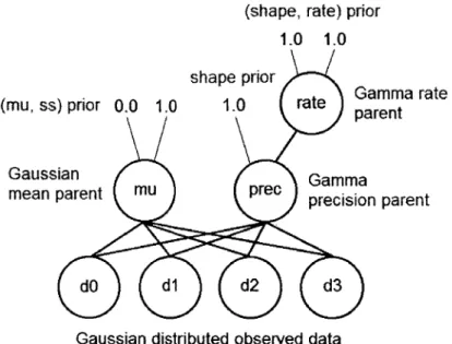
The following example demonstrates how the mu node in a Gaussian-Gamma model is updated during the first step of the VMP algorithm. The graphical model in question is provided in Figure 2-7. The circles with labels are the nodes in the graphical model; the leaf nodes with d, labels are the observed data nodes, and everything else is an unknown variable. The uncircled numbers at the top of the model are the hyperparameters that define the prior distributions over the top-level nodes. The Gaussian and Gamma distributions are part of the exponential family, and the Gaussian-Gamma parent pair for Gaussian-distributed observed data satisfies the conjugacy constraint, so VMP can be performed on this model.

The steps taken for updating the mu node during the first iteration of the VMP algorithm are:

1. The mu node does not have any parents, so do not receive any messages.

2. The children of mu all have prec as a parent, so prec is a coparent of mu and must send messages to the d, child nodes.

(mu, ss

Gauss

mean

(shape, rate) prior

1.0 1.0

shape prior

)

_par

ian _Gamma

parent mu prec precision

dO da d2 d3

Gaussian distributed observed data

mnma rate

ent

parent

Figure 2-7: VMP Example: Gaussian-Gamma Model

3. The d child nodes have been updated, so mu should receive current messages from all of them.

4. The mu node now has all the information about the believed posterior distri-bution of every node in its Markov blanket, so it can combine everything and update its own natural parameter vector and natural statistic vector.

The same steps would apply to prec during the first iteration (with the added note that prec will receive messages from rate in the first step), and the algorithm will keep updating mu and prec during each iteration until the natural parameter vector at both nodes converges to consistent values. The nodes should be visited in topological order during each iteration of the algorithm; in the above example, this means the effective order is {rate, mu, prec}.

As a final note, the observed data nodes already have defined values (we are not determining posterior distributions for observed evidence), so only the unknown variables need to explicitly have an update step. The observed data in the leaf nodes becomes important when the unknown variables directly above them receive messages from the observed nodes; these messages contain the observed data as part

of the message and their upward propagation ensures that the unknown variables in the model take the observed evidence into account.

Chapter 3

Graphlab Distributed Framework

This chapter will describe the Graphlab [33] framework in more detail. The Graphlab framework takes problems represented as factor graphs and executes them on multi-ple cores or machines. The vertices of the factor graph represent individual parts of the problem, and the edges connecting them represent computational dependencies between those parts. The abstraction provided by Graphlab strikes an important bal-ance between flexibility and difficulty in the implementation of parallel/distributed VMP code. This chapter will review some of the basic concepts surrounding paral-lel/distributed computing, and then focus on the design and implementation of the Graphlab framework.

3.1

Parallel/Distributed Computation

The study of parallel/distributed computation involves trying to find ways to leverage multiple processors or multiple machines to solve problems. The "parallel" aspect of computation comes from the processors operating in parallel to solve problems, and the "distributed" aspect of computation comes from multiple computers communi-cating on some kind of network to solve a problem together.

There is usually no straightforward way to convert a parallel program to a dis-tributed one, but as the section on Graphlab will explain later, the Graphlab frame-work abstracts that difference away, allowing programs written with the frameframe-work

to be easily deployed on a cluster of machines. While this makes implementing your program easier, it is still important to have some idea of how each deploy method is different.

3.1.1

Parallel Computing

A typical parallel computing environment will involve multiple processors and some

sort of shared memory that each one will use for reading/writing data. Figure

3-1 demonstrates such a system; the arrows represent the read/write pathways, and

the boxes represent components of the machine (either one of the processors, or the shared memory).

|Processor

Processor

Processor

Memory

j

Figure 3-1: Typical Parallel Computing Environment [28]

The above image doesn't describe some of the concerns that must be addressed when writing parallel programs. For one, correctness is not guaranteed when simply moving a program from a serial environment to a parallel one. When a program is compiled, it becomes a series of instructions designed to run on a particular archi-tecture. When spreading a sequential stream of instructions over multiple streams running at the same time, care must be taken to respect the read/write dependencies between different instructions. Consider the source code example in Listing 3.1:

#include <stdio.h>

void transfer(int *pl, int *p2, int amount)

{

*pl = *pl - amount;

*p2 = *p2 + amount;

}

void main(int argc , char **argv)

{

int *p2 = malloc(sizeof(int)); *pl = 100; *p2 = 100; transfer(pl, p2, 50); transfer(pl, p2, 25); print f(" pl: f/d\n" ,*pl ); print f ("p2: 'od\n" ,*p2 );

}

Listing 3.1: Parallel Dependencies: Transfer Code

When run in a serial environment, the output of the code should be p1 = 25

and p2 = 175. The two pointers have been initialized to hold a total of 200, and that total is preserved when the transfer requests are run in series. If the code above were run in parallel such that each transfer request was executed on a different processor, the results could be different. The lines of code in the transfer function compile down to several assembly instructions each, so there is a high possibility of interleaving instructions. In general, when writing parallel programs, any interleaving of instructions should be assumed possible without locks or other forms of protection. One such interleaving that could cause major problems is when the LD(*pl) in-struction in the second transfer request occurs before the ST(*pl) inin-struction at the end of the first transfer. In other words, the second transfer request may use the old value for *p1 and incorrectly subtract 25 from 100, instead of subtracting 25 from 50. The end result would be p1 = 75 and p2 = 175, which is obviously not what should happen after executing two transfers. There are several other ways to interleave the instructions that could produce incorrect results, so special care must be taken when writing parallel programs.

There are many ways to ensure that shared memory is manipulated in the right order within parallel programs; the most common way involves the use of locks. A lock around some data prevents other processors from reading/writing it until the lock is released. Other examples of concurrency protection will not be discussed here, but can be explored in the references [23, 18, 12].

them, and then release the lock when they are finished. This ensures that the two transfer requests cannot interleave and produce incorrect results. Listing 3.2 shows how locking manifests itself in the above example (of course, the specific implemen-tation depends on the language/framework being used):

#include <stdio .h>

void transfer(int *pl, int *p2, int amount)

{

77

7/

*pl = *pl - amount;

*p2 = *p2 + amount;

/7

7/

}

Listing 3.2: Parallel Dependencies: Transfer Code With Locking

A closer look at what actually happens shows that the program instructions are

actually just run in some serial order. This leads into another concern with parallel programming: efficiency. In the absence of data dependencies, running several parts of a complicated program concurrently should make the program run faster. While parallel programs have some overhead in starting up and combining the results of each processor at the end, that time is easily offset by the amount saved by executing each part of the program at the same time. When dependencies force serialization of the instructions to occur, the overhead becomes an additional cost that might not be worth it.

3.1.2

Distributed Computing

All of the problems described in the parallel computing section are concerns when

writing programs to run on multiple machines. The added level of complexity in writ-ing distributed programs comes from the addition of some communication network

required so that each machine can send messages to each other. Figure 3-2 demon-strates what a typical distributed environment would look like with the same labels for processors and memory used in the parallel computing diagram:

Pmcessor

Memo

~Processo

memory

PProcessor

Memory

Figure 3-2: Typical Distributed Computing Environment [28]

Each of the problems described above (correctness and efficiency) are amplified when working with distributed clusters of machines because the additional require-ment of communication between each machine is difficult to coordinate correctly. Imagine if each of the transfer operations in Listing 3.1 were being run on different machines: there would be significant latency between when one machine updates *p1 and *p2, and when the other machine becomes aware of this update. The lack of actual shared memory between the two machines introduces new problems to the system.

The problem of correctness becomes more difficult to solve because locking mech-anisms will also require communication on the network. A typical solution to dis-tributed locking involves adding another machine to the network whose only purpose is to keep track of which machines hold locks for various data shared over the network. This adds significant complexity to most applications, especially when each machine on the network is performing local operations in parallel with those distributed locks.

The code in Listing 3.2 may still be applicable in a distributed system, but the un-derlying locking mechanism would be significantly more complicated.

The problem of efficiency becomes even more important to consider because the overhead cost now includes a significant amount of time devoted to network trans-mission and message processing. In general, communication networks are assumed to be unreliable, and measures must be taken at each machine in a distributed cluster to ensure every message is received in some enforced order. These measures require extra computation time, and may even delay certain operations from completing. Synchro-nization between multiple machines in a distributed program is another source of computation, and in many cases, this could completely kill any gains realized from an otherwise efficient distributed protocol.

Added to the problems mentioned above is the concern for reliability and fault-tolerance within distributed programs. In a distributed cluster of computers con-nected by a network, both machine and network failures are much more common than individual processor failures in a parallel environment. Accounting for these failures is difficult and requires even more overhead in most systems. While reliabil-ity and fault-tolerance will not be described in any more detail with regards to the VMP/Graphlab system, some useful references can be followed that describe compo-nents of the replicated state machine method for solving this problem [17, 3].

3.2

Parallel/Distributed Frameworks

With all the problems described in the last section, it should come as no surprise that most programs using parallel/distributed environments use pre-existing libraries and frameworks for implementing their code. These libraries and frameworks handle many of the complicated details associated with solving the problems outlined above while providing a high-level abstraction for writing parallel/distributed programs.

In the case of parallel programming, most pre-existing support comes in the form of programming language primitives. In a lower-level language like C, primitive libraries such as pthreads [4] can be used; this library exposes threads and mutexes, but requires

that the programmer explicitly use these constructs to control parallel operation at a fine-grained level. In a higher-level language like Java, the explicit use of locks is not always required, since the language abstracts them away by implementing thread-safe keywords for synchronization [22].

In the case of distributed programming, support within a programming language is not as common, so programs usually incorporate separate systems to handle the details of distributed computing. These systems provide their own abstractions that make the task of dealing with distributed machines way more manageable.

One such example is the Remote Procedure Call (RPC) framework [1], where programs on individual machines make function calls that actually execute on other machines and have the return value sent across the network to the calling machine. Another example is System Ivy [14], where the programs on individual machines access what appears to be shared memory on the distributed network. These ab-stractions require complicated implementations to ensure correct operation, but once completed and tested thoroughly, they can be placed under the hood of other dis-tributed programs and reliably be expected to work.

3.2.1

Distributed VMP Framework

Taking all of the concerns surrounding parallel/distributed computation into account, we needed to find a framework that would seemingly mesh well with the VMP algo-rithm. Three specific frameworks were examined in great detail, with the idea that each one was representative of some class of frameworks:

1. Message Passing Interface (MPI): a low-level framework that provides basic support for sending messages between computers on a network [29]. This frame-work provides no high-level abstraction, but provides a high degree of flexibility since any kind of system can be built around the provided message passing primitives.

2. MapReduce: a high-level framework that reduces the problem of distributed computation to simply providing a map and reduce function to execute in a

specific way on a cluster of machines

[6].

3. Graphlab: a mid-level framework that requires representing a distributed

prob-lem as a factor graph filled with computation nodes and edges describing the data dependencies between those nodes [33]. This framework requires work to represent a problem in the factor graph format, but handles many of the other details of distributed computation once the graph is constructed.

In general, the pattern with most distributed frameworks is that flexibility is usually traded off with complexity. The lower-level frameworks provide simpler prim-itives that can be molded into many different systems, but at the cost of needing to write overly complicated code that needs to deal with many of the gritty details of distributed computation. The higher-level frameworks deal with almost all of those details in their underlying implementations, but at the cost of restricting the kinds of problems they can solve to ones that fit nicely in the provided abstraction.

Using MPI would require that the distributed VMP implementation contain extra infrastructure code for dealing with data dependencies in the variational inference updates. The actual schedule of passing messages would need to be controlled at a relatively low level, so that each node can correctly update itself without using stale data from a previous iteration. This would be difficult, but clearly possible, since nothing restricts the kinds of systems that can be molded around the message passing primitives.

Using MapReduce would probably not be possible because the VMP algorithm has more data dependencies than the underlying structure of MapReduce can support. The MapReduce framework tends to be useful for problems that can be broken down into independently running parts that need to be combined after all processing has occurred. The ease of using MapReduce comes from the restrictive abstraction that only works effectively for certain kinds of problems, so although this framework would remove almost all of the distributed computing concerns, it did not seem useful for

implementing the VMP algorithm.

The Graphlab framework seemed to find a sweet spot between the flexibility pro-vided by MPI and the abstraction propro-vided by MapReduce. The abstraction provides high-level support for distributed computation while actually fitting the problem we need to solve; the factor graph abstraction is restrictive, but seems to mesh well with the emphasis on graphical structure inherent to the VMP algorithm. As men-tioned earlier, the Graphlab framework also provides a way to easily switch between parallel and distributed execution, making it easier to deploy the code in different environments. All in all, the Graphlab framework seemed like the correct choice for implementing a distributed VMP algorithm with the least difficulty.

3.3

Graphlab Distributed Framework

The Graphlab framework, as mentioned earlier, performs distributed computation on problems represented as factor graphs. The underlying implementation of Graphlab handles the concerns described in the parallel/distributed computing section while enforcing an abstraction that "naturally expresses asynchronous, dynamic, and graph-parallel computation" [33]. The majority of the effort in using Graphlab to solve a problem comes from constructing the factor graph to represent a particular problem; an example of an arbitrary factor graph is provided in Figure 3-3.

The numbered circles are the vertices of the factor graph, and the lines connecting them are the edges. Both the vertices and the edges can store user-defined data, which is represented by the gray cylinders in the image (the thin ones with labels Di are vertex data, and the wide ones with labels Die- are edge data). The scope of each vertex refers to the data that can be read and/or modified when a vertex is updating itself during computation. For a given vertex, the scope is defined by the outgoing edges and the vertices connected by those edges. The overall structure of the graph cannot be changed during computation, so the vertices and edges are static.

Once the graph is constructed, the framework performs computation on the struc-ture using a user-defined "vertex program" that uses something called the

Gather-Scope s-

Figure 3-3: Graphlab: Factor Graph Example [33]

Apply-Scatter (GAS) paradigm. The computation model requires that a function be written for each of these three operations. These functions will be called during each iteration of the Graphlab computation on each node in the graph. The purpose of each function is summarized below:

1. Gather: a function that will be called at each vertex once for each of its adjacent edges. Every pair consisting of a node and one of its adjacent edges will call this function before any apply operations are started. This function is typically used to accumulate data from adjacent vertices to be used in an update during the apply step; when the + and + = operations are defined for the declared type stored in each node, accumulation happens automatically and the sum is passed directly to the apply function.

2. Apply: a function that will be called exactly once for each vertex in the graph with the accumulated sum calculated during the gather step as an argument. Every vertex will call this function only after all the gather functions have com-pleted, but before any scatter operations are started. This function is typically used to update the data stored in a vertex. This is the only function whose method signature allows for vertex data to be changed; vertex data structures must be marked as constant in the arguments to gather and scatter.

3. Scatter: a function that will be called at each vertex once for each of its adjacent edges, similar to gather. Every pair consisting of a node and one of its adjacent edges will call this function only after every apply operation has finished. This function is typically used to push new data out to the adjacent edges of a vertex after an update has completed in the apply step. This data will be grabbed by adjacent vertices during the gather step in the next iteration. Similar to the apply step, the edge data structures are not marked as constant in the arguments to this function.

The gather, apply, and scatter functions will execute on each vertex whenever the vertex is signaled. Normally, after constructing a graph, each node will be explicitly signaled once to begin executing some algorithm. The GAS functions will execute one iteration of the algorithm and, unless some convergent value or maximum number of steps has been reached, each vertex will signal itself to run again for another iteration. This signaling mechanism must be explicitly included in the vertex program. When the vertices stop signaling themselves to run, the algorithm ends and the resulting values can be examined in the nodes.

The exposure of the signaling mechanism is an example of how the Graphlab abstraction allows some flexibility to solve different kinds of problems. While there is a standard way for coordinating the signals between nodes so that a typical iterative algorithm can run, an ambitious problem can use fine-grained control of the signals to create interesting update schedules.

Another example of this is evident in the consistency models Graphlab exposes for performing the GAS computations in parallel. While Graphlab handles the compli-cated details of parallel/distributed programming under the hood, the API provides higher-level ways to influence how the computation will actually proceed. This has a direct influence on correctness and efficiency, but it allows the user to find the bal-ance that works best for a particular program. The consistency models provided by Graphlab are outlined in Figure 3-4.

The consistency model chosen by the user directly affects the subset of the scope that a vertex is allowed to read and/or modify during an update step. The

full-Read

Figure 3-4: Graphiab: Consistency Models [33]

consistency model allows complete access to the entire scope of a vertex. This disal-lows the nodes in that scope from executing their own update functions in parallel with the current vertex, providing the highest amount of consistency. This decreases the degree to which parallel computation can occur, so lesser consistency models are provided.

The edge-consistency model is slightly less consistent, only allowing a vertex to modify the data on its adjacent edges, but read all the data in its scope. The edges may still not be involved in parallel computation with this model, however, so a final, lower consistency model is also provided: the vertex-consistency model. The vertex-consistency model only allows reads and writes to occur on the adjacent edges, allowing Graphlab the highest amount of freedom to execute node updates in parallel. In general, consistency and parallelism are traded off differently in each of the consistency models, and the right one to use depends heavily on the constraints of the problem being solved. Figure 3-5 summarizes the trade-off for the three models provided by Graphlab; the highlighted regions represent data that cannot be updated in parallel in the specified consistency model.

The other low-level details of how Graphlab actually constructs the factor graph on a distributed cluster of machines and performs computation with multiple machines

L

Figure 3-5: Graphlab: Relationship Between Consistency and Parallelism [33]

will not be discussed in significant detail, unless it is relevant to some implementation detail of the combined VMP/Graphlab system in Chapter 4.

The next part of this section will outline the PageRank [16] example from the Graphlab tutorial [34] to solidify the intuition behind how the abstraction works and how it should be used to write distributed programs. For more information on the implementation details of the Graphlab framework, follow the reference to the VLDB publication [33].

3.3.1

Graphlab PageRank Example

The PageRank algorithm assigns a numerical weighting to each node in an graph that is based on how "important" the node is relative to the others in the graph. This weighting is determined from some function involving the importance of nodes pointing to the current node and a damping factor included to represent a small ran-dom assignment of importance. For the purposes of this example, the psuedocode provided in the Graphlab tutorial (adapted to look like a standard C program in List-ing 3.3) provides a perfect startList-ing point for implementList-ing this code in the Graphlab framework: