Dynamic loads in layered halfspaces

(1)

DYNAMIC LOADS IN LAYERED

HALFSPACES

by

Sandra Hulleale B.S.E., Princeton University

(1981)

S.M., Massachusetts Institute of Technology (1983)

SUBMITTED TO THE DEPARTMENT OF CIVIL ENGINEERING IN PARTIAL FULFILLMENT OF THE

REQUIREMENTS FOR THE DEGREE OF DOCTOR OF PHILOSOPHY

at the

MASSACHUSETTS INSTITUTE OF TECHNOLOGY September 1985

Copyright @ 1985 M.I.T.

Signature of Author

---

-

I VI

:..- Department of Civil Engineering September 18, 1985 Certified by Accepted by Eduardo A. Kausel Thesis Supervisor MA~$CHUS1'TSiNSTTUT MASSA HUSENS iNSTITUTE

TECHNOLOGY

JAN 0 2 1986

LIBRARIES

Frangois M. M. Morel Chairman, Department Committee on Graduate Students

(2)

Dynamic Loads in Layered Halfspaces by

Sandra Hull Seale

Submitted to the Department of Civil Engineering on September 18, 1985 in partial fulfillment of the requirements for the degree of Doctor of Philosophy.

Abstract

An approximate solution of Lamb's problem of vibrations in an elastic halfspace is presented. The stiffness method of Kausel and Rossset (1981) is used to model a layered soil stratum. The layers are represented by stiffness matrices that are algebraic in the frequency-wavenumber domain. The global stiffness matrix for the soil system is obtained by overlapping the layer matrices at common degrees of freedom. Once the stiffness matrix is inverted with a spectral decomposition, displacements are computed by means of an inverse transform that exists in closed form. The stiffness matrix for an elastic halfspace is derived by taking the Taylor series expansion of the true stiffness about the horizontal wavenumber. The solution for static loads in layered halfspaces is derived by examining the limit of the dynamic case when frequency goes to zero. Modifications of the stiffness matrices for cross-anisotropic materials are presented. Anisotropy is found to cause only changes to the stiffness matrices themselves and not to the underlying mathematics of the displacement calculations.

Examples of displacements for dynamic and static loads are computed and compared to analytic solutions (when they exist). Comparisons show that the discrete stiffness method gives very accurate results with a relatively small ( - 10) number of sublayers in the overlying stratum. A discussion of the limitations of this method and its application to future research topics is presented.

Thesis Supervisor: Title:

Eduardo A. Kausel Associate Professor

(3)

Acknowledgments

I wish to thank Professor Eduardo Kausel, who was superb in his role of advisor. He was generous with his time and inspired in his guidance. I thoroughly enjoyed working and exercising with Professor Kausel.

My financial support for the past three years has been provided by an Exxon Teaching Fellowship.

Mr Clevver he says to Eusa, 'Thats a guvner lot of knowing youre inputting in to that box parbly theres knowing a nuff in there for any kynd of thing.'

Eusa says, 'Thats about it. I dont think theres many things you cudnt do with that knowing. You cud do any thing at all you cud make boats in the air or you cud blow the worl a part.'

Mr Clevver says, 'Scatter my datter that cernly is intersting. Eusa tel me some thing tho. Whyd you input all that knowing out of your head in to that box? Whynt you keap it in your head wunt it be safer there?'

Eusa says, 'Wel you see I cant jus keap this knowing in my head Ive got things to do with it Ive got to work it a roun. Ive got to work the E qwations and the low cations Ive got to comb the nations of it. Which I cant do all that oansome in my head thats why I nead this box its going to do the hevvy head work for my new projeck.'

(4)

List of Figures

Figure 2-1: Geometry of a Layered Halfspace Figure 2-2: Geometry of a Layer

Figure 3-1: Real Part of the True Anti-plane Stiffness

Figure 3-2: Imaginary Parts of the True and the Approximate Anti-plane Stiffness Figure 3-3: Real Part of ki₁

Figure 3-4: Imaginary Part of k,1 Figure 3-5: Real Part of k12 Figure 3-8: Imaginary Part of k₁₂ Figure 3-7: Real Part of k22

Figure 3-8: _{Imaginary Part of k} 22

Figure 3-9: Rayleigh Wave Roots for the True and Approximate Stiffness Figure 3-10: Spurious Root of the Approximation

Figure 3-11: Determinant of the Imaginary Part of the Stiffness for v= 1/4 Figure 3-12: Determinant of the Imaginary Part of the Stiffness for v= 1/3 Figure 3-13: Real Part of the Vertical Displacement at p = 0

Figure 3-14: Imaginary Part of the Vertical Displacement at p = 0 Figure 3-15: Real Part of the Vertical Displacement at p = 1.0 Figure 3-16: Imaginary Part of the Vertical Displacement at p = 1.0 Figure 3-17: Real Part of the Horizontal Displacement at p = 0 Figure 3-18: Imaginary Part of the Horizontal Displacement at p = 0 Figure 3-19: Real Part of the Horizontal Displacement at p = 1.0 Figure 3-20: Imaginary Part of the Horizontal Displacement at p = 1.0

Figure 3-21: True and Approximate Solutions for Vertical Displacements at the Origin Figure 3-22: Displacements Calculated with the Paraxial Approximation for Different

Layer Depths

Figure 3-23: Displacements Calculated with the Paraxial Approximation for Different Poisson Ratios

Figure 4-1: Eigenvalues of Anti-plane Modes for N = 1 to 12 Figure 4-2: Eigenvalues of In-Plane Modes for N = 12

Figure 4-3: Geometry of Homogeneous Halfspace Subjected to Static Point Loads Figure 4-4: Radial Displacements due to Radial Point Load at the Surface Figure 4-5: Tangential Displacements due to Radial Point Load at the Surface Figure 4-0: Vertical Displacements due to Vertical Point Load at the Surface Figure 4-7: Radial Displacements due to Vertical Point Load at the Surface Figure 4-8: Vertical Displacements due to Vertical Buried Point Load Figure 4-9: Radial Displacements due to Radial Buried Point Load

Figure 4-10: Displacements at the Surface due to Vertical Point Load, G. = 2.0 Figure 4-11: Displacements at the Surface due to Radial Point Load, Gr = 2.0 Figure 4-12: Displacements at the Surface due to Vertical Point Load, G1 = 2.0 Figure 4-13: Displacements at the Surface due to Radial Point Load, G1 = 2.0 Figure 4-14: Vertical Displacements versus Depth

Figure 5-1: Real Part of the Vertical Displacement at p = 0, Anisotropic Stratum Figure 5-2: Real Part of the Horizontal Displacement at p = 0, Anisotropic Stratum Figure 5-3: Real Part of the Vertical Displacement at p = 1, Anisotropic Stratum Figure 5-4: Real Part of the Horizontal Displacement at p = 1, Anisotropic Stratum

76 84 92 94 95 96 97 98 99 101 102 103 104 107 125 126 127 128

(8)

-8-Figure 5-5: Real Part of the Vertical Displacement at p = 0, Anisotropic Halfspace 129 Figure 5-6: Real Part of the Horizontal Displacement at p = 0, Anisotropic Halfspace 130 Figure 5-7: Real Part of the Vertical Displacement at p = 1, Anisotropic Halfspace 131 Figure 5-8: Real Part of the Horizontal Displacement at p = 1, Anisotropic Halfspace 132 Figure 5-9: Horizontal Displacement due to Static Horizontal Point Load at the Surface 137 Figure 5-10: Vertical Displacement due to Static Vertical Point Load at the Surface 138 Figure B-1: Homogenous Layer Overlying an Elastic Halfspace 148 Figure B-2: The Root a of Equation B-31 and kh versus a 155

Figure B-3: The Root of Equation B-49 159

Figure B-4: Wavenumber kh 160

Figure B-5: Wavenumber kh versus y 162

Figure E-1: Mapping z from the Right Half Plane to the Left 187 Figure E-2: The Functions Fo(z) and FI(x) for Real Argument 189

Figure E-3: Contours of the Real Part of F0(z) 190

Figure E-4: Contours of the Imaginary Part of F0(z) 191

Figure E-5: Contours of the Real Part of F,(z) 192

(9)

-9-List of Tables

Table 2-I: Table 2-II: Table 2-III: Table 4-I: Table.5-I:

Algebraic Layer Stiffness Matrices A and B Algebraic Layer Stiffness Matrices G and M

Integrals Used to Compute Dynamic Displacements Integrals Used to Compute Static Displacements Algebraic Layer Stiffness Matrices A, B and G

24 25 32 91 121

(10)

-10-Chapter 1

Introduction

The area of geodynamics concerning displacements in an elastic halfspace due to transient loading is known as "Lamb's problem", after the classic work of Lamb (1904). Much work has been done in this field, most of it by seismologists who were interested in describing the propagation of seismic waves in the Earth's crust. These solutions are usually not applicable to engineering problems because of restrictions on the geometry of the soil. The most well known example is the solution of Lamb's problem developed by Cagniard (1962). This method obtains time-dependent displacements due to a transient point source within a solid composed of two semi-infinite homogeneous media in welded contact. When one of these media is assumed to be a vacuum, the solution for a halfspace results.

An examination of the Cagniard method illustrates the features of the transient solution that are important to the study of seismology. The application of this technique starts with the Laplace transforms with respect to time of the wave equation, the boundary conditions and the source. The homogeneous and particular solutions are derived in the transform domain and the boundary conditions are applied. The inverse Laplace transform is not performed, as this would be impossible to do in closed form for most cases. Rather, the variables of the solutions are changed so that the solution takes the form of a Laplace transform, and the inverse transform can be extracted by inspection. This change of variables usually requires several applications of conformal mapping and contour integration, which render the mathematics of Cagniard's method formidable. Dix (1954) presented a simple application of Cagniard's technique to the solution of the scalar wave generated by a point source in an infinite medium. Dix also explained how the solution for a general transient load can be obtained by applying the Duhamel integral to the solution for a step load. deHoop (1962) modified the method of Cagniard by applying Fourier transforms to the

(11)

-11-spatial variables as well as a Laplace transform with respect to time. The inverse Fourier transforms are then manipulated with changes of variables into a Laplace transform and the solution is extracted by inspection. deHoop also applied his method to the solution of a scalar wave in an infinite medium.

Johnson (1974) presented the full three-dimensional solution, derived with the Cagniard-deHoop method, for displacements in a halfspace due to a unit pulse. In this work, the advantages of this technique to the study of seismology become clear. The solution for displacements is given as the sum of six wave forms: incident P and S waves and reflected PP, SS, PS, and SP waves. Thus the progress of a particular wave can easily be examined by separating this wave from the displacement solutions. Although the solution method tends to lose physical meaning during the multiple integrals performed in the complex plane, the final result for displacements is expressed in terms of normal modes of wave propagation that are easily understood. The references cited above give examaples of displacement solutions that exist in closed form for special cases (e.g. at the surface). The general solution given by Johnson contains an integral which must be evaluated numerically. The fact that the Cagniard-deHoop method is restricted to a homogeneous halfspace and requires numerical integration makes it less practical for engineering applications where displacements in layered soils are desired.

Another solution for dynamic loads in a homogeneous halfspace was developed by Pinney (1954). Integral solutions for layered halfspaces have been given by Bouchon (1981), Luco and Apsel (1983) and Apsel and Luco (1983). Alekseyev and Mikhaylenko (1976/1977) developed a procedure that can be used in a finite difference formulation and Whittaker and Christiano (1979) employ the integral Green's function of the halfspace in a finite element method for flexible plates. All of the above methods require numerical integrations of improper integrals. This is a difficult problem, since the integrands involve transcendental functions which themselves must be evaluated numerically and the kernels may be "wavy", leading to high computational effort for proper resolution of the integrals.

(12)

-12-Transfer matrix techniques are another approach to the problem of displacements in layered halfspaces subjected to dynamic loads. Thomson (1950) and Haskell (1953) developed a transfer matrix that relates the state vector (the stresses and displacements on an interface) of a layer to the state of the layer above it. The elements of the matrix are transcendental functions of the frequency w, wavenumber k and layer properties. Since the matrix is written in the frequency-wavenumber domain, integral transforms are required to obtain displacements in the space-time domain. _{Applications of the transfer matrix method have been presented by Harkrider (1964),} Haskell (1964), Knopoff (1964) and Dunkin (1965). Although the matrix method simplifies the problem of layering, numerical integration is still required to obtain displacements.

The starting point for the solution method described in this paper is a stiffness matrix derived from the Haskell-Thomson transfer matrix by Kausel and Roisset (1981). Elements of the transfer matrix are rearranged so that stresses on two adjacent interfaces are related to displacements on the interfaces via the stiffness matrix. Then stiffness matrices of the individual layers are overlapped to form a global stiffness matrix for the soil system. The stiffness method is analagous to the matrix techniques applied to problems in structural dynamics. Displacements are computed with numerical integration. Details of the method are presented in Chapter 2.

When the thicknesses of the layers in the soil are small compared to the wavelengths of interest, the transcendental functions in the stiffness matrix can be simplified to algebraic functons of the wavenumber k. This is accomplished by making the assumption that the displacements are piecewise linear in the vertical direction. The algebraic stiffness matrices which result were first presented by Lysmer and Waas (1972). Waas (1972) and Kausel (1974) also derived these matrices. The matrices have been used to represent the behavior of semi-infinite boundaries in finite element analyses by Drake (1972), Schlue (1979), and Tassoulas (1981).

The algebraic stiffness matrices have also been applied by Kausel and Peek (1982b) to obtain Green's function solutions of layered soils resting on a rigid base and subjected to dynamic loads. The method described here and in the above reference is a specialization of the one presented by

(13)

-13-Kausel (1981). The global stiffness matrix of the stratum is assembled and the harmonic applied load is transformed into the wavenumber domain. The stiffness matrix is inverted with a spectral decomposition in terms of the natural wavenumbers and propagation modes (the eigenvalues and eigenvectors of the stiffness matrix). The inverse integral transform is then performed to yield displacements. The principal advantage of this method is that the inverse transforms exist in

closed form, thus increasing the speed and accuracy of the procedure. This method was applied by

Kausel and Peek (1982a) to obtain Green's functions for use in a boundary integral method for layered soils.

The technique described above has been limited to cases of a soil stratum resting on a rigid base, since no thin layer approximation can be made to a halfspace. This paper describes an extension of the method to dynamic problems of layered soils resting on a viscoelastic halfspace. The algebraic expression of the halfspace stiffness is obtained by taking a Taylor series expansion of the true transcendental stiffness. Then a solution for static loads in layered halfspaces is obtained by evaluating the dynamic case in the limit when the frequency w goes to zero. Finally, an extension of the method for anisotropic media with as many as five elastic constants is presented.

This method for computing displacements due to dynamic loads in layered halfspaces is an engineering solution to a well known problem. The accuracy and speed of the solution method make it useful for a variety of engineering problems which are described in this paper.

(14)

-14-Chapter 2

Review of Previous Work

In this chapter the assumptions and the mathematics leading to the Green's function solution of the stratum are presented. For more detailed theory on the propagation of waves in elastic media, the reader is referred to Aki (1980), Bith (1979), Graff (1975), Love (1944), Love (1967), Bullen (1963) and Pao (1983). Studies of the propagation of waves in layered media can be found in Brekhovskih (1980), Ewing et. al. (1952) and Ro~sset and Kausel (1980). The essential mathematics, distilled from the above references, are given below.

2.1 Geometry and Material Properties

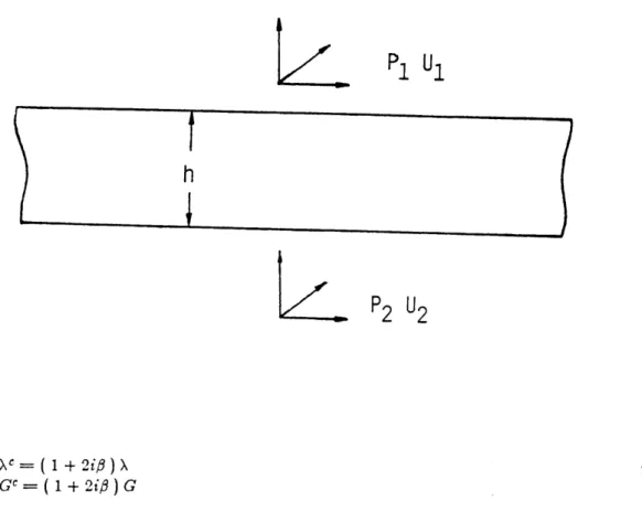
The geometry of the halfspace is shown in Figure 2-1. The surface of the halfspace, where z = 0, is the xy plane in Cartesian coordinates, or the p-6 plane in cylindrical coordinates. The cross-section of the halfspace, in Figure 2-1 is the z-x or z-p plane. The stratum resting on the halfspace has total depth H and is subdivided into N parallel layers. The layers are numbered sequentially with layer 1 being at the surface and layer N being above the halfspace. The layers are in "welded" contact such that displacements and stresses are continuous across the layer interfaces. Figure 2-2 shows the geometry of an individual layer with loads and displacements at the interfaces. Each layer i has depth hi and the interface elevations are z; and

zi+1-The individual layers are homogeneous. Each layer i has mass density denoted by pg. For isotropic layers (see Chapter 5 for a discussion of anisotropic materials), each layer has Lam6 constants X; and G,, with the corresponding Poisson ratio v; and elastic modulus Eg. To model the dissipative behavior of soils, we use the complex Lam4 moduli

(15)

(16)

-16-Figure 2-2: Geometry of a Layer

P

₁

_U

₁

P2

U

2

X= (1 + 2ip) X

Gc=

(

1 + 20) G

where # is the fraction of critical damping. For w > 0,

#

is also positive. Since the damping coefficient is independent of frequency, damping is hysteretic in nature. For more details on hysteretic damping, see Kausel (1974). Using complex moduli to represent a linearly viscoelastic material does not alter the derivations presented for a linearly elastic material. Thus the complex moduli can be substituted for X and G when dissipative behavior is required. The use of complex moduli in cases of dynamic loading insures that no singular displacements (at resonance) are obtained.

2-1 I

(17)

-17-2.2 The Stiffness Method

2.2.1 In-plane Motion

Consider a stratum in plane strain subjected to a harmonic load. The displacement vector in Cartesian coordinates is

u(X,z) 0 w(x,z)

2-2

where w is the frequency of the forcing function. Motion is restricted to the x-z plane and is independent of the y coordinate. In layer i, the wave equations are

(Xi + 2G;) T + Xi

azaz

+ _8x(9zg92 _I++ pp2U = 0

(Xi + 2G;) Z2 + Ai X89z + Gi 8 2

W 82U

iX

2 ₊_azaz + PW2w = 0 The stresses are given by

eou e8w ex= (Xi + 2G;) a + XA ;~ i (9w +ou T.z = G(9z 9 & aw

ou

or, (Xi + 2G;) 9 + XA

We look for solutions by separating the x and z dependence of the displacements

u(x, z) = U(z) f(x)

w(x,z) = W(z) f(x)

Substituting 2-5 into the differential equations 2-3 gives

dx2 + k2f = 0

where k is a constant (the wavenumber). Thus the displacements are given by

2-3 2-4 2-5 2-6 (g2U G; gI Z +

(18)

-18-u(x,z) = U(z) e-ikx

w(x,z) = W1z) e-ik.

Now write u and w as

U=

az

- 8z

a

= z+

ax

where # and ?P are potential functions. obtain

ax

2

+ 892 = -C #P

When 2-8 are substituted into the wave equation 2-3, we

2-9

ax

2

+ z2 = -C2 V 81

where C,; and C are the shear and pressure wave velocities, given by

G.

X.+ 2G.

We want to find solutions to 2-9 of the form

#(X,z) = O(z) e-ik 7P(X,z) = tp(z) e-ikz

Substituting 2-11 into 2-9 gives

dz2 dz2 + r 2= 0 + S 2 = 0 where 2-7 2-8 2-10 2-11 2-12

(19)

-19-W2 r = -~~ - k2 2-13 PS W2 Ce2= - k2 8z

Then the solution for the potential functions is

4P(z) = Ali cos (rgz) + A2 sin (riz) 2-14

I(z)= A3; cos (siz) + A4; sin (Ygz)

Substituting 2-14 into 2-11 and then applying 2-8, we obtain

d V

U = -ik - dz 2-15

dP

W = d - ikt

The amplitudes Alg, A2 , A3g, A4; for each layer i can be expressed as functions of U(z.), WV'z;), U(zi+1), WVzi+1 ) and also as functions of uz(z;), rz(z;),

az(zi+1),

Tzz(zi+1). This is the basis of the transfer matrix. The state vector, Zi+1 = { is obtained in terms of the amplitudes A. Then the amplitudes are obtained in terms of the state vector Z;. This amplitude vector is then substituted into the expression for Zi+1 to yield

Zi+1 = H; Z; 2-16

where Hi is the local transfer matrix. The elements of the transfer matrix can be found in Haskell (1953).

2.2.2 Anti-plane Motion

Consider a stratum in anti-plane shear subjected to a harmonic load. The displacement vector is

V(X'Z)

eZ-''

2-17

(20)

-20-Motion is in the y direction and planar (independent of the y coordinate). The equation of motion in layer i is

G; 5 + a] - p1{w

2

V =0 2-18

The shear stresses are given by

av

T = G;&2-19

Separation of variables gives a solution of the form

v(x,z) = 1(z) e-ikz 2-20

From the differential equation 2-18, we obtain the function

1(z) = Ali cos (siz) + A2 sin (sgz) 2-21 where

2 2

8. 2 - k

at

Again, Ali and A2i can be removed from the expressions for v(zi), v(zi+i), Ty'(zi), ry,(zi+1) so that v and rzat zjlare linear functions of v and yat zi.

2.2.3 Development of the Stiffness Method

In this section, a summary of the technique developed by 1'ausel and Roi~sset (1981) is presented. The reader is referred to that reference for more details. Adopting the notation of Kausel and Roesset, we write the state vector as

2yz

T

-

2-22

(21)

-21-in Cartesian coord-21-inates and

Z =

{

LUg 8, , z -=pz

[zv

_2-23

[U

in cylindrical coordinates. The superscript bar indicates that these quantities are functions of z only. In Cartesian coordinates, for a stratum in plane strain, the true state vector is

S e i(wt - kz) 2-24

where w is the harmonic frequency of the forcing function and k is the horizontal wavenumber.

In cylindrical coordinates, the dependence of the displacements and stresses on the azimuthal direction is given by multiplying , iz> Tpz, a2 by cos p6 and up, 7# by -sin p9 if the displacements and stresses are symmetric with respect to the z axis, or by sin PO and cos p9 if they are antisymmetric. The integer p is a Fourier index which is described below. The variation in the radial direction is given by multiplying V and S by the matrix C,, which is the same for all layers

[u]_ [22w

[-

2-5

2J

U CpU C, SI C~ C, ~~ C, [-25S where [~)i j~ 0

]2-26

d1 d CP |kp Ip d(kp) Jp 0 0 ₀ _-J,

j

and J, are Bessel functions. Thus the displacements and stresses are decomposed into a Fourier series in the 0 direction and into cylindrical functions in the p direction.

(22)

-22-Zj+1 = H Z 2-27

where now the vectors contain all three displacements and continuous stresses. In plane strain, the in-plane motions are uncoupled from the anti-plane motions, as described in the section above. The transfer matrix for cylindrical symmetry is the same as that for plane strain. The transfer matrix is not a function of the Fourier index yi.

Now we consider equilibrium of a single layer. The layer has load P = S I on the upper interface and P 2 ~ 2 on the lower interface. Then, substituting in 2-27, we obtain

[1H][

H12

U-1

_2-28

-P 2 ~ H21 H22 P-1

where Hg are submatrices of H, obtained by partitioning. Rearranging terms so that loads are on the left hand side of the equation gives

-1-H

H

1 [

I

1 S1

₁₂ U 2 2-29

2H22H12H11-H21 -H22H

-or

P =KU

where K is the symmetric layer stiffness matrix, P is the load vector and U is the displacement vector. The global stiffness matrix for a layered soil system is formed by overlapping the layer

matrices at common degrees of freedom. The global load vector consists of tractions applied at the layer interfaces. The techniques applied to solve for displacements are analagous to those of structural dynamics. The elements of the K matrix are complicated transcendental functions. The

(23)

-23-2.3 Green's Functions for a Layered Stratum

In this section, the algebraic stiffness matrix is presented and it is applied to the solutions of displacements in layered stratum subjected to dynamic loads. The material in this section is taken from Kausel and Peek (1982b).

2.3.1 Algebraic Stiffness Matrix

When the soil layers are thin compared to the significant wavelengths, the layer stiffness matrix can be approximated as

K- = A-k2 + B k + G -- w2 M. 2-30

These layer matrices are computed by assuming that displacements are piecewise linear in the z direction and then applying finite element energy balance techniques. The displacements in layer

j

are

__ zi+1 ~ z __ z - zg _

U = h U j+ h U j+1 2-31

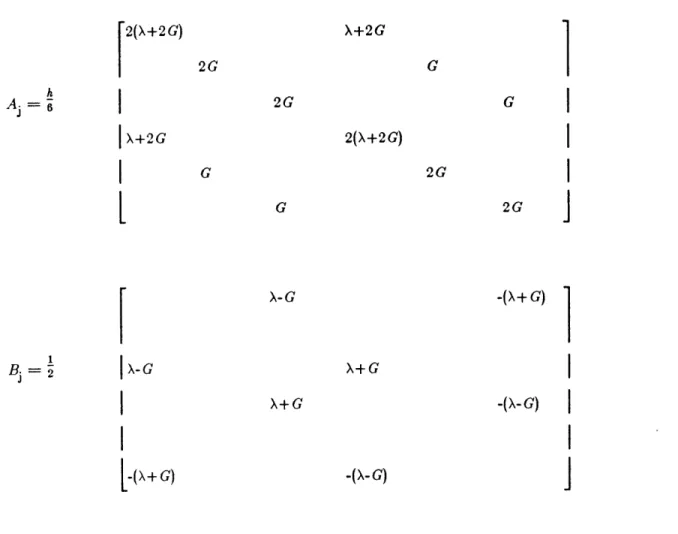
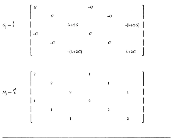
Each layer is a one-dimensional finite element in the z direction. The layer stiffness matrices A; and B1 are presented in Table 2-I, G. and M. are presented in Table 2-I. Note that the 2nd and

5th rows and columns of these matrices, corresponding to the anti-plane degrees of freedom, are uncoupled from the in-plane degrees of freedom.

The global stiffness matrix is assembled by overlapping the layer stiffness matrices at common degrees of freedom. For the stratum resting on a rigid base, the three degrees of freedom at the interface of the rigid rock are set to zero and removed from the eigenproblem. Note that when the wavenumber k is zero (no propagation in the x direction), the stiffness matrix G - w2A is that of a vibrating shear beam modeled with finite elements and a consistent mass matrix. Thus the layered stratum has the same resonant frequencies as a shear beam with a fixed base.

(24)

-24-Table 2-I: Algebraic Layer Stiffness Matrices A and B

2(X+2G)

X+2G X+2G 2G 2G 2(X+2G) 2G X-G X+G

[-(X+G)

G

2G

-(X+G)

-(X-G)

-(X-G)

In principle, for a vector of prescribed extermal loadings P , we wish to obtain the displacements U by inverting the stiffness matrix

U = K-1 P 2-32

This inversion is performed with a spectral decomposition of the stiffness matrix. In order to obtain the wavenumbers and modes of propagation, we must solve the quadratic eigenvalue problem

h

A.= ₈

1

(25)

-25-Table 2-II: Algebraic Layer Stiffness Matrices G and M

G

-G X+2G -(X+2G)

2 -(X+2G)

X+2G

1

2 J

K g = 0 2-33

For a stratum of N layers, the solution of this problem yields 2N eigenvalues for the anti-plane case and 4N eigenvalues for the in-plane case. The wavenumbers ki occur in pairs of *kg, which correspond to waves that travel from the origin and decay towards infinity and waves that travel from infinity and decay towards the origin. The details of the eigenvalue problem and physical siginificance of the wavenumbers are explained in detail by Waas (1972). We select the 3N eigenvalues kg with negative imaginary part for complex kg and positive real part for real ki. These

1 Gj= h

(26)

-26-correspond to waves that propagate away from the origin or decay towards the origin.

The quadratic eigenvalue problem can be expressed as a linear eigenvalue problem of double dimension, which requires all 6N eigenmodes for decomposition. The special structure of the matrices in this case allows the quadratic eigenvalue problem to be expressed as a linear problem of the same dimension. Rearranging the rows and columns of the stiffness matrix by degree of freedom, we obtain the eigenproblem with right and left vectors

K Z,=(A k2 +C ) Z =0 2-34 .K=Y

(

A k + C

)=0

where AX

A= B

X

Az

_2-35

C, Bzz CZ

and the submatrices are all tridiagonal. For a given frequency w, C= G - w2M. The left and

right eigenvectors are

r

_rjxj

_1~

Y. [

$j

Z

=

k;4zij

2-36

Oyj Oyj

In matrix form, the eigenvalue problem is

A~ Z K2+ C Z=0 2-37 A T y K2 + i-TY= 0 where [.KR] Y Oz

(27)

-27-Z

=[P:KR

_2-38

K

[KR

"Rayleigh" modes

K] = "Love" modes

Kausel and Roosset (1981) derived the group velocities (velocities at which energy is transferred into the medium) of the natural modes of propagation from the eigenvalue problem. The left and right eigenvectors satisfy orthogonality with respect to A and C . The normalization is

yTIA Z= IKR] = J _2-39

YTC~Z=- KR 2 = JK2

From 2-39, we know that A and C can be inverted when no eigenvalues are zero. The results of inverting A and C are given by Kausel and Peek (1982b). The equilibrium equation 2-29 in the wavenumber domain is ={~k 2 + )U~= p 2-40 where U ,P, [ = /kU z P kPz 2-41 U Y P Y

We premultiply 2-4 by YT and postmultiply by Z Z-1 = I to obtain

yT( X k2+ 4

-)

Z Z-1 _~_=YT

2-42

Applying the orthogonality relations 2-39 to 2-42 yields

(28)

-28-Solving for displacements U in the wavenumber domain gives

U = Z J- 1 ( k2 I - K2 )-1 yT7

Expanding 2-44 yields the flexibility (the inverse of the stiffness) matrix

T IJ z k4izKRDR

iD~

=~ T#~~g y ' kO K--lD 0 T ,,ZDR z 2-45 TyDL I PI D =(k2I-K2 1-j DR = (k2I-K2 )-1

It can be proven that this flexibility matrix is symmetric. We define the N X N submatrices

F,= {f ""}=D T m,n =1,..., N F=

{

=

{

1i 1_Di z kLxK RIDRO mnz =z X{ 1-DRf= m

}

zz Fzz = {f z} FYY = {f 4n } = OyD Te 2-46 2-47

The elements of the flexibility matrix for displacements at the mth elevation due to loads at the n t elevation are

[f

mn

;cni

F""= 0 m" 0 2-48

mny mn.

fz 0 fz

The matrices of eigenvectors are

1= 1, . . . ,2N

2-44

where

(29)

2-50

-29-2-49 #2 = { #"" m = , .. . ,N 1= 1,.. .',2N

Su={i#t} m2=-,9. .d. ,2N l 1 .. . fN

Substituting 2-49 and 2-46 into 2-47 yields the individual elements of the flexibility matrix

2N mn _ Onl Oni aR 1=1 2N 2N

f

m =

(

4 n4

b

= " $I cRR-1=1 1=1 mn m Oni aR z'z z z 1=1 N = m 76n1 qMfll aL 1=1 where 1 1 k, a, = k2 - k2 k, k2 - k 2) k ( k2 - k 2 ) 2-51 Now that we have obtained the inverse of the stiffness matrix, we can proceed to solve for displacements.

2.3.2 Solution for Displacements

At this point, we matrix, and therefore cylindrical coordinates.

make a switch to cylindrical coordinates. As stated previously, the transfer the stiffness and flexibility matrices, is the same for plane strain and

The stress and displacement vectors are

S =T ez U = Up

The Hankel transforms between the wavenumber and the spatial domains are

U= T k CIO U dk

p=o

2-52

(30)

-30-U = a, p C, f TP U dO dp 2-54 where p is the Fourier index, C. is the matrix of Equation 2-26 and T, is a diagonal matrix containing the terms cos p and sin p0 according to the symmetry of the loading, as described in

Section 2.2.3. The orthogonalization factor a. is

1

(2i

for p=0

ap= 2-55

for yy 0

The time dependence of the loads is the constant factor eiwt.

By applying the results of the previous section, we obtain the displacements at elevation m due to a load applied at elevation n

U"

=

T

k C, "n p dk

2-56

y=0

where P . is the load vector in the wavenumber domain,

oo ₂

P P= a j p CP T, P d dp 2-57

The advantage that the method presented above has over the ones cited in Chapter 1 is that the transforms of Equation 2-56 are computed in closed form.

Consider a horizontal and a vertical disk load. The components in cylindrical coordinates of uniform loads q over a disk of radius R are

r

cos

0 r

0

i

PH q -sin

J0

PV=q 0 0

<

p R 2-58

10 1

The transform of the horizontal load, from 2-57, is

P~= q 1 k J(R) 2-59

(31)

-31-P

,=

0

i =4

1

The transform of the vertical load is

~P = -q 0 k J,( kR) 2-60

0 RLL

1

P, 0 y -74 0

Substituting 2-59 into 2-56, we obtain the displacements due to a horizontal disk load

u"= qRd$"$ N (cos 0) 1=1 1=1 r 4 2N ,i Omo .1 N l 1

~

-i )26 1=1 1=1 u = -qR y $"s$ (c + OR 0) 1=1

Likewise, substituting 2-60 into 2-56, we obtain the displacements due to a vertical disk load up qR O( O $" kg ,1$ d p Y 3

1=1

un "=0 2-62

u qR 0,$"n I k (Co

Kausel and Peek (1982b)). Note that stresses can be obtained from this solution for displacements. Derivatives can be taken in the 2 direction once, and the solution is continuous in the p direction. Thus stresses can be obtained at the center of each layer.

The computation of these Green's functions is a simple procedure: 1. Assemble the global stiffness matrix. 2. Extract eigenvalues and eigenvectors. 3. Evaluate the formulas in 2-61 and

(32)

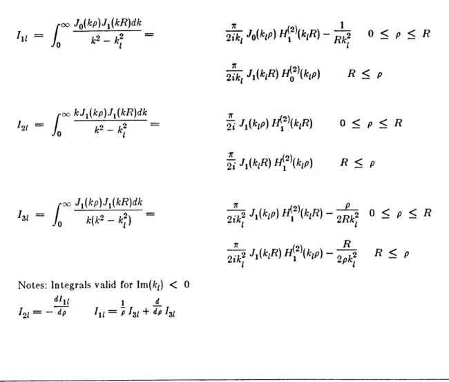
-32-Table 2-III: Integrals Used to Compute Dynamic Displacements

oo Jo(kp)J(kR)dk Igg = k2 - k2 fo I - J(kp) Hd2)(kR) -2ik (k ₁ _RkI oo kJ1(kp)J1(kR)dk 1st=1 _k2_{- k}₂ oo J1(kp)J1(kR)dk I31 = k(k2 - k = J1(R _{_(2)}_{(ki p)} -ik J( I ) H 2{i ) J7(r R H2)(kip) 2ik J(kg ) H2)(k) V 1 2ik _7rI 2 J, (k ₎ _(ip_tL. R < p 0 < p

<

R R < p 2 2Rk 2 R - 2p₁2

Notes: Integrals valid for Im(kj) < 0

12 1 d p I =I 1I3 + d p 13j

Displacements computed with this procedure are compared to those computed with numerical integration of the transcendental stiffness in Kausel and Peek (1982b). Plots of displacement versus frequency at different radii are presented. For the stratum, very accurate results are obtained with a relatively small number of layers ( - 12). The resonant properties of the stratum at its shear beam frequencies are well reproduced. It is also shown that the discrete solution diverges when waves with wavelength X less than 4h dominate the motion. The discrete solution is shown to save great computational effort over the continuum solution for situations where the

0 < p < R

0 < p

<

R R < p

(33)

(34)

-34-Chapter 3

Dynamic Loads in Layered Halfspaces

Two approaches to the solution for dynamic displacements in layered media have been discussed in this paper. The most widely employed techniques involve integral transforms which must be evaluated numerically. In Chapter 2, a method developed by Kausel was described where the transforms exist in closed form. However, this method is restricted to situations where the soil layers rest on a rigid base. Davies and Banerjee (1983) presented a review of several of these techniques applied to the solution of dynamic displacements in a halfspace. They used Kausel's method to study a halfspace by modeling the soil deposit with a very large depth so that the rigid base had little influence on the displacements near the surface. The relatively large depths of the bottom layers introduced numerical inaccuracies in the solution. The accuracy of the solution improved as the number of layers was increased.

An alternate approach is to derive algebraic approximations for the impedance of the halfspace itself. The contribution of the halfspace stiffness to the bottom interface can then be added directly to the global stiffness matrix of the layered soil system. Thereafter, the procedure for calculating the Green's functions is exactly the same as for the rigid base case described in Chapter 2. The procedure given below has been presented by Hull and Kausel (1984) in an abbreviated form.

The approximation to the halfspace stiffness is called a "paraxial" approximation because it is valid for paraxial waves, or waves that propagate within a cone of the z axis. A paraxial approximation of the wave equation that is used as an absorbing boundary in a finite difference scheme was presented by Clayton and Engquist (1977). They employed the approximation to absorb the energy of incident waves on the boundary of the finite difference grid.

(35)

-35-3.1 Derivation of the Paraxial Approximation

A second-order paraxial approximation to the halfspace stiffness is obtained by calculating the first three terms in the Taylor series expansion of the exact impedances:

1

K(k) ~ K(O) + k K'(O) + i k2 K"(O) 3-1

where the primes indicate derivatives with respect to the wavenumber k. The exact impedances are given by Kausel and Ro~sset (1981). For the anti-plane case,

K = k s G 3-2

And for the in-plane case,

[K

- 2(G 1 - s) [ r s2 1 01 3-3

where G is the shear modulus of the halfspace. The parameters r and s are defined as

r = '1 - (w/k C,)2 3-4

8= 1-(w/k C)2

where w is the frequency of excitation. The mathematical details of obtaining derivatives and evaluating them at k = 0 are presented in Appendix F. For the anti-plane case, the paraxial approximation is

G w G C,

G8

K (k)~.-i~ - i 2 k2 3-5

For the in-plane case, the paraxial approximation is

[1

+ ( - 2a)

1

_G

_C

_[-(2

_-

_a)

1

K(k) pC 1

I/ai

1/a]+G

a

]+i2ak

a

2

[

(1 - 2a)/a2

3-6

CO

where a = ~c is the ratio of the s-wave speed to the p-wave speed. p

(36)

-36-be equivalent to the paraxial approximations to the wave equation developed by Clayton and Engquist (1977) (actually, there is a sign error in the Clayton-Engquist approximation which is discussed in Appendix G). In the approximation 3-6, the terms in k and k2 fall on the diagonal and the terms in k1 fall on the off-diagonal. Thus, when these matrices are added to the global stiffness, the structures of A, B and C remain the same as in the stratum case. All of the techniques described by Waas (1972) can still be applied to solve the eigenvalue problem.

The stiffness matrix as a function of k = 0 represents the behavior of the halfspace when displacements are functions of frequency only, i.e. during standing waves. The iw term indicates that the halfspace acts as a dashpot, absorbing energy in the form of radiation damping. The other terms in the paraxial approximation do not have straightforward physical interpretations. The behavior of the approximation as a whole is investigated below.

3.2 Characteristics of the Paraxial Approximation

3.2.1 Anti-plane Case

Clayton and Engquist (1977) show that the range of acceptable wave velocities for the scalar wave equation is C < C,. For wave velocities greater than the shear wave speed of the material, evanescent waves are obtained. This dissipative property is not physically possible in the undamped halfspace. We define the dimensionless parameter X

C, k C8

X = W = C 3-7

In terms of X, the exact halfspace stiffness is

K(X) = wpC, VX2 - 1 3-8

The paraxial approximation is

K(,\) c_- iopC, 1 - i

X23-[

(37)

123-

-37-Expanding in Taylor series about small k has the same effect as expanding about small X, so we expect the paraxial approximation to best represent the true stiffness when X is small. Figures 3-1 and 3-2 show the real and imaginary parts of the anti-plane stiffness. It is clear from 3-8 that the true stiffness is real when X > 1, which is outside of the range of interest. The real componenet for X > 1 is shown in Figure 3-1. From 3-9, we can see that the approximation of the stiffness is always imaginary. The plot of the approximation and the imaginary part of 3-8 is shown in Figure 3-2. For values of X less than 1, the agreement with the true stiffness is excellent.

Another test of the quality of the approximation is an investigation of the roots of the stiffness matrix. By setting the determinant of the stiffness matrix to zero, we obtain the velocities at which waves will propagate parallel to the traction-free surface of the medium. For the anti-plane case, this reduces to setting K(X) to zero. From 3-8, we see that K(X) is zero when X = 1. In other words, anti-plane shear waves propagate parallel to the surface of a halfspace at the shear speed of the soil. The approximation 3-9, on the other hand, has one root at X = V2-. Thus, in the

algebraic model, shear waves propagate at approximately 1.41 times the material shear speed.

The energy absorbing characteristics of the approximation are important for deciding how well it models a halfspace. Waas (1972) showed that the energy transmitted by propagating waves

in a layered soil is (in the most general case)

E = Im { u* K T

}

3-10

where the * indicates the complex conjugate transpose of the displacement vector. This is a quadratic Hermitic form involving a complex, symmetric matrix. Hence, its imaginary part, for arbitrary complex u, is only a function of the imaginary part of K. In particular, the determinant of the imaginary part of K should be greater than zero in order to insure positive definiteness of the quadratic form, i.e., to guarantee a positive energy transmission for arbitrary displacements u. In matrix form, this is

(38)

REAL PART OF ANTI-PLANE STIFFNESS R(K)

I

.5 -0.5. -I .0. -1.51 0.2 POISSON MOD EQUALS 0.25 0.4 0.6 0.8 1.0 1.2 EXACT -APPROXiM .4 1.6 LAMBDA

I

, I

(39)

IMAG PART OF ANTI-PLANE STIFFNESS EXACT

I

(K) APPROXIM 1.0. og 00 . . 0.0 -0.5 -0.8. -1.0 0.2 0.4 0.6 0.9 1.0 1.2 1.4- 1.6

PMISSON MOD LAMBDA

(40)

-40-For X < 1, the imaginary part of K(X) is

WpC, V1 -

X2

3-12

which is always positive (frequencies are understood to be positive). The imaginary part of the approximation is

wpC, 1[ X2 3-13

which is positive for X2 <

V2.

In the range of interest, X < 1, the imaginary part of the paraxial approximation is indeed positive. Thus the paraxial approximation absorbs energy from the waves as does the elastic halfspace.

The dispersion relation, obtained from the wave equation, for the anti-plane case is

2 W2

k2X + k = 2 3-14

Clayton and Engquist (1977) show that the paraxial approximation best matches Equation 3-14 for small values of k.. This means that for small values of k., the paraxial approximation behaves most like the wave equation. The advantages of this attribute are not evident for the present application.

3.2.2 In-plane Case

In terms of X, the exact stiffness matrix for the in-plane case is

K(X)= wpC,

X

1 -

r

1 ~

2 ]

3-15

where

e X2 3-16

a2 Cak C,

(41)

-41-The paraxial approximation is

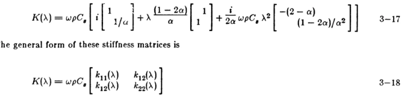
K(X) wpC441 ]+X (1 - 2a) [12 [ -(2 - a)

a-K(X =wp, ie X a i + 2a WpC, (1-2 2 a/2 3-17

The general form of these stiffness matrices is

[

k

11

(X) kis(X)1

K(X) = wpC' k12(X) k22()

J

3-18

Figures 3-3 through 3-8 show the elements of the stiffness matrix as a function of X for the exact and the approximate cases. The elements are computed for a Poisson's modulus v equal to 0.25 (a - 0.57735). Figure 3-3 shows the real part of ki and Figure 3-7 shows the real part of k22. Figure 3-4 shows the imaginary part of k₁_{l and Figure 3-8 shows the imaginary part of k}

22. From Equation 3-14, we can see that the approximations of ki and k22 are always imaginary and k12 is always real. For X < a, r and s are imaginary and the exact ki and k22 are purely imaginary. _{When a < X < 1, r becomes real and s is imaginary. In this range, the exact ki} and k22 are complex. For X > 1, r and s are both real and the exact kjI and k2 2 are both real. Thus in the range X < a, the paraxial approximation matches the exact k,1 and k2 2 very well. For X > 1, the paraxial approximation does not match the exact terms at all.

Figure 3-5 shows the real part of k12 and Figure 3-6 shows the imaginary part of k12. For X < a, the exact k12 is purely real, In the range a

<

X < 1, k₁₂_{is complex. When X > 1, k}₁₂ is purely real again. The approximation is close to the exact stiffness in the real ranges (except near X = a and X = 1). In the range where k12 is complex, the approximation remains real.

Again, we can investigate the roots of the characteristic equation of the stiffness matrix. The exact stiffness has one real root X2 for each value of v, and this is the Rayleigh wave. The characteristic equation of the paraxial approximation is

-(2 - a)(1 - 2a) X4 + 2a(1 - a)(1 - a - 8a2)

X2

+ 4a3 = 0 3-19

(42)

REAL PART OF STIFFNESS ELEMENT Ku

REAL PART OF STIFFNESS ELEMENT K11EXC _EXACT

~____M'O R(Kl1) 2.0-1.01 -0.5 -1.5. 0.4 0.6 0.9 1.0 1.2 1.4 1.6 LAMBDA

0.2

POISSON MOD EQUALS 0.25

(43)

IMAG PART OF STIFFNESS ELEMENT K11 5 5 0 0.2 0.4 0.6 0.8 1.0 1.2 1.4 PoIssON MOD EQUALS 0.25 LAMB3DA 0. 5. 0 5. I (KI1) 2. 1. 0. 0. -0. -1. -12. -2. EXACT APPROXIM 1.6 CAq 9:

(44)

REAL PART OF STIFFNESS ELEMENT K12 _EXAC T RrK12) 1.13 APPROXIM 1.0. oq 0.. 0.5. -0.5 -0.3 -1.0 0.2 0.4- 0.6 0.9 1.0 1.2 1.& 1.6 POISSON mo LAMBDA EOUALS 0.25

(45)

ol

CW

0

(46)

REAL PART OF STIFFNESS ELEMENT K22 EXACT R W22) 2.0 -~.__ APPROXIM 1.5 1.0 0.5 -0.0. -0.5 -1.0 -1.5 -2.0 _ 0.2 0.4 0.6 0.9 1.0 1.2 !.4 1.6 LAMBDA POISSON MOD EQUALS 0.25 (DI 0%

(47)

IMAG PART OF STIFFNESS ELEMENT K22 _EXACT - ~ APPROX[M .0 .0. 0.2 0.4 0.6 0.9 1.0 1.2 14 POISSCN MOD 1.6 LAMBDA EUALS 0.25 [CK22) 3.0. 2.0 1.01

(48)

-48-paraxial approximation introduces a spurious root (propagation mode) into the eigenvalue problem.

1 1

Another feature of 3-19 is that when a = (v= ), the coefficient of

X

4 _{vanishes and the second} root goes through infinity. For g(a) < 2 (v >

3),

the coefficient of X4 is negative and the second root is also negative. This has the effect of causing the halfspace to be too stiff. This phenomenon is described in greater detail in Section 3.3 below.

For v < 0.110394 (a > 0.66178), the two roots of Equation 3-19 are complex, implying evanescent wave modes. Therefore, the paraxial approximation should deteriorate for Poisson's ratios below this limit. The true Rayleigh wave velocity and the approximate velocity obtained from 3-19 are plotted as a function of Poisson's ratio in Figure 3-9 (for v > 0.125). For the lower values of v, the approximation is better than for values close to the incompressible case of v = 0.5. The spurious root is plotted in Figure 3-10.

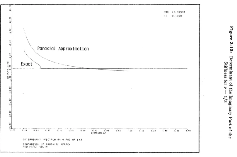
To investigate the energy-absorbing characteristics of the paraxial approximation, we again examine the determinant of the imaginary part of the stiffness matrix. The determinant of the imaginary parts of the true and the approximate in-plane stiffnesses are plotted in Figure 3-11 for

V = 4, and in Figure 3-12 for v = 3. The behavior of these curves is similar to that of the anti-plane case. The determinant of the true stiffness is positive until X2 = a2, the value of X at which the vertical wavenumber becomes imaginary, and is zero thereafter. The determinant of the paraxial approximation is positive in this range (following the shape of the true curve) and remains close to zero for X2 > a2.

Finally, Clayton and Engquist (1977) plot the dispersion relation for the paraxial approximation along with the true dispersion relation. Again, the parabloic curves of the approximation match the circles of the dispersion relation best when kX is small.

(49)

ROOTS OF THE IN-PLANE STIFFNESS MATRIX ROOT LAMBDA*"'2 1.40. 1.20. 1.00. 0.90. 0.60 0.40 0.20. 0.00 -0.20. -0.40

-0.01

-0.900

-1.00. -1.20] -1.40. - - AFROXIM EXACT ,6 >0 0 O) rj 0.05 0.10 0.15 0.20 0.25 0.30 0.35 0.40 0.45 0.50 POISSON MODLLUS