HAL Id: hal-00318327
https://hal.archives-ouvertes.fr/hal-00318327
Submitted on 4 Jun 2007
HAL is a multi-disciplinary open access
archive for the deposit and dissemination of
sci-entific research documents, whether they are
pub-lished or not. The documents may come from
teaching and research institutions in France or
abroad, or from public or private research centers.
L’archive ouverte pluridisciplinaire HAL, est
destinée au dépôt et à la diffusion de documents
scientifiques de niveau recherche, publiés ou non,
émanant des établissements d’enseignement et de
recherche français ou étrangers, des laboratoires
publics ou privés.
in Saturn’s ionosphere, and its relation to the UV
auroral oval observed by the Hubble Space Telescope
E. S. Belenkaya, I. I. Alexeev, M. S. Blokhina, S. W. H. Cowley, S. V.
Badman, V. V. Kalegaev, M. S. Grigoryan
To cite this version:
E. S. Belenkaya, I. I. Alexeev, M. S. Blokhina, S. W. H. Cowley, S. V. Badman, et al.. IMF dependence
of the open-closed field line boundary in Saturn’s ionosphere, and its relation to the UV auroral oval
observed by the Hubble Space Telescope. Annales Geophysicae, European Geosciences Union, 2007,
25 (5), pp.1215-1226. �hal-00318327�
www.ann-geophys.net/25/1215/2007/ © European Geosciences Union 2007
Annales
Geophysicae
IMF dependence of the open-closed field line boundary in Saturn’s
ionosphere, and its relation to the UV auroral oval observed by the
Hubble Space Telescope
E. S. Belenkaya1, I. I. Alexeev1, M. S. Blokhina1, S. W. H. Cowley2, S. V. Badman2, V. V. Kalegaev1, and M. S. Grigoryan1
1Institute of Nuclear Physics, Moscow State University, Vorob’evy Gory, 119992 Moscow, Russia 2Department of Physics & Astronomy, University of Leicester, Leicester LE1 7RH, UK
Received: 27 December 2006 – Revised: 30 April 2007 – Accepted: 7 May 2007 – Published: 4 June 2007
Abstract. We study the dependence of Saturn’s
magneto-spheric magnetic field structure on the interplanetary mag-netic field (IMF), together with the corresponding variations of the open-closed field line boundary in the ionosphere. Specifically we investigate the interval from 8 to 30 Jan-uary 2004, when UV images of Saturn’s southern aurora were obtained by the Hubble Space Telescope (HST), and simultaneous interplanetary measurements were provided by the Cassini spacecraft located near the ecliptic ∼0.2 AU up-stream of Saturn and ∼0.5 AU off the planet-Sun line to-wards dawn. Using the paraboloid model of Saturn’s mag-netosphere, we calculate the magnetospheric magnetic field structure for several values of the IMF vector representative of interplanetary compression regions. Variations in the mag-netic structure lead to different shapes and areas of the open field line region in the ionosphere. Comparison with the HST auroral images shows that the area of the computed open flux region is generally comparable to that enclosed by the auro-ral oval, and sometimes agrees in detail with its poleward boundary, though more typically being displaced by a few degrees in the tailward direction.
Keywords. Magnetospheric physics (auroral phenomena;
magnetospheric configuration and dynamics; planetary mag-netospheres; solar wind-magnetosphere interactions)
1 Introduction
The first unambiguous detections of polar ultraviolet (UV) auroras at Saturn were made by the Voyager spacecraft in 1980 and 1981 (e.g. Sandel and Broadfoot, 1981), and were later followed by observations from the Hubble Space Tele-scope (HST) (G´erard et al., 1995; Trauger et al., 1998). More recent HST observations of higher spatial resolution have
Correspondence to: E. S. Belenkaya
(elena@dec1.sinp.msu.ru)
shown that they generally form a ring around each pole ∼1◦–
3◦ thick, located between ∼10◦–20◦ co-latitude (e.g. Cow-ley et al., 2004a; G´erard et al., 2004; Badman et al., 2006). Such auroral rings can generally be formed either by the so-lar wind interaction, leading to emissions in the vicinity of the boundary between open and closed field lines, or by the current system associated with the maintenance of magneto-spheric plasma corotation deeper within the magnetosphere (e.g. Cowley and Bunce, 2001; Hill, 2001). From an anal-ysis of the latter current system, Cowley and Bunce (2003) concluded that the corotation-enforcement currents at Saturn are too weak and occur at too low a latitude to explain the observed UV auroras, and thus suggested that a solar wind-related origin was the more likely. These results have subse-quently been amplified by further modelling work presented by Cowley et al. (2004b), and also by the statistical analy-sis of the location of the UV auroras presented by Badman et al. (2006), who showed that they occur well poleward of the latitude where the magnetospheric plasma departs from near-rigid corotation according to Voyager data.
Direct evidence of the strong connection between Saturn’s UV auroras and the solar wind was first obtained during the joint HST-Cassini campaign in January 2004, when the Cassini spacecraft was upstream of the planet, en route to Saturn orbit insertion (Clarke et al., 2005; Crary et al. 2005; Bunce et al., 2006). Jackman et al. (2004) had shown that the interplanetary medium at the time of the Cassini approach, corresponding to the declining phase of the solar cycle, was strongly structured by corotating interaction regions (CIRs) into a recurrent pattern of high-field compression regions and low-field rarefaction regions. During the few-day compres-sion regions the interplanetary magnetic field (IMF) strength was typically 0.5–2 nT, while during the several day rarefac-tion intervals it was ∼0.1 nT or less. This structuring is ev-ident in Fig. 1, where we show the Cassini field and plasma data covering the interval of the HST observations, taken from Badman et al. (2005). The field data were obtained
Fig. 1. Stacked plot of Cassini IMF and plasma data obtained dur-ing the January 2004 Cassini-HST campaign. The first four panels
show the RTN magnetic field components (BR, BT, BN), and the
magnetic field magnitude |B| in nT. The fifth to seventh panels show
the solar wind proton velocity vsw (km s−1), the solar wind
den-sity np(cm−3), and the dynamic pressure Psw(nPa), respectively.
The bottom panel shows the estimated magnetopause reconnection voltage V (kV) using the algorithm of Jackman et al. (2004). The dashed vertical lines indicate the corresponding times of the HST images shown in Fig. 2, adjusted to take into account the solar wind propagation delay and the Saturn-HST light propagation delay (fig-ure adapted from Badman et al., 2005).
by the Cassini magnetic field investigation (Dougherty et al., 2004), and are shown in RTN coordinates. RTN is a right-handed spherical polar system referenced to the Sun’s spin axis, with BR directed radially outward from the Sun,
BT azimuthal in the direction of planetary motion around the
Sun, and BN normal to the other two components, positive
northward from the equatorial plane. The plasma parameters were derived from Cassini CAPS particle spectrometer data (Young et al., 2004). The times of the HST imaging intervals are shown by the vertical dashed lines, where account has been taken of the ∼17 h solar wind radial propagation delay from Cassini to Saturn, and of the 68-min light travel time
from Saturn to the HST. The solar wind delay is uncertain to within a few hours, however, due to possible non-radial propagation effects and the difference in the heliocentric lon-gitude of Cassini and Saturn (Crary et al., 2005). During this interval Cassini was located near the ecliptic ∼0.2 AU up-stream of Saturn, and ∼0.5 AU off the Sun-planet line toward dawn.
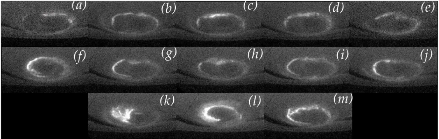
It can be seen that the HST observations encompass two rarefaction regions, the earlier one being somewhat “deeper” than the later, together with two compression re-gions bounded by interplanetary shocks. The first “minor” compression onset occurred on 16 January, while the sec-ond “major” compression onset occurred on 26 January. The auroral observations themselves are shown in Fig. 2, letter coded as in Fig. 1 (Clarke et al., 2005; Bunce et al., 2006). These show the Southern Hemisphere of the planet with the noon meridian toward the top of each image, dawn to the left, and dusk to the right. It can be seen that the auroral distributions observed after the compression onsets in im-ages (f) and (k) (at intervals of ∼40 and ∼11 h after the ini-tial shock, respectively) show contracted brightened ovals, with the whole of the dawn-side polar cap being filled with bright sun-aligned arcs in the latter case. Thus, although the strength of the IMF at Saturn’s orbit is typically an order of magnitude less than that at Earth, and the dynamic pres-sure typically two orders of magnitude less, the interaction with the interplanetary medium nevertheless remains impor-tant for Saturn’s magnetosphere.
Badman et al. (2005) investigated the variations in the amount of magnetic flux contained within the “dark” region poleward of Saturn’s auroras in the January 2004 data shown in Fig. 2, and found that it varied between ∼15 to ∼50 GWb, with the smallest values being associated with the intervals following compression onsets. On the assumption that the poleward boundary of the auroras represents an approximate proxy for the open-closed field line boundary, in accordance with the above discussion, it was thus inferred that major open flux closure events were triggered by these interplan-etary events, with the open flux then increasing again in the subsequent few-day high-field intervals. Belenkaya et al. (2006a) have also studied these data, and in addition to the compression-induced flux closure just mentioned, have also discussed the role of a three-dimensional current system in the auroral dynamics, arising from the solar wind interaction. This current system includes Region 1 field-aligned currents (FACs) concentrated at the open-closed field line boundary, “SBZ” FACs distributed over the polar cap near the cusp for southward IMF (the kronian counterpart of “NBZ” currents at Earth arising under northward IMF conditions), together with the Pedersen currents on open field lines in the iono-sphere which close both these systems. The Region 1 cur-rents are added to the ring of upward FAC of comparable magnitude at the boundary of open field lines which is as-sociated with differential plasma rotation between open and closed field lines, such that the overall current system for the
(a)
(b)
(c)
(d)
(e)
(f)
(g)
(h)
(i)
(j)
(k)
(l)
(m)
Fig. 2. UV images of Saturn’s southern aurora obtained by HST-STIS on 8, 10, 12, 14, 16, 18, 20, 21, 23, 24, 26, 28, and 30 January 2004 (panels a to m, respectively). The panels have been generated by combining individual images obtained on a given HST orbit (Clarke et al., 2005; Bunce et al., 2006). The noon meridian is at the centre top of each plot, with dawn to the left (figure from Bunce et al., 2006).
January 2004 events takes the form of strong upward FAC on the dawn side, with corresponding bright aurora, and weaker upward (or even downward) FAC at dusk, with weaker (or absent) auroras. Figure 2 shows that such dawn-dusk asym-metry is characteristic of the bright active intervals observed in January 2004.
In this paper we investigate IMF influences on the size and position of the open field region at Saturn during these ac-tive intervals, corresponding to periods when the interplane-tary field was at its strongest, such that the IMF effects may be most evident. Our calculations are based on the Saturn magnetospheric model described by Alexeev et al. (2006) and Belenkaya et al. (2006b), in which the magnetopause is taken to be a paraboloid of revolution about the Saturn-Sun line. Kronian solar-magnetospheric coordinates (KSM) are thus employed, in which the X-axis is directed towards the Sun, Saturn’s magnetic moment Ms lies in the X-Z plane,
and Y completes the right-handed orthogonal triad. It may be noted that for the January 2004 interval the difference between KSM and the heliospheric RTN system employed in Fig. 1 is very small, such that Bx≈–BR, By≈–BT, and
Bz≈BN. The main contributors to the model magnetic field
are then (i) the intrinsic magnetic (dipole) field of the planet, as well as the shielding magnetopause current which confines the dipole field inside the magnetopause, (ii) the ring current and the shielding magnetopause current that similarly con-fines its field inside the magnetopause, (iii) the tail currents and their magnetopause closure currents, and (iv) the IMF which penetrates into the magnetosphere. We note that the principal interplanetary influences on the model derive from the solar wind dynamic pressure which determines the posi-tion of the magnetopause and hence the overall size of the system, and the direction and strength of the interplanetary field which is reflected in the penetrating IMF component. We also note that the ring current is modelled as a thin
equa-torial disc in which the azimuthal current intensity falls as the inverse square of the radial distance, and that the tail current is re-scaled from an earlier terrestrial model.
The parameters which define Saturn’s magnetospheric magnetic field in the model are thus as follows: (i) Rss is
the distance from Saturn’s centre to the subsolar point on the magnetopause; (ii) Rrc1and Rrc2are the distances to the
outer and inner edges of the ring current, respectively; (iii) R2is the distance from the planet’s centre to the inner edge
of the magnetospheric tail current sheet; (iv) the field mag-nitude of the tail currents at the inner edge of the tail current sheet is Bt/α0, where α0=(1+2R2/Rss)1/2; (v) 9 is the tilt
angle between the magnetic dipole direction and the KSM Z axis (∼25◦during the January 2004 interval, correspond-ing to Northern Hemisphere winter conditions); (vi) Brc1is
the radial component of the ring current magnetic field at the outer edge of the ring current; (vii) the effect of the IMF in-side the magnetosphere is given by the uniform field ksBIMF,
where BIMF is the IMF vector and kS is the coefficient of
its penetration into the magnetosphere. With regard to the latter model assumption, we note that Alexeev (1986) ob-tained a finite-conductivity solution for the magnetic field in the magnetosheath, in which magnetic field diffusion results in only a partial screening of the IMF by the magnetopause. The magnetic field inside the magnetosphere was then found to be some fraction kS of the external field, depending on
the value of the magnetic Reynolds number Rm. In the next
section we calculate the size and location of the open flux region in Saturn’s ionosphere using this model, employing parameter values determined by Belenkaya et al. (2006b) ap-propriate for compressed active conditions.
2 Paraboloid model calculations for the cases of 16 and 26 January 2004
As can be seen in Fig. 1, during the “minor” compres-sion region occurring between 16 and 18 January, the KSM components of the IMF can be characterised by (Bx, By, Bz)=(0.0, −0.4, −0.4) nT (Belenkaya et al., 2006a).
These values are taken as characteristic of the interval sur-rounding the maximum in pressure during the “minor” com-pression, near the “shifted” time of image (f). The solar wind density increased to 0.1 cm−3, while the speed also increased to ∼530 km s−1. Following this compression, a rarefaction region was then observed between days 19 and 25, with an IMF field strength ∼0.3 nT, a density of 0.01– 0.04 cm−3, and with almost the same solar wind speed. The “major” compression then occurred on 25 January, and lasted essentially to the end of the interval considered. During this compression the IMF strength was ∼1–2 nT, the den-sity increased to ∼0.03–0.1 cm−3, and the solar wind speed increased to ∼630 km s−1. Belenkaya et al. (2006a) esti-mated that during the earlier part of this event the KSM IMF components were approximately (0.5, −2.0, −1.4) nT. These values correspond to the interval near the time of im-age (k), just prior to the pressure maximum during the com-pression event. Later in the event, near the time of image (m), the IMF can reasonably be typified by KSM components (−0.3, 0.7, 0.7) nT. In our calculations below we use the three IMF values given here as representative of the two compres-sion intervals, together with other model parameters intended to reflect the compressed magnetospheric conditions then prevailing. Specifically, we employ the values determined by Belenkaya et al. (2006b) appropriate to the compressed magnetosphere observed during the Pioneer-11 flyby, given by Rss=17.5 RS, Rrc1=12.5 RS, Rrc2=6.5 RS, R2=14 RS,
Bt=8.7 nT, and Brc1=3.62 nT, where RS=60 330 km is the
equatorial value of Saturn’s radius. These values should therefore also provide a reasonable representation for the compressed conditions of interest here, given that the results should not be sensitively dependent on the exact choices.
With regard to the value of the IMF penetration parameter kS, we note that Belenkaya (2006a) used values of 0.2 and
0.8 for rough estimations. Earlier, Belenkaya (2004) showed that the value 0.8 was most appropriate at Jupiter for the in-terpretation of observations of anti-corotational solar wind-driven plasma flow in the equatorial magnetosphere. Tsy-ganenko (2002) found that the best correspondence between his model of the near-Earth magnetosphere and observational data was obtained for an IMF penetration coefficient between 0.15 and 0.8. The larger size of Saturn’s magnetosphere com-pared to Earth (by a factor of ∼16) is expected to decrease kS
by a factor of ∼2, since kS is proportional to Rm−1/4and Rm
is proportional to the size of the magnetosphere. However, as deduced by Alexeev et al. (2003), plasma compression at the bow shock increases kSby a factor of ∼2, and a high level of
magnetic field variability in Saturn’s magnetosheath can also
lead to an increase in kS. Overall, we thus expect that kS for
Saturn should be similar to or larger than that for Earth. Here we will therefore consider values of kS within the range 0.2
to 0.8.
In Fig. 3 we present some results illustrating Saturn’s mag-netic field lines for the above model parameters, together with kS=0.8 and KSM IMF vectors given from top to
bot-tom of the figure by (0.0, −0.4, −0.4), (0.5, −2.0, −1.4), and (−0.3, 0.7, 0.7) nT. The first two are the southward-directed IMF vectors corresponding to the above “minor” and initial “major” compression regions, while the third is the northward-directed field corresponding to the later part of the “major” compression. The field lines shown start from the ionosphere on the noon and midnight meridians, but, due to the presence of the IMF By component, are twisted out
of the meridian in the region away from the planet. In the left-hand column of Fig. 3 we show the projection of these field lines on the X-Z plane, while in the right-hand column we provide an indication of the 3-D structure. In the up-per two panels with southward IMF we see that the size of the modelled region of field lines having even one “end” in the ionosphere (open and closed), decreases as the IMF field strength increases. The bottom panel shows that the structure of the model magnetic field lines changes dramatically when the IMF becomes northward-directed.
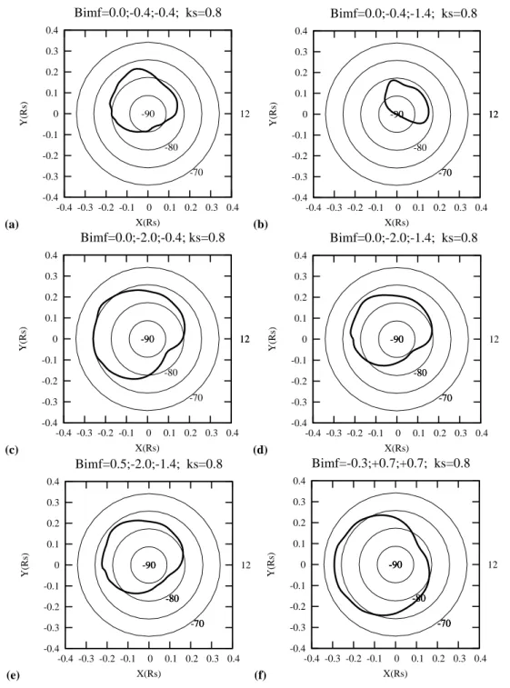
In Fig. 4 we correspondingly show how the open-closed field line boundary varies in response to the IMF vec-tor, specifically for the Southern Hemisphere, thus match-ing the auroral images shown in Fig. 2. The view is looking “through” the planet onto the southern pole, with noon on the right side of these figures, and dusk at the top. Panel (a) corresponds to the “minor” compression on 16 January with KSM vector (0.0, −0.4, −0.4) nT (and 9=25.05◦). The open field region is displaced to the dusk side of the pole due to the presence of the IMF By
compo-nent. In panel (b) the northward Bzcomponent has been
in-creased in magnitude to −1.4 nT, such that the KSM com-ponents are (0.0, −0.4, −1.4) nT. The open field region shrinks and becomes centred sunward as well as duskward of the pole. Panel (c) shows how the open area responds to the By field, with an IMF given by KSM components
(0.0, −2.0, −0.4) nT. In this case the open region becomes enlarged in area. In panel (d) we then increase the magni-tude of the northward field component again to −1.4 nT, so that the KSM components become (0.0, −2.0, −1.4) nT. The increased magnitude of the southward-directed field again re-sults in a decrease in the open area. Panel (e) then shows the effect of changing the Bx component, with an IMF vector
of (0.5, −2.0, −1.4) nT, which thus now corresponds to the “major” compression region on 26 January (with 9=24.64◦). The open field region is almost unchanged compared with panel (d) in this case. Finally, in panel (f) we show results for the northward-directed IMF given by (−0.3, 0.7, 0.7) nT, corresponding to the later part of the “major” compression. In this case the open field line region significantly increases
-60 -40 -20 0 20 40 60 -200 -150 -100 -50 0 50 Z(Rs) X(Rs) Bimf=0.0;-0.4;-0.4; ks=0.8 -60 -40 -20 0 20 40 60 -200 -150 -100 -50 0 50 Z(Rs) X(Rs) Bimf=0.5;-2.0;-1.4; ks=0.8 -60 -40 -20 0 20 40 60 -200 -150 -100 -50 0 50 Z(Rs) X(Rs) Bimf=-0.3;0.7;0.7; ks=0.8 Bimf=0.0;-0.4;-0.4; ks=0.8 -200 -150 -100 -50 0 50 X(Rs) -100-80 -60-40 -20 0 20 40 Y(Rs) -60 -40 -20 0 20 40 60 Z(Rs) Bimf=0.5;-2.0;-1.4; ks=0.8 -200 -150 -100 -50 0 50 X(Rs) -60-40 -20 0 20 40 60 Y(Rs) -60 -40 -20 0 20 40 60 Z(Rs) Bimf=-0.3;0.7;0.7; ks=0.8 -200 -150 -100 -50 0 50 X(Rs) -100-80 -60-40 -20 0 20 40 Y(Rs) -60 -40 -20 0 20 40 60 Z(Rs)
Fig. 3. Plots showing the field lines emerging from Saturn’s ionosphere in the noon and midnight meridians. On the left-hand side of the plot the field lines are projected into the X-Z plane, while the 3-D structure is indicated on the right-hand side. The three rows correspond to dif-fering IMF vectors. From top to bottom these are given by KSM components of (0.0, −0.4, −0.4), (0.5, −2.0, −1.4), and (−0.3, 0.7, 0.7) nT, corresponding to the “minor” field compression interval, and the initial and later “major” compression intervals, respectively. The input
model parameters are Rss=17.5 RS, R2=14 RS, Rrc1=12.5 RS, Rrc2=6.5 RS, Brc1=3.6 nT, Bt=−8.7 nT, and kS=0.8. The dipole tilt angle is
(a) -0.4 -0.3 -0.2 -0.1 0 0.1 0.2 0.3 0.4 -0.4 -0.3 -0.2 -0.1 0 0.1 0.2 0.3 0.4 Y(Rs) X(Rs) Bimf=0.0;-0.4;-0.4; ks=0.8 -80 -70 12 -90 (b) -0.4 -0.3 -0.2 -0.1 0 0.1 0.2 0.3 0.4 -0.4 -0.3 -0.2 -0.1 0 0.1 0.2 0.3 0.4 Y(Rs) X(Rs) -90 Bimf=0.0;-0.4;-1.4; ks=0.8 -70 12 -90 -80 -70 12 (c) -0.4 -0.3 -0.2 -0.1 0 0.1 0.2 0.3 0.4 -0.4 -0.3 -0.2 -0.1 0 0.1 0.2 0.3 0.4 Y(Rs) X(Rs) -90 Bimf=0.0;-2.0;-0.4; ks=0.8 12 -90 -80 -70 12 (d) -0.4 -0.3 -0.2 -0.1 0 0.1 0.2 0.3 0.4 -0.4 -0.3 -0.2 -0.1 0 0.1 0.2 0.3 0.4 Y(Rs) X(Rs) -90 -90 -80 Bimf=0.0;-2.0;-1.4; ks=0.8 -90 -80 -70 12 -70 (e) -0.4 -0.3 -0.2 -0.1 0 0.1 0.2 0.3 0.4 -0.4 -0.3 -0.2 -0.1 0 0.1 0.2 0.3 0.4 Y(Rs) X(Rs) -90 -90 -80 -90 Bimf=0.5;-2.0;-1.4; ks=0.8 -80 -70 12 -70 -80 -70 (f) -0.4 -0.3 -0.2 -0.1 0 0.1 0.2 0.3 0.4 -0.4 -0.3 -0.2 -0.1 0 0.1 0.2 0.3 0.4 Y(Rs) X(Rs) -90 -90 -80 -90 -90 Bimf=-0.3;+0.7;+0.7; ks=0.8 -70 12 -70 -80 -70 -80 -70
Fig. 4. Open field line regions in Saturn’s southern ionosphere calculated using the paraboloid model for various sets of IMF components. In panels (a–f) the KSM components are as follows: (a) (0.0, −0.4, −0.4) nT, (b) (0.0, −0.4, −1.4) nT, (c) (0.0, −2.0, −0.4) nT, (d) (0.0, −2.0, −1.4) nT, (e) (0.5, −2.0, −1.4) nT, and (f) (−0.3, 0.7, 0.7) nT. The view is looking “through” the planet onto the southern pole,
with noon at the right, dusk at the top, and co-latitude is indicated at intervals of 5◦. The model parameters are as in Fig. 3.
in size.
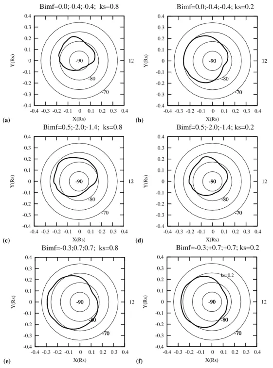
In Fig. 5 we also show how the open field line region varies with the value of the IMF penetration coefficient kS, again for
the Southern Hemisphere. On the left-hand side of the figure we reproduce the results shown in Fig. 4 which correspond to the typical IMF conditions during the “minor” and initial
and later “major” compression intervals using kS=0.8
(pan-els a, e, and f in Fig. 4, respectively). On the right-hand side we show results for the same IMF vector, but with kS=0.2.
We see that the value of kS smoothly changes the open field
line area in the ionosphere. At the same time, the value of kS significantly influences the polar cap potential drop and
(a) -0.4 -0.3 -0.2 -0.1 0 0.1 0.2 0.3 0.4 -0.4 -0.3 -0.2 -0.1 0 0.1 0.2 0.3 0.4 Y(Rs) X(Rs) Bimf=0.0;-0.4;-0.4; ks=0.8 -80 -70 12 -90 (b) -0.4 -0.3 -0.2 -0.1 0 0.1 0.2 0.3 0.4 -0.4 -0.3 -0.2 -0.1 0 0.1 0.2 0.3 0.4 Y(Rs) X(Rs) -90 Bimf=0.0;-0.4;-0.4; ks=0.2 -70 12 -90 -80 -70 12 (c) -0.4 -0.3 -0.2 -0.1 0 0.1 0.2 0.3 0.4 -0.4 -0.3 -0.2 -0.1 0 0.1 0.2 0.3 0.4 Y(Rs) X(Rs) -90 Bimf=0.5;-2.0;-1.4; ks=0.8 12 -90 -80 -70 12 (d) -0.4 -0.3 -0.2 -0.1 0 0.1 0.2 0.3 0.4 -0.4 -0.3 -0.2 -0.1 0 0.1 0.2 0.3 0.4 Y(Rs) X(Rs) -90 -90 -80 Bimf=0.5;-2.0;-1.4; ks=0.2 -90 -80 -70 12 -70 (e) -0.4 -0.3 -0.2 -0.1 0 0.1 0.2 0.3 0.4 -0.4 -0.3 -0.2 -0.1 0 0.1 0.2 0.3 0.4 Y(Rs) X(Rs) -90 -90 -80 -90 Bimf=-0.3;0.7;0.7; ks=0.8 -80 -70 12 -70 -80 -70 (f) -0.4 -0.3 -0.2 -0.1 0 0.1 0.2 0.3 0.4 -0.4 -0.3 -0.2 -0.1 0 0.1 0.2 0.3 0.4 Y(Rs) X(Rs) -90 -90 -80 -90 -90 Bimf=-0.3;+0.7;+0.7; ks=0.2 -70 12 -70 -80 -70 -80 -70 ks=0.2
Fig. 5. As for Fig. 4, but showing how the open field area varies with the IMF penetration parameter kS. The panels on the left side reproduce
those shown in panels (a), (e), and (f) of Fig. 4 with kS=0.8, while those shown on the right side have the same IMF vector, but now with
kS=0.2.
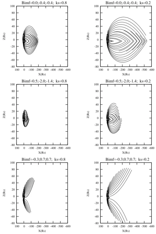
the global magnetospheric magnetic field structure, as can be seen in Fig. 6. This figure shows the magnetospheric field lines for these cases projected onto the X-Z plane in the same format as the left-hand panels of Fig. 3. It can be seen that the global size of the modelled region of Saturn’s open and closed magnetospheric field lines depends strongly on the
kS value. It should be realised that, although the bounding
paraboloid magnetopause is of fixed size in Figs. 3 and 6, considerable volumes in the model “tail” region contain field lines that do not connect with the planet at either end (e.g. Belenkaya, 1998), and are consequently not shown in these figures.
-80 -60 -40 -20 0 20 40 60 80 100 -600 -500 -400 -300 -200 -100 0 100 Z(Rs) X(Rs) Bimf=0.0;-0.4;-0.4; ks=0.8 -80 -60 -40 -20 0 20 40 60 80 100 -600 -500 -400 -300 -200 -100 0 100 Z(Rs) X(Rs) Bimf=0.0;-0.4;-0.4; ks=0.2 -80 -60 -40 -20 0 20 40 60 80 100 -600 -500 -400 -300 -200 -100 0 100 Z(Rs) X(Rs) Bimf=0.5;-2.0;-1.4; ks=0.8 -80 -60 -40 -20 0 20 40 60 80 100 -600 -500 -400 -300 -200 -100 0 100 Z(Rs) X(Rs) Bimf=0.5;-2.0;-1.4; ks=0.2 -80 -60 -40 -20 0 20 40 60 80 100 -600 -500 -400 -300 -200 -100 0 100 Z(Rs) X(Rs) Bimf=-0.3;0.7;0.7; ks=0.8 -80 -60 -40 -20 0 20 40 60 80 100 -600 -500 -400 -300 -200 -100 0 100 Z(Rs) X(Rs) Bimf=-0.3;0.7;0.7; ks=0.2
Fig. 6. Plots of magnetospheric field lines projected into the X-Z plane in the same format as the left side of Fig. 3, but now for IMF vectors and penetration coefficients corresponding to the six panels of Fig. 5.
Alexeev et al. (1998) previously showed that even in the case when the model magnetosphere is “closed” (e.g. with kS=0 or with no IMF), the model contains long tail
lobe magnetic field lines which are directed almost parallel to the equatorial plane, and intersect the distant tail cross section perpendicular to the x-axis. These open field lines
may be considered to be formed from previous interactions between the magnetosphere and the interplanetary medium, and may thus be taken to correspond, for example, to the open flux which is present during “deep” rarefaction regions when the IMF is very weak. Alexeev et al. (2006) estimated the open flux in each tail lobe in terms of the
model parameters as 80=(π /2)(1+2R2/Rss)BtR2ss (see also
Belenkaya et al., 2006b). This represents the “baseline” open flux that is present for the model for kS=0. For
the chosen magnetospheric input parameters employed here (Rss=17.5 RS, R2=14 RS, Bt=8.7 nT) we obtain
80=7529.5 nT RS2 (27.4 GWb). We can readily estimate
the ionospheric co-latitude corresponding to this amount of magnetic flux. The dipole magnetic field strength at Saturn’s equator is BS0=21 160 nT, so that the magnetic field strength
at the pole is roughly Bp=2BS0=42 320 nT. The flux 80can
also be written as BpS0, where S0is the area of the open field
line region in the ionosphere for the “baseline” model, and S0=π ρ2, where ρ is the radius of this region, and ρ=RSsinθ ,
where θ is the co-latitude of the open-closed field line boundary. Thus, 80=Bpπ RS2 sin2θ , and correspondingly
sinθ =(80/(Bpπ R2S))1/2=(7529.5 nT R2S/(42 320 nT π R2S))1/2
=0.24, thus θ ∼14◦. This value may be considered to provide a rough estimation of the effective open field line region boundary co-latitude for the “baseline” model with kS=0.
It is well known for the case of the Earth that the radius of the region of open field lines depends on the north-south component of the IMF. The experimental evidence is sum-marized, for example, by Holzworth and Meng (1984) and Bolshakova et al. (1988), while the dependence in numerical models was obtained, for example, by Alexeev et al. (1993) and Belenkaya (1998). For the Earth the open field line re-gion increases for southward IMF, and decreases for north-ward IMF, which is the opposite for Saturn, due to the oppo-site sense of the planetary magnetic moment. The situation which most closely represents the “baseline” case in those computed here is Fig. 5f for a weak northward IMF. We see that for this case the boundary is located at ∼12.5◦, which is in reasonable accord with the rough (14◦) estimation above, based on the open tail lobe flux. We also note that Alexeev (2005) gave a relation which determines the size of the po-lar cap for the “ground state” of the Earth’s magnetosphere. Recasting Alexeev’s (2005) Eq. (6) for the case of Saturn’s magnetosphere, we find sinθ =(2.2 RS/3 RSS)1/2=0.2, which
gives θ =11.8◦. The difference of 0.7◦between this value of the polar cap size and that shown in Fig. 5f may be due to the weak northward IMF, or physically to small magnetospheric disturbances. Both factors increase the amount of open flux in the magnetosphere. The same factors may also explain the modestly increased flux in our kS=0 “baseline” Saturn model
compared with Alexeev’s (2005) estimation. We finally note that the “baseline” model should also provide an initial de-scription of magnetic field conditions during “deep” rarefac-tion regions when the IMF is very weak. However, this is not a matter we explore in detail here, concentrating instead on conditions during solar wind compressions.
3 Comparison with auroral observations
We now compare the results shown in Figs. 4 and 5 with the observed auroral distributions shown in Fig. 2, which corre-spond to the interplanetary data shown in Fig. 1, as indicated by the vertical dashed lines (within the few-hour uncertain-ties of the latter’s timing). As discussed previously by Bad-man et al. (2005) and Bunce et al. (2006), the first HST ob-servations during the 2004 Cassini campaign, on 8 January, were obtained during a “deep” rarefaction region. The cor-responding auroral oval (image a) was highly expanded at 15◦–20◦co-latitude, with brightenings observed in the pre-midnight, dawn, and pre-noon sector. By 15 January (im-age e) the open field line region radius was a little smaller, around 12◦–18◦. After the arrival of the “minor” solar wind
compression at Saturn (on 16 January), the radius of the con-tracted open field line region varied from 5◦–8◦in the
post-midnight and dawn sectors to ∼13◦in the post-noon sector, with the brightness decreasing from post-midnight anticlock-wise into the pre-midnight hours. During the subsequent “in-termediate” rarefaction region, a re-expanded oval was seen on 23 January (image i) with auroral brightenings at dawn and noon. On 26 January, at the onset of the “major” CIR compression, a highly brightened and contracted oval was observed (image k), with bright auroral forms on the dawn-side from ∼3◦to ∼15◦co-latitude. On 30 January, near the end of the “major” compression, bright auroras were still ob-served except in the pre-midnight sector (image m), and the oval re-expanded to 12◦–15◦co-latitude in the pdawn re-gion.
We now more directly compare the calculated open field line areas shown in Fig. 5 with the corresponding compres-sion region auroral images shown in Fig. 2. In Fig. 7 pan-els (a–c) we thus show images (f), (k), and (m), respectively, projected onto a polar grid in which the southern ionosphere is viewed “through” the planet from the north, as in Figs. 4 and 5, with noon now at the bottom of each plot, and dawn to the left. The dotted circles are at intervals of 10◦co-latitude, and the auroral intensities are indicated by the colour scale shown on the right. Smoothed calculated open field bound-aries are then over-plotted on the images, where the solid lines correspond to kS=0.2 (Figs. 5b, d, and f in (a), (b), and
(c) respectively), and the dashed lines to kS=0.8 (similarly
Figs. 5a, c, and e). Some important points emerge from these comparisons. First, the size of the calculated area of open flux generally agrees very well with the area encircled by the UV auroras, within the limitations imposed by the continuity of the observed auroral emission in local time. The bound-aries for the two kS values are essentially indistinguishable
in panels (b) and (c), while in panel (a) the larger area for kS=0.2 agrees better with the area poleward of the emissions
than does the smaller area for kS=0.8. These results thus
pro-vide support for the hypothesis made by Badman et al. (2005) that the dark area poleward of the auroral emission corre-sponds to open field lines. Second, with regard to the detailed
Fig. 7. UV images of Saturn’s southern polar aurora obtained during January 2004 are shown projected onto a polar grid, from the pole to
30◦co-latitude, again viewed as though looking “through” the planet onto the southern pole, as in Figs. 4 and 5. However, noon is now at
the bottom of each plot and dawn to the left, as indicated. The UV auroral intensity is colour-coded according to the scale shown on the right-hand side of the figure. Panels (a–c) show images (f), (k), and (m) in Fig. 2, respectively, whose HST start times are given at the top of each plot. These projected images are reproduced from Badman et al. (2005). The over-plotted solid and dashed white lines show the
smoothed calculated locations of the boundary of open field lines for kS=0.2 and 0.8, respectively. The curves in panel (a) thus correspond
to Figs. 5a and b, respectively, those in panel (b) to Figs. 5c and d, and those in panel (c) to Figs. 5e and f.
Fig. 8. Comparison of the computed Southern Hemisphere open
field regions for kS=0.8 shown in panels (a), (c), and (e) of Fig. 5
(and a, e, and f of Fig. 4), shown by the green, blue, and purple lines, respectively, with the median poleward (yellow stars) and equator-ward (red crosses) southern auroral boundary locations determined by Badman et al. (2006) (their Fig. 5). The plot format is the same
as for Figs. 4 and 5. The red lines show co-latitude circles at 5◦
intervals from the southern pole to −70◦.
position of the calculated open field region relative to the au-roras, it can be seen that this agrees very well with the pole-ward boundary of the auroras in panel (c) (for which the IMF is northward). In panel (b) (for which the IMF is southward), the bright dawn auroras also lie at and just inside the calcu-lated open field boundary in this local time sector. Finally, in panel (a) (for which the IMF is weakly southward) the calcu-lated boundary for kS=0.2 is of a similar size and shape as the
poleward boundary of the auroras, as just indicated, but the latter are displaced significantly toward noon, compared, for example, with the similar distribution shown in panel (c). For further discussion of the auroral distributions seen in these images and their relationship to solar wind-magnetosphere-ionosphere coupling current systems, the reader is referred to the results of Belenkaya et al. (2006a), discussed briefly in the Introduction.
We can also compare these calculated open field bound-aries with the typical position of the UV oval determined by Badman et al. (2006). These authors presented an analysis of a selection of twenty-two HST images of Saturn’s auro-ras obtained during 1997–2004, including the images shown here in Fig. 2. In Fig. 8 the yellow stars and red crosses show the median poleward and equatorward boundaries of the au-rora determined from these images, respectively, plotted on a polar grid in the same format as Figs. 4 and 5. The local time coverage ranges from the pre-dawn sector to post-dusk via noon. The green, blue, and purple curves then show the cal-culated open field boundaries for kS=0.8 shown in panels (a),
(c), and (e) of Fig. 5 (and a, e, and f of Fig. 4), respectively, thus corresponding to the “minor” compression region, the
initial “major” compression region, and the later “major” compression region, respectively, in the January 2004 data. It can be seen that all of these calculated boundaries lie a few degrees poleward of the median poleward auroral boundary in the noon sector, roughly intermediate between panels (a) and (c) in Fig. 7, while the largest boundary approaches the median oval in the dawn sector.
4 Conclusions
In this paper we have investigated the IMF-dependence of the open field line region in Saturn’s ionosphere using the paraboloid model of the magnetosphere, combined with IMF data obtained by the Cassini spacecraft during its approach to Saturn in January 2004. We have compared these results with simultaneous images of Saturn’s UV auroras obtained by the HST, specifically the bright active emissions observed during interplanetary compression regions when the IMF is strongest. It has been shown that the IMF direction signifi-cantly changes the magnetospheric magnetic field structure, together with the area and shape of the region of open field lines. Comparison with related auroral images shows that the calculated area of open field lines is comparable to that enclosed by the auroral oval, in support of previous hypothe-ses to this effect. In addition, the position of the calculated open field region sometimes agrees in detail with the pole-ward boundary of the auroral oval, though more typically being displaced by a few degrees of latitude in the tailward direction. We thus conclude on the basis of these results that the solar wind and its magnetic field plays a major role in the generation of Saturn’s auroras.
Acknowledgements. Work at the Institute of Nuclear Physics,
Moscow State University was supported by INTAS Grant No 03-51-3922 and by the RFBR Grants 05-05-64435, 06-05-64508, and 07-05-00529. Work at Leicester was supported by PPARC/STFC grants PPA/G/O/2003/00013 and PP/E000983/1. SWHC was sup-ported by a Royal Society Leverhulme Trust Senior Research
Fel-lowship. The auroral data from which Figs. 2, 7, and 8 have
been prepared are courtesy of J. Clarke (Boston University), and J.-C. G´erard and D. Grodent (Universit´e de Li`ege).
Topical Editor I. A. Daglis thanks J. Nichols and another referee for their help in evaluating this paper.
References
Alexeev, I. I.: The penetration of interplanetary magnetic and elec-tric fields into the magnetosphere, J. Geomagn. Geoelectr., 38, 1199–1221, 1986.
Alexeev, I. I., Belenkaya, E. S., Bobrovnikov, S. Yu., and Kale-gaev, V. V.: Modelling of the electromagnetic field in the in-terplanetary space and in the Earth’s magnetosphere, Space Sci. Rev., 107, 7–26, 2003.
Alexeev, I. I.: What defines the polar cap and auroral oval diam-eters?, in: The Inner Magnetosphere: Physics and Modeling,
edited by: Pulkkinen, T. I., Tsyganenko, N. A., and Friedel, R. H. W., Geophys. Mon. Ser., 155, 257–262, AGU, 2005. Alexeev, I. I., Belenkaya, E. S., and Sibeck, D. G.: Open field lines
in the closed model of the magnetosphere (in Russian), Geo-magn. Aeron., 38, 9–18, 1998.
Alexeev, I. I., Belenkaya, E. S., Kalegaev, V. V., and Lutov, Yu. G.: Electric fields and field-aligned current generation in the magne-tosphere, J. Geophys. Res., 98, 4041–4051, 1993.
Alexeev, I. I., Kalegaev, V. V., Belenkaya, E. S., Bobrovnikov, S. Y., Bunce, E. J., Cowley, S. W. H., and Nichols, J. D.: A global magnetic model of Saturn’s magnetosphere, and a com-parison with Cassini SOI data, Geophys. Res. Lett., 33, L08101, doi:10.1029/2006GL025896, 2006.
Badman, S. V., Bunce, E. J., Clarke, J. T., Cowley, S. W. H., G´erard, J.-C., Grodent, D., and Milan, S. E.: Open flux estimates in Saturn’s magnetosphere during the January 2004 Cassini-HST campaign, and implications for reconnection rates, J. Geo-phys. Res., 110, A11216, doi:10.1029/2005JA011240, 2005. Badman, S. V., Cowley, S. W. H., G´erard, J.-C., and Grodent, D.: A
statistical analysis of the location and width of Saturn’s southern auroras, Ann. Geophys., 24, 3533–3545, 2006,
http://www.ann-geophys.net/24/3533/2006/.
Belenkaya, E. S.: High-latitude ionospheric convection patterns de-pendent on the variable IMF orientation, J. Atmos. Solar-Terr. Phys., 60/13, 1343–1354, 1998.
Belenkaya, E. S.: The jovian magnetospheric magnetic and electric fields: Effects of the interplanetary magnetic field, Planet. Space Sci., 52, 499–511, 2004.
Belenkaya, E. S., Cowley, S .W. H., and Alexeev, I. I.: Saturn’s aurora in the January 2004 events, Ann. Geophys., 24, 1649– 1663, 2006a.
Belenkaya, E. S., Alexeev, I. I., Kalegaev, V. V., and Blokhina, M. S.: Definition of Saturn’s magnetospheric model parameters for the Pioneer 11 flyby, Ann. Geophys., 24, 1145–1156, 2006b. Bolshakova, O. V., Kleimenova, N. G., and Kurazhkovskaya, N. A.:
Polar cap dynamics on the observations of the long period ge-omagnetic pulsations (in Russian), Geomagn. Aeron., 28, 661– 665, 1988.
Bunce, E. J., Cowley, S. W. H., Jackman, C. M., Clarke, J. T., Crary, F. J., and Dougherty, M. K.: Cassini observations of the interplanetary medium upstream of Saturn and their relation to Hubble Space Telescope aurora data, Adv. Space Res., 38, 806– 814, 2006.
Clarke, J. T., G´erard, J.-G., Grodent, D., Wannawichian, S., Gustin, J., Connerney, J., Crary, F., Dougherty, M., Kurth, W., Cowley, S. W. H., Bunce, E. J., Hill, T., and Kim, J.: Morpholog-ical differences between Saturn’s ultraviolet aurorae and those of Earth and Jupiter, Nature, 433, 717–719, 2005.
Cowley, S. W. H. and Bunce, E. J.: Origin of the main auroral oval in Jupiter’s coupled magnetosphere-ionosphere system, Planet. Space Sci., 49, 1067–1088, 2001.
Cowley, S. W. H. and Bunce, E. J.: Corotation driven
magnetosphere-ionosphere coupling currents in Saturn’s magne-tosphere and their relation to the auroras, Ann. Geophys., 21, 1691–1707, 2003,
http://www.ann-geophys.net/21/1691/2003/.
Cowley, S. W. H., Bunce, E. J., and Prang´e, R.: Saturn’s polar iono-spheric flows and their relation to the main auroral oval, Ann. Geophys., 22, 1379–1394, 2004a.
Cowley, S. W. H., Bunce, E. J., and O’Rourke, J. M.: A simple quantitative model of plasma flows and currents in Saturn’s polar ionosphere, J. Geophys. Res., 109, A05212, doi:10.1029/2003JA010375, 2004b.
Crary, F. J., Clark, J. T., Dougherty, M. K., Hanlon, P. G., Hansen, K. C., Steinberg, J. T., Barrachlough, B. L., Coates, A. J., G´erard, J.-C., Grodent, D., Kurth, W. S., Mitchell, D. G., Rymer, A. M., and Young, D. T.: Solar wind dynamic pressure and electric field as the main factors controlling Saturn’s auroras, Nature, 433, 720–722, 2005.
Dougherty, M. K., Kellock, S., Southwood, D. J., Balogh, A., Smith, E. J., Tsurutani, B. T., Gerlach, B., Glassmeier, K.-H., Gleim, F., Russell, C. T., Erdos, G., Neubauer, F. M., and Cow-ley, S. W. H.: The Cassini magnetic field investigation, Space Sci. Rev., 114, 331–383, 2004.
Hill, T. W.: The jovian auroral oval, J. Geophys. Res., 106, 8101– 8107, 2001.
Holzworth, R. H. and Meng, C.-I.: Auroral boundary variations and the interplanetary magnetic field, Planet. Space Sci., 32, 25–29, 1984.
G´erard, J.-C., Dols, V., Grodent, D., Waite, J. H., Gladstone, G. R., and Prang´e, R.: Simultaneous observations of the saturnian aurora and polar haze with the HST/FOC, Geophys. Res. Lett., 22, 2685–2688, 1995.
G´erard, J.-C., Grodent, D., Gustin, J., and Saglam, A.: Charac-teristics of Saturn’s FUV aurora observed with the Space Tele-scope Imaging Spectrograph, J. Geophys. Res., 109, A09207, doi:10.1029/2004JA010513, 2004.
Jackman, C. M., Achilleos, N., Bunce, E. J., Cowley, S. W. H., Dougherty, M. K., Jones, G. H., and Milan, S. E.: Interplanetary magnetic field at ∼9 AU during the declining phase of the solar cycle and its implications for Saturn’s magnetospheric dynam-ics, J. Geophys. Res., 109, A11203, doi:10.1029/2004JA010614, 2004.
Sandel, B. R. and Broadfoot, A. L.: Morphology of Saturn’s aurora, Nature, 292, 679–682, 1981.
Trauger, J. T., Clarke, J. T., Ballester, G. E., Evans, R. W., Bur-rows, C. J., Crisp, D., Gallagher III, J. S., Griffiths, R. E., Hes-ter, J. J., Hoessel, J. G., Holtzman, J. A., Krist, J. E., Mould, J. R., Sahai, R., Scowen, P. A., Stapelfeldt, K. R., and Watson, A. M.: Saturn’s hydrogen aurora: Wide field and planetary camera 2 imaging from the Hubble Space Telescope, J. Geophys. Res., 103, 20 237–20 244, 1998.
Tsyganenko, N. A.: A model of the near magnetosphere with a dawn-dusk asymmetry. Mathematical structure, J. Geophys. Res., 107, A8, doi:10.1029/2001JA000219, 2002.
Young, D. T., Berthelier, J. J., Blanc, M., et al.: Cassini Plasma Spectrometer investigation, Space Sci. Rev., 114, 1–112, 2004.