HAL Id: hal-00476870
https://hal.archives-ouvertes.fr/hal-00476870
Submitted on 26 Oct 2015
HAL is a multi-disciplinary open access
archive for the deposit and dissemination of
sci-entific research documents, whether they are
pub-lished or not. The documents may come from
teaching and research institutions in France or
abroad, or from public or private research centers.
L’archive ouverte pluridisciplinaire HAL, est
destinée au dépôt et à la diffusion de documents
scientifiques de niveau recherche, publiés ou non,
émanant des établissements d’enseignement et de
recherche français ou étrangers, des laboratoires
publics ou privés.
Optical extinction by upper tropospheric/stratospheric
aerosols and clouds: GOMOS observations for the
period 2002-2008
Filip Vanhellemont, Didier Fussen, Nina Mateshvili, Cédric Tétard, Christine
Bingen, Emmanuel Dekemper, Nicolas Loodts, Erkki Kyrölä, Viktoria Sofieva,
Johanna Tamminen, et al.
To cite this version:
Filip Vanhellemont, Didier Fussen, Nina Mateshvili, Cédric Tétard, Christine Bingen, et al.. Optical
extinction by upper tropospheric/stratospheric aerosols and clouds: GOMOS observations for the
period 2002-2008. Atmospheric Chemistry and Physics, European Geosciences Union, 2010, 10 (16),
pp.7997-8009. �10.5194/acp-10-7997-2010�. �hal-00476870�
Atmos. Chem. Phys., 10, 7997–8009, 2010 www.atmos-chem-phys.net/10/7997/2010/ doi:10.5194/acp-10-7997-2010
© Author(s) 2010. CC Attribution 3.0 License.
Atmospheric
Chemistry
and Physics
Optical extinction by upper tropospheric/stratospheric aerosols and
clouds: GOMOS observations for the period 2002–2008
F. Vanhellemont1, D. Fussen1, N. Mateshvili1, C. T´etard1, C. Bingen1, E. Dekemper1, N. Loodts1, E. Kyr¨ol¨a2, V. Sofieva2, J. Tamminen2, A. Hauchecorne3, J.-L. Bertaux3, F. Dalaudier3, L. Blanot3,4, O. Fanton d’Andon4, G. Barrot4, M. Guirlet4, T. Fehr5, and L. Saavedra5
1Belgian Institute for Space Aeronomy, Brussels, Belgium 2Finnish Meteorological Institute, Helsinki, Finland
3Service d’A´eronomie du CNRS, Verrieres-le-Buisson, France 4ACRI-ST, Sophia-Antipolis, France
5ESA-ESRIN, Frascati, Italy
Received: 2 February 2010 – Published in Atmos. Chem. Phys. Discuss.: 26 April 2010 Revised: 18 August 2010 – Accepted: 24 August 2010 – Published: 27 August 2010
Abstract. Although the retrieval of aerosol extinction co-efficients from satellite remote measurements is notoriously difficult (in comparison with gaseous species) due to the lack of typical spectral signatures, important information can be obtained. In this paper we present an overview of the cur-rent operational nighttime UV/Vis aerosol extinction profile results for the GOMOS star occultation instrument, span-ning the period from August 2002 to May 2008. Some problems still remain, such as the ones associated with in-complete scintillation correction and the aerosol spectral law implementation, but good quality extinction values are ob-tained at a wavelength of 500 nm. Typical phenomena as-sociated with atmospheric particulate matter in the Upper Troposphere/Lower Stratosphere (UTLS) are easily identi-fied: Polar Stratospheric Clouds, tropical subvisual cirrus clouds, background stratospheric aerosols, and post-eruption volcanic aerosols (with their subsequent dispersion around the globe). For the first time, we show comparisons of GO-MOS 500 nm particle extinction profiles with the ones of other satellite occultation instruments (SAGE II, SAGE III and POAM III), of which the good agreement lends credibil-ity to the GOMOS data set. Yearly zonal statistics are pre-sented for the entire period considered. Time series further-more convincingly show an important new finding: the sen-sitivity of GOMOS to the sulfate input by moderate volcanic eruptions such as Manam (2005) and Soufri`ere Hills (2006). Finally, PSCs are well observed by GOMOS and a first
qual-Correspondence to: F. Vanhellemont
itative analysis of the data agrees well with the theoretical PSC formation temperature. Therefore, the importance of the GOMOS aerosol/cloud extinction profile data set is clear: a long-term data record of PSCs, subvisual cirrus, and back-ground and volcanic aerosols in the UTLS region, consisting of hundreds of thousands of altitude profiles with near-global coverage, with the potential to fill the aerosol/cloud extinc-tion data gap left behind after the discontinuaextinc-tion of occulta-tion instruments such as SAGE II, SAGE III and POAM III.
1 Introduction
Upper tropospheric and stratospheric particles (whether liq-uid or solid) are intensively studied for a number of reasons that can be roughly summarized as follows: (1) they have an impact on the Earth radiative balance due to their opti-cal properties, (2) they play a crucial role in heterogeneous chemistry, and (3) they provide information on the emission of precursor species from which they originate. Here, the word ’particles’ should be taken in its most general context: liquid or solid aerosols of submicron size, cloud droplets or crystals with sizes of tens or hundreds of microns, etc. From previous experiences with satellite occultation instruments, we know that a few particle types are commonly encountered in the measurements: stratospheric aerosols, tropical subvi-sual cirrus clouds and Polar Stratospheric Clouds (PSCs).
The stratospheric aerosol layer (or Junge layer, named af-ter its discoverer; see Junge et al., 1961) consists of liquid droplets composed of a mixture of sulphuric acid and wa-ter. The layer manifests itself in a pronounced way after
7998 F. Vanhellemont et al.: GOMOS Aerosol/Cloud Extinction observations major volcanic eruptions that are powerful enough to inject
teragrams of SO2into the stratosphere, such as the ones of
Mount Pinatubo (the Philippines, 1991) or El Chich´on (Mex-ico, 1982); see Robock (2000). After an oxidation process, sulfate aerosols are formed that are subsequently transported globally, depending on the latitude of the eruption. Even-tually they are removed from the stratosphere, although this process can take years. Nevertheless, the last major erup-tion (Mount Pinatubo) dates already from 18 years ago, and the stratospheric aerosol layer returned to its “background” level around 1997. Since then, no significant trend is ob-served in data from SAGE II, balloon-borne instruments and lidars (Deshler et al., 2003, 2006), even when compared with volcanically quiet years such as 1979. These findings sug-gest a more or less stable input of sulphuric species in the stratosphere that maintain the background layer. Crutzen (1976) suggested carbonyl sulfide (OCS) as the major pre-cursor gas, although this hypothesis has been challenged (see e.g. Chin and Davis (1995); Leung et al. (2002)). Very re-cently, increased anthropogenic SO2emission by coal
burn-ing in China has been proposed as a possible origin for an upward trend in lidar measurements of stratospheric aerosols (Hofmann et al., 2009). A good overview of stratospheric aerosol science can be found in (SPARC, 2006).
Polar Stratospheric Clouds have been investigated for over two decades now. The well-known classification scheme of PSCs was originally based on observations of backscatter and depolarization ratios with lidar instruments (Poole and McCormick, 1988). Type Ia particles are believed to be rel-atively large crystalline particles consisting of hydrates of HNO3 such as Nitric Acid Trihydrate (NAT) or Dihydrate
(NAD). The smaller, liquid Type Ib particles consist of a su-percooled ternary solution (STS) of HNO3, H2SO4and H2O.
The crystalline Type II particles are formed of pure water ice. PSCs have a crucial role in the stratospheric ozone deple-tion process over the Arctic and Antarctic regions, because of (1) heterogeneous chemistry on the particle surface and (2) the denitrification of the atmosphere by the sedimenta-tion of mainly Type Ia particles. Formasedimenta-tion of PSCs is driven by temperature: Type Ia and Ib particles form below about 195 K, while the Type II ice crystals form at the ice frost point, about 188 to 190 K in the lower stratosphere. These cold temperatures are provided in the polar regions during local winter. A more detailed description of PSC formation can be found in the review paper of Zondlo et al. (2000).
The so-called subvisual cirrus clouds are a fairly recent discovery for the obvious reason that they are optically thin and thus invisible from the ground (hence the name): an up-per limit for the optical thickness of 0.03 at 694 nm is some-times mentioned in the literature. Long optical pathlengths ensure that satellite occultation instruments such as SAGE II have detected them frequently (Wang et al., 1996). They are mainly found in the tropics and midlatitudes, around the tropopause altitude region (16–17 km). Much is still to be learned about the formation of these clouds, but Jensen et al.
(1996) proposed at least two mechanisms: (1) they originate from horizontal anvil-shaped outflows of large convective cu-mulonimbus clouds, and (2) from nucleation inside a humid layer that experiences slow uplift through the extremely cold region of the tropopause. Subvisual cirrus form cloud layers with a very large horizontal extent (hundreds of kilometers) but are at the same time very thin (smaller than 1 km). In recent years they received a lot of attention due to their pos-sible role in the radiative balance of the atmosphere, their im-pact on ozone concentrations through heterogeneous chem-istry (Solomon et al., 1997), and their role in the dehydration of air that enters the tropical lower stratosphere (Jensen et al., 1996).
The Global Ozone Monitoring by Occultation of Stars (GOMOS) instrument was primarily intended to deliver ac-curate altitude profiles of trace gas concentrations. These retrievals can be performed since each gas is detected by its specific spectral signature in the measured light inten-sity. Atmospheric particle populations pose a more challeng-ing problem since the spectral shape is unknown, with the direct consequence that it is a priori impossible to find out which kind of particles are in the line of sight of the instru-ment. This is the reason why GOMOS delivers only one common product, perhaps somewhat misleadingly dubbed “aerosol extinction”. It should be understood that this data product currently embraces all above-mentioned types of aerosol and cloud particles (or indeed even any unknown ex-tinction phenomenon with a smooth spectral dependence). However, the distinction will be made in this paper with the use of additional information, such as time of appear-ance/disappearance, geolocation and altitude.
First results on GOMOS aerosol/cloud extinction profiles representing the year 2003 were previously published (Van-hellemont et al., 2005). The data discussed here span a much longer time period, from 2002 to 2008. Furthermore, a new data version was used, with as most important feature the use of a quadratic polynomial of wavelength as aerosol extinction model, while the previous model as described in (Vanhelle-mont et al., 2005) was oversimplified and consisted of a fixed inverse wavelength function.
2 GOMOS: Instrument and obtained data set
The GOMOS instrument has been adequately described else-where (Kyr¨ol¨a et al., 2004; Bertaux et al., 1991, 2000, 2010), so we only give a brief summary here. GOMOS, onboard ENVISAT, was launched in a sunsynchroneous orbit on 1 March 2002. GOMOS routine operations started in August 2002, and since then the instrument has been recording data almost continuously until present. GOMOS observes occul-tations of stars (chosen from a predefined catalogue) behind the earth limb, and records the received light intensity in the UV/Vis/NIR spectral range: 248–690 nm (spectrometers A1 and A2), 755–774 nm (spectrometer B1) and 926–954 nm
F. Vanhellemont et al.: GOMOS Aerosol/Cloud Extinction observationsVanhellemont et al.: GOMOS Aerosol/Cloud Extinction observations 3 7999 2002 2004 2006 2008 0 0.5 1 1.5 2x 10 5 Year # occultations −1800 −90 0 90 180 0.5 1 1.5 2x 10 4 Longitude [degrees] # occultations −900 −45 0 45 90 1 2 3x 10 4 Latitude [degrees] # occultations −2 0 2 4 0 5 10 15x 10 4 Star magnitude # occultations 0 1 2 3 4 x 10⁴ 0 0.5 1 1.5 2x 10 5 Star temperature [K] # occultations 50 100 150 0 1 2 3 4x 10 4
Solar zenith angle [degrees]
# occultations
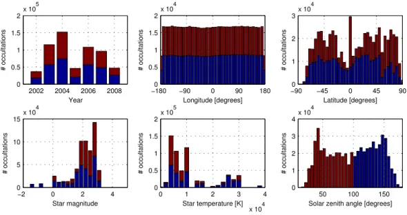
Fig. 1. Occultation statistics for the entire GOMOS data set spanning the period August 2002 - May 2008. Shown are histograms representing the number of GOMOS occultations as function of (from left to right, top to bottom) year, longitude, latitude, star magnitude, star temperature and solar zenith angle. Blue histograms refer to the fraction of occultations in dark limb, red ones to the fraction in bright limb.
ter sampling is obtained. The actual star spectrum is (in nor-mal mode) calculated from 7 CCD rows of the spectrometers, equivalent to a field of view of 0.01 degrees.
It is important to know that the uncertainty on the obtained profiles is largely determined by the magnitude and temper-ature of the observed star. But even bright stars (such as Sir-ius) are weak light sources in comparison with the Sun; pro-files obtained from stellar occultations have therefore larger uncertainties than the ones from solar occultations. This dis-advantage is however largely compensated for by the fact that stars are abundant in the sky: about 30 to 40 occulta-tions have been typically observed per orbit, although this number decreased to 20 or 30 occultations per orbit after an instrument malfunction in 2005. Hundreds of thousands of occultations have been observed by GOMOS since the start of the mission.
The occultation statistics for the period August 2002 - May 2008 (a total of about 600,000 events, the entire data set that was available to us at the time of writing) are represented by histograms in Fig. 1. Of course, the lower number of occultations for the years 2002 and 2008 are caused by an incomplete sampling of these years, while the smaller num-ber in 2005 resulted from the instrument failure mentioned earlier. Longitudinal sampling is clearly very homogeneous. Most occultations occur at midlatitudes, although plenty of polar measurements are available. Most stars have
moder-ate to weak brightness, and are rather cold. Also, about half of the occultations occur in the Sun-illuminated atmosphere (‘bright limb’, Solar Zenith Angle SZA < 100), the other half in ‘dark limb’ (SZA ≥ 100). More details about the solar il-lumination condition and its consequences are given below. 3 Retrieval method
3.1 Spectral behaviour
As already said above, the particle optical extinction trum is a priori unknown. Therefore, the actual optical spec-trum is treated as a product of the retrieval algorithm. It is far from clear how such a particle optical spectrum should be parameterized, but we can be guided by the fact that usual atmospheric particle size distributions are broad, covering a few orders of magnitude, and the resulting optical spectra are thus smooth. Hence they are often described with analytic, smooth functions, such as polynomials. For data version 6.0, the GOMOS Science team chose to implement a quadratic polynomial as a function of wavelength for the simple reason that it is versatile: large (constant spectrum), medium-sized (peak at mid-visible wavelengths) or small particle spectra (the Rayleigh limit: extinction β depends on wavelength λ as β ∼ λ−4) can within good approximation be captured
by such polynomials. Retrieval algorithms for other satellite
Fig. 1. Occultation statistics for the entire GOMOS data set spanning the period August 2002–May 2008. Shown are histograms representing
the number of GOMOS occultations as function of (from left to right, top to bottom) year, longitude, latitude, star magnitude, star temperature and solar zenith angle. Blue histograms refer to the fraction of occultations in dark limb, red ones to the fraction in bright limb.
(spectrometer B2). From measured signals, transmittances are calculated that in turn are used to derive altitude concen-tration profiles for O3, NO2, NO3, H2O and O2, and
temper-ature profiles. Furthermore, aerosol/cloud extinction profiles at different wavelengths are obtained.
The integration time to record a GOMOS full spectrum is 0.5 s. The actual vertical sampling is determined by this time, together with the vertical velocity of the tangent point (between 0.5 and 3.4 km/s, depending on the obliquity of the occultation) and refraction of the optical path at lower alti-tudes (which decreases the tangent point vertical velocity). A maximum vertical sampling resolution of 1.7 km can be expected, but during very oblique occultations a 200 meter sampling is obtained. The actual star spectrum is (in nor-mal mode) calculated from 7 CCD rows of the spectrometers, equivalent to a field of view of 0.01 degrees.
It is important to know that the uncertainty on the obtained profiles is largely determined by the magnitude and temper-ature of the observed star. But even bright stars (such as Sir-ius) are weak light sources in comparison with the Sun; pro-files obtained from stellar occultations have therefore larger uncertainties than the ones from solar occultations. This dis-advantage is however largely compensated for by the fact that stars are abundant in the sky: about 30 to 40 occulta-tions have been typically observed per orbit, although this number decreased to 20 or 30 occultations per orbit after an instrument malfunction in 2005. Hundreds of thousands of occultations have been observed by GOMOS since the start of the mission.
The occultation statistics for the period August 2002 - May 2008 (a total of about 600 000 events, the entire data set that was available to us at the time of writing) are represented by histograms in Fig. 1. Of course, the lower number of occultations for the years 2002 and 2008 are caused by an incomplete sampling of these years, while the smaller num-ber in 2005 resulted from the instrument failure mentioned earlier. Longitudinal sampling is clearly very homogeneous. Most occultations occur at midlatitudes, although plenty of polar measurements are available. Most stars have moder-ate to weak brightness, and are rather cold. Also, about half of the occultations occur in the Sun-illuminated atmosphere (“bright limb”, Solar Zenith Angle SZA<100), the other half in ‘dark limb’ (SZA≥100). More details about the solar illu-mination condition and its consequences are given below.
3 Retrieval method
3.1 Spectral behaviour
As already said above, the particle optical extinction trum is a priori unknown. Therefore, the actual optical spec-trum is treated as a product of the retrieval algorithm. It is far from clear how such a particle optical spectrum should be parameterized, but we can be guided by the fact that usual atmospheric particle size distributions are broad, covering a few orders of magnitude, and the resulting optical spectra are thus smooth. Hence they are often described with analytic, smooth functions, such as polynomials. For data version 6.0, the GOMOS Science team chose to implement a quadratic
8000 F. Vanhellemont et al.: GOMOS Aerosol/Cloud Extinction observations polynomial as a function of wavelength for the simple reason
that it is versatile: large (constant spectrum), medium-sized (peak at mid-visible wavelengths) or small particle spectra (the Rayleigh limit: extinction β depends on wavelength λ as
β∼λ−4) can within good approximation be captured by such polynomials. Retrieval algorithms for other satellite occul-tation instruments are often also equipped with this feature. Furthermore, Vanhellemont et al. (2006) showed with sim-ulated data (using a Mie code) that a quadratic polynomial is a good choice when one wants to obtain good aerosol re-trievals without introducing too many degrees of freedom in the retrieval problem.
3.2 Spectral/spatial inversion
The GOMOS retrieval algorithm has been described in de-tail in another paper of this special issue (Kyr¨ol¨a et al., 2010). Here it suffices to say that the retrieval consists of two parts: (1) the spectral inversion, where measured transmit-tance spectra at each tangent altitude separately are inverted to slant path integrated column densities (for gases) and op-tical thickness (for particles), and (2) the spatial or verop-tical inversion, where the retrievals of the first step are separately inverted to local concentration profiles (gases) and optical ex-tinction profiles (particles). This second step is performed in combination with a Tikhonov altitude smoothing (Twomey, 1985; Rodgers, 2000) in order to get partially rid of the per-turbations caused by residual scintillation in measurements taken during very inclined occultations (Sofieva et al., 2009). The amount of smoothing is determined by a predetermined target resolution for the profile. For particles, a profile reso-lution of 4 km was chosen since unsmoothed profiles showed strong oscillations; aerosol extinction spectra have the ten-dency to swallow a large portion of the residual scintillation perturbations. Nevertheless, fine-scale structures (e.g. thin clouds) are smeared out due to this feature. The choice of 4 km for target resolution was based on the experience that it gave agreeable results; the actual magnitude of the resid-ual scintillation perturbation on aerosol profiles is still not adequately determined, although it is known for the ozone retrievals (Sofieva et al., 2009).
It is in the spectral inversion model that the slant path par-ticle optical thickness is implemented as a quadratic polyno-mial:
τ (λ)=σref(r0+r11λ + r21λ2)
with 1λ=λ − λrefand λref=500 nm a reference wavelength.
For scaling purposes, a “cross section” σref=6×10⁻¹⁰cm2
was used. Notice that only the first parameter r0has a direct
physical meaning: σrefr0 equals the particle slant path
op-tical thickness at 500 nm. During the spatial inversion, this parameter receives Tikhonov-style altitude smoothing, while the other parameters remain unconstrained. Retrospectively, this turned out to be a poor methodology: while the obtained extinction profiles at 500 nm look quite good, the spectra at
other wavelengths (evaluated with the quadratic polynomial within the spectrometer A range 248-690 nm) are often very noisy.
Finally, it should be mentioned that during the spectral in-version, the optical extinction spectra from the neutral air (Rayleigh scattering) are removed instead of retrieved from the measurements, using external ECMWF (European Cen-tre for Medium-range Weather Forecasts) air density data, to avoid interferences with the residual scintillation and the spectrally similar aerosol contribution. Also, only spectrom-eter A measurements are currently used for the aerosol re-trieval.
3.3 The homogeneous layer assumption
Occultation measurements have a limited information con-tent. Hence the assumption of homogeneous atmospheric layers that is so often found in retrieval codes: the number of unknowns is drastically reduced, leading to a more stable inversion. For more or less uniformly mixed gases and par-ticles (such as stratospheric aerosols), the assumption should hold quite well. However, when local phenomena (such as clouds) are observed, the assumption is wrong: the phe-nomenon affects the light ray only locally. This should be taken into account whenever we analyse retrievals of PSCs and volcanic plumes, for example: the obtained extinction coefficients should be seen as slant path equivalent values.
3.4 Bright limb versus dark limb retrievals
When the optical light path traverses the Sun-illuminated atmosphere, parts of the atmosphere located in the field-of-view scatter additional light into the instrument, which means that the simple optical transmission model for the re-trieval is not correct anymore. This was anticipated: the addi-tionnal upper and lower CCD bands in GOMOS were imple-mented to correct for this background illumination (Bertaux et al., 2010; Kyr¨ol¨a et al., 2010). However, post-launch pro-cessing showed that the correction is not perfect. The sit-uation is particularly bad for the aerosol extinction profiles, since their smooth optical extinction spectrum strongly re-sembles the limb signal. The aerosol extinction retrievals typically show unrealistic features at very high stratospheric altitudes. At present, the best we can do is exclude the bright limb profiles from data analysis. Investigations showed that occultation events with a solar zenith angle of 100◦or larger deliver unperturbed, dark limb aerosol retrievals.
3.5 Retrieval results
In summary, the GOMOS particle extinction profiles have acceptable quality around 500 nm, but are oversmoothed. At other wavelenghts, the profile quality is poor, and we therefore exclude them from further study. Furthermore, it is best to exclude the aerosol profiles in bright limb
F. Vanhellemont et al.: GOMOS Aerosol/Cloud Extinction observations 8001
Vanhellemont et al.: GOMOS Aerosol/Cloud Extinction observations 5
0 2 4 x 10⁻³ 10 20 30 40 Extinction [km−1] Altitude [km]
Polar stratospheric cloud
0 2 4 x 10⁻³ 10 20 30 40 Extinction [km−1] Altitude [km]
Tropical subvisual cirrus
0 2 4 x 10⁻³ 10 20 30 40 Extinction [km−1] Altitude [km] Background aerosol 0 2 4 x 10⁻³ 10 20 30 40 Extinction [km−1] Altitude [km] Volcanic aerosol
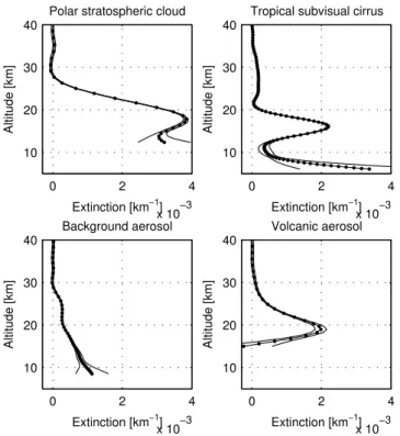
Fig. 2. Individual GOMOS particle extinction profiles with
as-sociated uncertainty: a Polar Stratospheric Cloud (2003/7/30,
72,57◦S, 2.18◦W), a tropical subvisual cirrus cloud (2002/10/7,
0.52◦S, 78.69◦E), background stratospheric aerosols (2003/9/12,
43.34◦S, 137.36◦W), volcanic stratospheric aerosols (2007/1/9,
4.52◦S, 27.15◦E). All plots have the same scale, in order to
facili-tate comparisons of magnitude.
introduce bias in the extinction profiles, as comparisons with other instruments show (see below).
Like all profiles derived from occultation measurements, GOMOS aerosol extinction profiles are increasingly more uncertain when we descend to lower altitudes, because the transmitted light intensity becomes weaker due to increas-ing atmospheric extinction by gases, aerosols and clouds. In principle, a cut-off altitude can be defined, below which no aerosol information is present anymore. This altitude de-pends on the wavelength considered, and the magnitude and temperature of the star, and therefore changes from one oc-cultation to the next. At 500 nm, an average limit of 10 km can be considered as a rough estimate below which the pro-files are not trustworthy anymore.
On Fig. 2, we present individual GOMOS extinction re-trievals at 500 nm for a number of particle types. It is impos-sible to distinguish these types using only one wavelength; the presented profiles were selected after analysis of the en-tire GOMOS data set and knowledge about geolocation and time of occurence of these particle phenomena (see further on in this paper).
It is clear that the profiles are oversmoothed. For instance,
tropical subvisual clouds are known to be horizontally ex-tended cloud layers that are quite thin, having a thickness smaller than 1 km (Jensen et al., 1996); the example on the figure clearly shows that the layer has been spread out by the smoothing constraint.
We should mention here that the obtained particle ex-tinction retrievals sometimes assume negative values, usu-ally at altitudes where the measured signals are low (below the above-mentioned cut-off altitude), or where the particle abundance is low (upper stratosphere and higher). This is a logical consequence of the fact that the last retrieval step (spatial inversion) is linear and that the retrievals are not con-strained to be positive. All further results that are discussed in this paper were obtained by processing of data that in-clude negative values; discarding these would lead to biased results.
Quantifying the aerosol extinction retrieval error is chal-lenging. A detailed description can be found in another pa-per of this GOMOS special issue (Tamminen et al., 2010). We repeat the most important ideas and findings here. The random error on a profile is determined by two contributions that we mentioned before: (1) the measurement noise which changes from one stellar source to another due to star mag-nitude and temperature differences, and (2) the uncorrected residual scintillation component. At the time of writing the GOMOS error estimation for the operational data products does not yet take the latter into account, so that retrieval er-rors are likely underestimated. The influence of star mag-nitude is clear: brighter stars deliver a better signal-to-noise ratio. Star temperature determines the main spectral emis-sion range: hot stars emit in the UV, colder ones in the vis-ible and near-infrared domain. The influence of star tem-perature on aerosol retrievals nevertheless remains limited; it is star magnitude that plays the crucial role (Tamminen et al., 2010). Sources of systematic error are of course (1) a possibly wrong aerosol spectral model, and (2) an imper-fect ECMWF air density profile, both of which have been estimated by Tamminen et al. (2010). Retrieval errors are of course calculated by standard error propagation through the retrieval chain. Aerosol extinction error estimates (for bright stars) of 30 % are obtained around an altitude of 10 km, 2-10 % from 15 to 25 km, and 10-50 % from 25 to 40 km.
As mentioned before, the amount of Tikhonov altitude smoothing is determined by a predefined target resolution of 4 km, at all altitudes, regardless of the star magnitude and temperature. Presentation of averaging kernels is therefore unnecessary; the profile resolution is chosen in advance.
4 Comparisons with other instruments
A detailed validation study for the GOMOS aerosol extinc-tion profiles has not been performed yet. Nevertheless, Van-hellemont et al. (2008) already performed comparisons with the results derived from the imagers of the Atmospheric
Fig. 2. Individual GOMOS particle extinction profiles with
associ-ated uncertainty: a Polar Stratospheric Cloud (30/7/2003, 72,57◦S,
2.18◦W), a tropical subvisual cirrus cloud (7/10/2002, 0.52◦S,
78.69◦E), background stratospheric aerosols (12/9/2003, 43.34◦S,
137.36◦W), volcanic stratospheric aerosols (9/1/2007, 4.52◦S,
27.15◦E). All plots have the same scale, in order to facilitate
com-parisons of magnitude.
(SZA<100): from the entire data set of 600 000 occulta-tions, about 301 000 remain to be exploited. Among these, some are still perturbed by residual scintillation. These per-turbations are visible in individual aerosol extinction profiles. When averaging large numbers of profiles (see e.g. the zonal plots below), the resulting mean profile becomes smooth. There is reason to assume that the scintillation perturbations do not introduce bias in the extinction profiles, as compar-isons with other instruments show (see below).
Like all profiles derived from occultation measurements, GOMOS aerosol extinction profiles are increasingly more uncertain when we descend to lower altitudes, because the transmitted light intensity becomes weaker due to increas-ing atmospheric extinction by gases, aerosols and clouds. In principle, a cut-off altitude can be defined, below which no aerosol information is present anymore. This altitude de-pends on the wavelength considered, and the magnitude and temperature of the star, and therefore changes from one oc-cultation to the next. At 500 nm, an average limit of 10 km can be considered as a rough estimate below which the pro-files are not trustworthy anymore.
On Fig. 2, we present individual GOMOS extinction re-trievals at 500 nm for a number of particle types. It is impos-sible to distinguish these types using only one wavelength; the presented profiles were selected after analysis of the en-tire GOMOS data set and knowledge about geolocation and time of occurence of these particle phenomena (see further on in this paper).
It is clear that the profiles are oversmoothed. For instance, tropical subvisual clouds are known to be horizontally ex-tended cloud layers that are quite thin, having a thickness smaller than 1 km (Jensen et al., 1996); the example on the figure clearly shows that the layer has been spread out by the smoothing constraint.
We should mention here that the obtained particle ex-tinction retrievals sometimes assume negative values, usu-ally at altitudes where the measured signals are low (below the above-mentioned cut-off altitude), or where the particle abundance is low (upper stratosphere and higher). This is a logical consequence of the fact that the last retrieval step (spatial inversion) is linear and that the retrievals are not con-strained to be positive. All further results that are discussed in this paper were obtained by processing of data that in-clude negative values; discarding these would lead to biased results.
Quantifying the aerosol extinction retrieval error is chal-lenging. A detailed description can be found in another pa-per of this GOMOS special issue (Tamminen et al., 2010). We repeat the most important ideas and findings here. The random error on a profile is determined by two contributions that we mentioned before: (1) the measurement noise which changes from one stellar source to another due to star mag-nitude and temperature differences, and (2) the uncorrected residual scintillation component. At the time of writing the GOMOS error estimation for the operational data products does not yet take the latter into account, so that retrieval er-rors are likely underestimated. The influence of star mag-nitude is clear: brighter stars deliver a better signal-to-noise ratio. Star temperature determines the main spectral emis-sion range: hot stars emit in the UV, colder ones in the vis-ible and near-infrared domain. The influence of star tem-perature on aerosol retrievals nevertheless remains limited; it is star magnitude that plays the crucial role (Tamminen et al., 2010). Sources of systematic error are of course (1) a possibly wrong aerosol spectral model, and (2) an imper-fect ECMWF air density profile, both of which have been estimated by Tamminen et al. (2010). Retrieval errors are of course calculated by standard error propagation through the retrieval chain. Aerosol extinction error estimates (for bright stars) of 30% are obtained around an altitude of 10 km, 2– 10% from 15 to 25 km, and 10-50% from 25 to 40 km.
As mentioned before, the amount of Tikhonov altitude smoothing is determined by a predefined target resolution of 4 km, at all altitudes, regardless of the star magnitude and temperature. Presentation of averaging kernels is therefore unnecessary; the profile resolution is chosen in advance.
8002 Vanhellemont et al.: GOMOS Aerosol/Cloud Extinction observationsF. Vanhellemont et al.: GOMOS Aerosol/Cloud Extinction observations7 −2000 −100 0 100 200 5 10 15 20 25 30 35 40 GOMOS/SAGE II Relative difference [%] Altitude [km] −2000 −100 0 100 200 5 10 15 20 25 30 35 40 GOMOS/SAGE III Relative difference [%] Altitude [km] −2000 −100 0 100 200 5 10 15 20 25 30 35 40 GOMOS/POAM III Relative difference [%] Altitude [km]
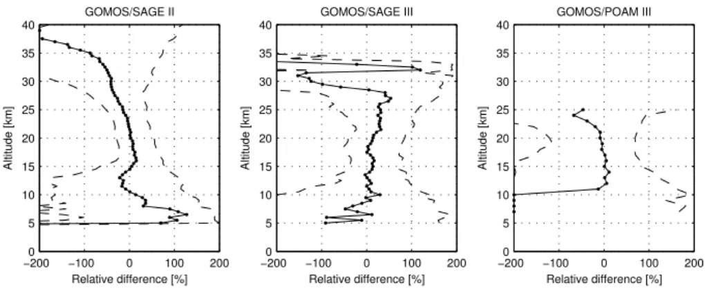
Fig. 3. Comparison of GOMOS aerosol extinction profiles with other satellite measurements: SAGE II at 525 nm (left panel), SAGE
III at 596 nm (middle panel) and POAM III at 603 nm (right panel). Shown are the statistics for the relative differences, calculated as
100× 2(pGOMOS− pSAT)/|pGOMOS+ pSAT|. The median of the set of relative differences is shown with full lines and dots. Dashed lines
indicate the spread, given by the 16th and 84th percentile.
−50 0 50 10 20 30 40 2002 Alt. [km] −50 0 50 10 20 30 40 2003 −50 0 50 10 20 30 40 2004 −50 0 50 10 20 30 40 2005 −50 0 50 10 20 30 40 2006 Lat. [deg.] Alt. [km] −50 0 50 10 20 30 40 2007 Lat. [deg.] −50 0 50 10 20 30 40 2008 Lat. [deg.] 0 0.2 0.4 0.6 0.8 1 x 10⁻³
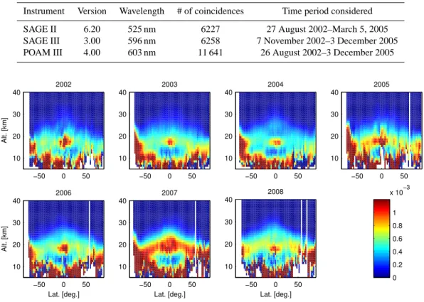
Fig. 4. Yearly zonal median values of (dark limb) aerosol extinction at 500 nm for the entire GOMOS mission. All features that are to be
expected are present: the stratospheric aerosol layer, PSCs in the Antarctic region, tropical subvisual cirrus clouds. Notice the enhanced stratospheric aerosol layer in 2007, resulting from the Soufri`ere Hills eruption in May 2006. Years that are sampled incompletely: 2002 (start of the data set: August 2002), 2005 (instrument failure) and 2008 (end of available data set).
Fig. 3. Comparison of GOMOS aerosol extinction profiles with other satellite measurements: SAGE II at 525 nm (left panel), SAGE
III at 596 nm (middle panel) and POAM III at 603 nm (right panel). Shown are the statistics for the relative differences, calculated as
100 × 2(pGOMOS−pSAT)/|pGOMOS+pSAT|. The median of the set of relative differences is shown with full lines and dots. Dashed lines
indicate the spread, given by the 16th and 84th percentile.
4 Comparisons with other instruments
A detailed validation study for the GOMOS aerosol extinc-tion profiles has not been performed yet. Nevertheless, Van-hellemont et al. (2008) already performed comparisons with the results derived from the imagers of the Atmospheric Chemistry Experiment ACE (Bernath et al., 2005). Here, we present first comparisons with aerosol extinction pro-files from the Stratospheric Aerosol and Gas Experiment II (SAGE II; see Chu et al. (1989)), its follow-up SAGE III (Thomason and Taha, 2003) and the Polar Ozone and Aerosol Measurement POAM III (Lucke et al., 1999). As al-ready stated, only dark limb measurements were considered. Furthermore we avoided PSCs by excluding occultations in-side the polar vortex: apart from the wrong assumption of homogeneous layers, two different instruments with two dif-ferent viewing geometries will deliver two difdif-ferent profiles for the same cloud. This is less of a problem for tropical subvisual cirrus since they typically have a very wide hor-izontal extent and are very thin. A coincidence window of +/−250 km and +/−6 h was used, allowing us to find a fairly large comparison data set, summarized in Table 1. The ge-ographic location of the obtained coincidences is mainly de-termined by the coverage of the used instruments (SAGE II, SAGE III and POAM III) since GOMOS has a near-global coverage with several occultation latitudes per orbit. Notice that we used a spectral channel of each instrument that is close to the GOMOS reference wavelength of 500 nm. Fur-thermore, GOMOS data were interpolated to these wave-lengths using the retrieved quadratic polynomial. We should also mention that no effort was made to match the vertical resolution between two instruments with averaging kernels; this will certainly be done in a full validation study in the future.
For the i-th coincidence, the difference between GOMOS (GOM) and the other instrument (SAT), relative to the mean of the two, was evaluated as follows:
1i=100 × 2
(pGOM,i−pSAT,i)
|pGOM,i+pSAT,i|
As statistical estimators for the entire data set, we prefered to use the median (50th percentile) since it is more robust with respect to outliers than the numerical mean. The vari-ance of the data set was calculated with the 16th and 84th percentile. The obtained statistical estimates are shown in Fig. 3. As can be seen, the comparisons are quite good at upper tropospheric/lower stratospheric altitudes. Differences with SAGE II are within 20% from 10 to 25 km, a conclusion that can also be drawn for the SAGE III comparisons. The median differences with POAM III are even smaller, within 10% from 11 to 22 km. Notice however that the variance is much larger than for the SAGE II/III comparisons.
5 Results
5.1 Yearly zonal statistics
A coarse idea about the presence of aerosols and clouds in the upper troposphere/lower stratosphere can be gained by considering zonal yearly statistics. Ranging from 90◦S to 90◦N, 72 latitude bins with a width of 2.5 degrees were de-fined. Aerosol extinction profiles were linearly interpolated on a common altitude grid ranging from 1 to 50 km with a spacing of 1 km. Yearly statistics were subsequently calcu-lated on all data within one bin. Once again: we used per-centiles as statistical estimators since extinction values are not necessarily normally distributed and because the median (50th percentile) is rather insensitive to outliers. We should
F. Vanhellemont et al.: GOMOS Aerosol/Cloud Extinction observations 8003
Table 1. GOMOS aerosol extinction retrievals: comparison data set; coincidence window: (500 km, 1/2 day)
Instrument Version Wavelength # of coincidences Time period considered
SAGE II 6.20 525 nm 6227 27 August 2002–March 5, 2005
SAGE III 3.00 596 nm 6258 7 November 2002–3 December 2005
POAM III 4.00 603 nm 11 641 26 August 2002–3 December 2005
Vanhellemont et al.: GOMOS Aerosol/Cloud Extinction observations 7
−2000 −100 0 100 200 5 10 15 20 25 30 35 40 GOMOS/SAGE II Relative difference [%] Altitude [km] −2000 −100 0 100 200 5 10 15 20 25 30 35 40 GOMOS/SAGE III Relative difference [%] Altitude [km] −2000 −100 0 100 200 5 10 15 20 25 30 35 40 GOMOS/POAM III Relative difference [%] Altitude [km]
Fig. 3. Comparison of GOMOS aerosol extinction profiles with other satellite measurements: SAGE II at 525 nm (left panel), SAGE III at 596 nm (middle panel) and POAM III at 603 nm (right panel). Shown are the statistics for the relative differences, calculated as 100× 2(pGOMOS− pSAT)/|pGOMOS+ pSAT|. The median of the set of relative differences is shown with full lines and dots. Dashed lines indicate the spread, given by the 16th and 84th percentile.
−50 0 50 10 20 30 40 2002 Alt. [km] −50 0 50 10 20 30 40 2003 −50 0 50 10 20 30 40 2004 −50 0 50 10 20 30 40 2005 −50 0 50 10 20 30 40 2006 Lat. [deg.] Alt. [km] −50 0 50 10 20 30 40 2007 Lat. [deg.] −50 0 50 10 20 30 40 2008 Lat. [deg.] 0 0.2 0.4 0.6 0.8 1 x 10⁻³
Fig. 4. Yearly zonal median values of (dark limb) aerosol extinction at 500 nm for the entire GOMOS mission. All features that are to be expected are present: the stratospheric aerosol layer, PSCs in the Antarctic region, tropical subvisual cirrus clouds. Notice the enhanced stratospheric aerosol layer in 2007, resulting from the Soufri`ere Hills eruption in May 2006. Years that are sampled incompletely: 2002 (start of the data set: August 2002), 2005 (instrument failure) and 2008 (end of available data set).
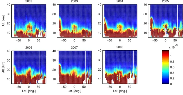
Fig. 4. Yearly zonal median values of (dark limb) aerosol extinction at 500 nm for the entire GOMOS mission. All features that are to be
expected are present: the stratospheric aerosol layer, PSCs in the Antarctic region, tropical subvisual cirrus clouds. Notice the enhanced stratospheric aerosol layer in 2007, resulting from the Soufri`ere Hills eruption in May 2006. Years that are sampled incompletely: 2002 (start of the data set: August 2002), 2005 (instrument failure) and 2008 (end of available data set).
also mention that yearly zonal statistics are seasonally bi-ased when we use only dark limb measurements, since Arc-tic/Antarctic summer is not sampled. The median particle extinction at 500 nm is shown in Fig. 4 for every GOMOS mission year. A few phenomena are readily observed: (1) the umbrella-shaped stratospheric aerosol layer that is high-est at the equator, lowhigh-est at the poles, (2) higher extinction values in the Antarctic (and to a lesser extent Arctic) strato-sphere that are caused by PSCs, and (3) higher extinction values in a localized tropical zone at an altitude of about 16– 17 km due to subvisual cirrus clouds. The picture is almost systematic for every year, but there are some significant dif-ferences however. First notice that Antarctic PSCs are less pronounced for the years 2002 and 2008 because the Antarc-tic PSC season is not well sampled in those years: the data set starts end of August 2002 and ends in May 2008. More important, stratospheric aerosol extinction levels are much higher in 2007 and remain elevated even in 2008, suggesting the formation of new aerosols following stratospheric injec-tion of SO2 by a volcanic eruption. This is the case; the
Soufri`ere Hills eruption (see below) in May 2006 is most
likely the source. Furthermore, 2005 also seems to exhibit elevated aerosol levels, although the picture is noisier due to the incomplete sampling of the year (instrument failure).
Equally interesting is the yearly zonal variability of the 500 nm aerosol extinction values, calculated as half the dif-ference between the 84th and 16th percentile. The variabil-ity is of course determined by the S/N-ratio of the mea-surements and (more importantly) by natural aerosol/cloud variability, caused by the appearing, disappearing and at-mospheric transport of particles. This is clearly visible on Fig. 5. Typical “on/off-events” such as clouds (tropical cir-rus, PSCs) exhibit large variability, while slowly changing features (such as the stratospheric aerosol layer) vary little within one year. Notice once again that the Antarctic PSC variability during 2002 and 2008 is weak since these years have not been completely sampled. At lower, tropospheric altitudes, we see large variability due to a combination of larger profile uncertainty (measured signals are weaker) and tropospheric clouds.
8004 F. Vanhellemont et al.: GOMOS Aerosol/Cloud Extinction observations
8 Vanhellemont et al.: GOMOS Aerosol/Cloud Extinction observations
Table 1. GOMOS aerosol extinction retrievals: comparison data set; coincidence window: (500 km, 1/2 day) Instrument Version Wavelength # of coincidences Time period considered
SAGE II 6.20 525 nm 6227 August 27, 2002 - March 5, 2005
SAGE III 3.00 596 nm 6258 November 7, 2002 - December 3, 2005
POAM III 4.00 603 nm 11641 August 26, 2002 - December 3, 2005
−50 0 50 10 20 30 40 2002 Alt. [km] −50 0 50 10 20 30 40 2003 −50 0 50 10 20 30 40 2004 −50 0 50 10 20 30 40 2005 −50 0 50 10 20 30 40 2006 Alt. [km] Lat. [deg.] −50 0 50 10 20 30 40 2007 Lat. [deg.] −50 0 50 10 20 30 40 2008 Lat. [deg.] 0 0.2 0.4 0.6 0.8 1 x 10⁻³
Fig. 5. Yearly zonal variability of (dark limb) aerosol extinction at 500 nm for the entire GOMOS mission. Variability is calculated as half the difference of the 84th and 16th percentile, and is determined by measurement error and (more importantly) by natural aerosol/cloud variability. ’On/off’ events such as clouds (tropical cirrus, Antarctic PSCs) of course exhibit large variability, while slowly changing features (backgrounds aerosol layer) vary little. Years that are sampled incompletely: 2002 (start of the data set: august 2002), 2005 (instrument failure) and 2008 (end of available data set).
2006, in a tropical latitude band from 6◦N to 26◦N. Three distinct periods can be seen. First, we observe low back-ground aerosol levels until the end of 2004. Second, from early 2005 to the beginning of June 2006, large data gaps are present due to instrument failure. Nevertheless, the data seem to suggest a declining tail following a volcanic erup-tion, especially if we take the small set of data points at early 2005 into account. And third, in early July 2006 we observe a sudden increase by about a factor of 3 in extinction levels. The same conclusions are drawn when inspecting the evolu-tion in latitude and time on Fig. 7. It is clear that at least two volcanic events in the tropics should be considered.
The elevated values in 2005 are most likely caused by stratospheric sulfate aerosols, formed out of the SO2cloud injected in the stratosphere by the eruptions of the Manam volcano (Papua New Guinea, 4.080◦S, 145.037◦E) on
Jan-uary 27 and 28 (Kamei et al., 2006). Manam is one of the most active volcanoes in the region; the above men-tioned eruptions followed ongoing volcanic activity that started already in October 2004. An image taken by the infrared Aqua/MODIS (Moderate Resolution Imaging Spec-troradiometer) indicates that the ash clouds of the first erup-tion on Jan. 27 reached to over 20 km altitude, well into the stratosphere. The ash clouds of the second eruption on Jan. 28 ascended to 18 km altitude (Smithsonian Institution, 2005). Several days later, stratospheric aerosol layers were detected twice between about 18 to 20 km altitude (layer thickness ranging from 0.2 to 1.4 km) by a shipboard lidar us-ing a Nd:YAG laser operated at 1064 nm and 532 nm (Kamei et al., 2006). The layers were detected in the Western Pacific around 0 - 2◦N, 156◦E (Feb. 3-4 2005) and 7 - 9◦N, 156◦E (Feb. 9 - 10). Inspecting Fig. 7, we see that the amount of
Fig. 5. Yearly zonal variability of (dark limb) aerosol extinction at 500 nm for the entire GOMOS mission. Variability is calculated as
half the difference of the 84th and 16th percentile, and is determined by measurement error and (more importantly) by natural aerosol/cloud variability. “On/off” events such as clouds (tropical cirrus, Antarctic PSCs) of course exhibit large variability, while slowly changing features (backgrounds aerosol layer) vary little. Years that are sampled incompletely: 2002 (start of the data set: august 2002), 2005 (instrument
failure) and 2008 (end of available data set).Vanhellemont et al.: GOMOS Aerosol/Cloud Extinction observations 9
Feb04 Jun04 Sep04 Dec04 Mar05 Jul05 Oct05 Jan06 May06 Aug06 Nov06
−1 −0.5 0 0.5 1 1.5 2 2.5 3x 10 −3 Aerosol. Ext. [1/km] Date
2004 to 2006 − Aerosol ext. 500 nm, alt. = 20 km, lat. = 6°N − 26°N
Fig. 6. A 2004-2006 GOMOS aerosol extinction time series at an altitude of 20 km. All data within a latitude band from 6◦N - 26◦N are
shown. Clearly visible are the background aerosol condition in 2004, the possible declining tail of the post-eruptive aerosols resulting from the Manam volcano (Papua New Guinea, Jan. 27-28, 2005; first vertical line), and the enhanced aerosol levels following the eruption of Soufri`ere Hills (Montserrat, May 20, 2006, second vertical line).
injected sulfur was large enough to leave a significant aerosol trace in the GOMOS data during the largest part of 2005.
The source for the elevated aerosol levels in the second half of 2006 and 2007 has been identified as the eruption of the Soufri`ere Hills volcano (16.72◦N, 62.18◦W, Montser-rat, West Indies), on May 20, 2006. Immediately following the collapse of the eastern volcano flank, an eruption column of ash and gases rose to at least 17 km. Prata et al. (2007) used a combination of satellite instruments (Aqua/AIRS, MSG/SEVIRI, MLS, OMI and CALIPSO/CALIOP) to re-construct the event and its immediate aftermath. They found that an estimated 0.1 Tg(S) was injected in the stratosphere in the form of SO2, after which the gas cloud traveled west-ward at an altitude of about 20 km. Carn et al. (2007) on the other hand used OMI data to obtain an estimated 0.22 Tg of SO2. They also reported CALIPSO/CALIOP li-dar backscatter measurements of the associated stratospheric aerosol layer as early as June 7, 2006, at an altitude of 20 km. The layer remained visible in the CALIOP data until July 6. However, as Thomason et al. (2007) remarked, in gen-eral the stratospheric aerosol layer remains quite invisible in CALIOP backscatter measurements, while occulation
instru-path lengths. Nevertheless, very recently Vernier et al. (2009) showed how CALIPSO/CALIOP backscatter data improved strongly after the introduction of a new cloud mask and a new calibration, and how an improved stratospheric aerosol picture emerged after sufficient data averaging. In any case, the fact that GOMOS identifies stratospheric sulfate aerosols well after the eruption date is illustrated in Fig. 8, which shows the appearing and poleward transport of the sulfuric acid particles.
Figs. 7 and 8 also indicate that it took roughly one year for the Soufri`ere Hills aerosol cloud to cover the entire globe. Elevated extinction levels remained present until at least the end of 2007. In the months following the Soufri`ere Hills eruption, a few other eruptions possibly impacted the strato-spheric aerosol layer. Hofmann et al. (2009) briefly men-tioned the July 14, 2006 Tungurahua eruption (Ecuador, 1,467◦S, 78,442◦W), less than a month after the Soufri`ere Hills eruption. And Thomason et al. (2007) showed CALIOP observations of the volcanic plume resulting from the Octo-ber 7, 2006 Tavurvur eruption (Rabaul, Papua New Guinea, 4.271◦S, 152.203◦E). Both are equatorial volcanoes that pos-sible injected sulfur into the stratosphere, hereby
enhanc-Fig. 6. A 2004-2006 GOMOS aerosol extinction time series at an altitude of 20 km. All data within a latitude band from 6–26◦N are shown. Clearly visible are the background aerosol condition in 2004, the possible declining tail of the post-eruptive aerosols resulting from the Manam volcano (Papua New Guinea, Jan. 27-28, 2005; first vertical line), and the enhanced aerosol levels following the eruption of Soufri`ere Hills (Montserrat, 20 May 2006, second vertical line).
5.2 Volcanic stratospheric aerosols
The observed elevated extinction levels in 2005 and 2007 re-quire a more detailed investigation. On Fig. 6, we present aerosol extinction values at an altitude of 20 km (which lies above the subvisual cirrus altitudes) for the period 2004– 2006, in a tropical latitude band from 6◦N to 26◦N. Three
distinct periods can be seen. First, we observe low back-ground aerosol levels until the end of 2004. Second, from early 2005 to the beginning of June 2006, large data gaps are present due to instrument failure. Nevertheless, the data seem to suggest a declining tail following a volcanic erup-tion, especially if we take the small set of data points at early 2005 into account. And third, in early July 2006 we observe
F. Vanhellemont et al.: GOMOS Aerosol/Cloud Extinction observations10 Vanhellemont et al.: GOMOS Aerosol/Cloud Extinction observations 8005
Jan05 Jan06 Jan07 Jan08 −90 −45 0 45 90 Lat. [deg.]
Aerosol extinction (500 nm) at 18 km altitude
0 0.5 1 1.5 2 x 10⁻³
Jan05 Jan06 Jan07 Jan08 −90 −45 0 45 90 Lat. [deg.]
Aerosol extinction (500 nm) at 20 km altitude
0 0.5 1 1.5 2 x 10⁻³
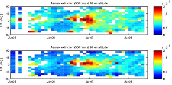
Fig. 7. Checkerboard plots showing the median of binned 500 nm aerosol extinction data as function of latitude and time, at an altitude of 18 km (upper panel) and 20 km (lower panel). Notice the elevated values after early 2005, and after the end of May 2006. The global spreading is clearly visible in the latter case.
et al. (2009). From GOMOS data it is at present unclear wether or not the existing volcanic aerosol layer was replen-ished with new sulfate aerosols originating from these erup-tions.
5.3 Polar Stratospheric Clouds
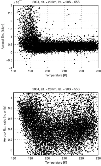
GOMOS detects PSCs quite well. Strongly enhanced opti-cal extinction is measured every year in the Antarctic PSC season (roughly from the end of May to October), with val-ues typically 3 or 4 times larger than in normal background conditions. These kind of criteria (latitude, time of year, ex-tinction values above a certain treshold) allow us to identify the presence of a PSC. It is however temperature that is the main driver for the formation of PSCs, as can be seen on the top panel of Fig. 9. Shown are all GOMOS aerosol ex-tinction measurements at 500 nm taken in 2004 at an alti-tude of 20 km for the latialti-tude band from 90◦S to 55◦S. Tem-perature data were obtained from the GOMOS product files and consist of ECMWF analysis profiles. The selected data set represents a mixture of measurements inside and outside the Antarctic vortex (PSCs and stratospheric aerosols), but plotted against temperature the differentiation is very clear: clouds are formed below about 195 K, the known forma-tion temperature of NAT and STS PSCs. It is however less clear from the data whether or not Type II PSCs form at even lower temperatures. Ideally, differentiation of different types
of PSC with UV/Vis/NIR data should be done by inspecting particle size distributions, or the shape of the associated opti-cal spectrum. Methods have already been devised in the past for the SAGE and POAM instruments to make a distinction between Type Ia and Ib particles, based on the assumption that the latter are smaller than the former, with a different extinction spectrum as a consequence (Strawa et al., 2002; Poole et al., 2003). The second panel of Fig. 9 shows the ratio of 600 nm to 400 nm GOMOS optical extinction. The-oretically, very small particles (β(λ) ∼ λ−4) should lead to a value of 0.2, while large particles (β(λ) = constant) should have a value of 1. The data are extremely noisy due to the already mentioned problem with the aerosol spectral law im-plementation. Nevertheless, the data cloud is more or less situated between the theoretical limits, and larger particles are observed below 195 K, as expected. The data show also that it is currently impossible to differentiate between differ-ent PSC types.
The presented PSC results do not add significantly new in-formation to the current knowledge on PSC in-formation; for this, much more detailed analysis is needed (taking into ac-count all thermodynamic parameters and air parcel dynam-ics). But the GOMOS measurements clearly contain ele-ments (temperature dependence of extinction and particle sizes) that are crucial in such a detailed study.
Fig. 7. Checkerboard plots showing the median of binned 500 nm aerosol extinction data as function of latitude and time, at an altitude
of 18 km (upper panel) and 20 km (lower panel). Notice the elevated values after early 2005, and after the end of May 2006. The global spreading is clearly visible in the latter case.
a sudden increase by about a factor of 3 in extinction levels. The same conclusions are drawn when inspecting the evolu-tion in latitude and time on Fig. 7. It is clear that at least two volcanic events in the tropics should be considered.
The elevated values in 2005 are most likely caused by stratospheric sulfate aerosols, formed out of the SO2 cloud
injected in the stratosphere by the eruptions of the Manam volcano (Papua New Guinea, 4.080◦S, 145.037◦E) on Jan-uary 27 and 28 (Kamei et al., 2006). Manam is one of the most active volcanoes in the region; the above men-tioned eruptions followed ongoing volcanic activity that started already in October 2004. An image taken by the infrared Aqua/MODIS (Moderate Resolution Imaging Spec-troradiometer) indicates that the ash clouds of the first erup-tion on 27 January reached to over 20 km altitude, well into the stratosphere. The ash clouds of the second eruption on Jan. 28 ascended to 18 km altitude (Smithsonian Institu-tion, 2005). Several days later, stratospheric aerosol lay-ers were detected twice between about 18 to 20 km altitude (layer thickness ranging from 0.2 to 1.4 km) by a shipboard lidar using a Nd:YAG laser operated at 1064 nm and 532 nm (Kamei et al., 2006). The layers were detected in the Western Pacific around 0–2◦N, 156◦E (3–4 February 2005) and 7– 9◦N, 156◦E (9–10 February). Inspecting Fig. 7, we see that the amount of injected sulfur was large enough to leave a sig-nificant aerosol trace in the GOMOS data during the largest part of 2005.
The source for the elevated aerosol levels in the second half of 2006 and 2007 has been identified as the eruption of the Soufri`ere Hills volcano (16.72◦N, 62.18◦W, Montser-rat, West Indies), on 20 May 2006. Immediately following the collapse of the eastern volcano flank, an eruption column
of ash and gases rose to at least 17 km. Prata et al. (2007) used a combination of satellite instruments (Aqua/AIRS, MSG/SEVIRI, MLS, OMI and CALIPSO/CALIOP) to re-construct the event and its immediate aftermath. They found that an estimated 0.1 Tg(S) was injected in the stratosphere in the form of SO2, after which the gas cloud traveled
west-ward at an altitude of about 20 km. Carn et al. (2007) on the other hand used OMI data to obtain an estimated 0.22 Tg of SO2. They also reported CALIPSO/CALIOP
li-dar backscatter measurements of the associated stratospheric aerosol layer as early as 7 June 2006, at an altitude of 20 km. The layer remained visible in the CALIOP data until 6 July. However, as Thomason et al. (2007) remarked, in gen-eral the stratospheric aerosol layer remains quite invisible in CALIOP backscatter measurements, while occulation instru-ments such as SAGE II have no problem with the detection. No doubt this is caused by the preferential forward scattering of light by small particles, in combination with longer optical path lengths. Nevertheless, very recently Vernier et al. (2009) showed how CALIPSO/CALIOP backscatter data improved strongly after the introduction of a new cloud mask and a new calibration, and how an improved stratospheric aerosol picture emerged after sufficient data averaging. In any case, the fact that GOMOS identifies stratospheric sulfate aerosols well after the eruption date is illustrated in Fig. 8, which shows the appearing and poleward transport of the sulfuric acid particles.
Figures 7 and 8 also indicate that it took roughly one year for the Soufri`ere Hills aerosol cloud to cover the entire globe. Elevated extinction levels remained present until at least the end of 2007. In the months following the Soufri`ere Hills eruption, a few other eruptions possibly impacted the
8006 F. Vanhellemont et al.: GOMOS Aerosol/Cloud Extinction observations
Vanhellemont et al.: GOMOS Aerosol/Cloud Extinction observations 11
−50 0 50 10 20 30 Alt. [km] May 2006 −50 0 50 10 20 30 June 2006 −50 0 50 10 20 30 July 2006 −50 0 50 10 20 30 Aug. 2006 −50 0 50 10 20 30 Alt. [km] Sep. 2006 −50 0 50 10 20 30 Oct. 2006 −50 0 50 10 20 30 Lat. Nov. 2006 −50 0 50 10 20 30 Lat. Dec. 2006 −50 0 50 10 20 30 Lat. Alt. [km] Jan. 2007 −50 0 50 10 20 30 Lat. Feb. 2007 −50 0 50 10 20 30 Lat. Mar. 2007 −50 0 50 10 15 20 25 30 Lat. Apr. 2007 0 0.2 0.4 0.6 0.8 1 1.2 1.4 1.6 1.8 2 x 10⁻³
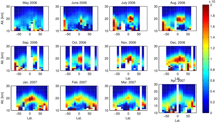
Fig. 8. Evolution of the volcanic stratospheric aerosols resulting from the Soufri`ere Hills eruption on May 20, 2006. Shown are monthly
zonal median aerosol extinction coefficients at 500 nm. Starting from the eruption site (Montserrat, 16.72◦N, 62.18◦W), the plume disperses
poleward and encircles the entire earth within a year. 6 Conclusions
The current GOMOS operational aerosol/cloud product con-sists of optical extinction profiles at 500 nm and additional spectral coefficients to evaluate the extinction at other wave-lengths as well. The quality of the product is not optimal yet, due to a problematic spectral law implementation, combined with an altitude smoothing that is too strong. Furthermore, profiles derived from bright limb measurements are currently not usable. Nevertheless, if we restrict ourselves to the use of 500 nm extinction profiles retrieved from dark limb measure-ments, then the quality can be considered as good, although fine structure (thin cirrus clouds, cloud inhomogeneities etc.) has been smoothed. For the first time, a comparison with SAGE II, SAGE III and POAM III was presented, showing good agreement within 20 % in the upper troposphere/lower stratosphere, from 10 km to about 25 km.
All the atmospheric particle types that are expected to be observed by a satellite occultation instrument have been detected by GOMOS: the background stratospheric sulfate aerosol layer (or Junge layer) with its typical umbrella-shaped form, sulfate aerosols from volcanic origin, tropical subvisual cirrus clouds just below the tropopause at an al-titude of about 16-17 km, and PSCs in the polar regions.
The cloud-type events (PSCs and cirrus) have a strong yearly variability, while the Junge layer remains remarkably con-stant within one year.
The last major volcanic SO2injection into the stratosphere
dates already from almost 18 years ago (Mount Pinatubo, 1991), with the consequence that current aerosol levels are extremely low. So low that the effect of ‘moderate’ vol-canic eruptions becomes visible in the GOMOS aerosol record. One might wonder if the so-called background is not only maintained by the typically mentioned sources (OCS, recently even anthropogenic sulfate from coal burning in China), but as well by these moderate volcanic eruptions, that are much weaker than the catastrophic events (Mt. Pinatubo, Mt. St. Helens, El Chich´on), but much more frequent. Here, for the first time, the aerosol enhancements resulting from the eruptions of Manam (Papua New Guinea) and Soufri`ere Hills (Montserrat, West Indies) have been identified in the GOMOS data. In the latter case, GOMOS was clearly able to track the global dispersion of the aerosols. In the aftermath of the eruption, two other possible intrusions should in prin-ciple be visible: Tungurahua (Ecuador) and Tavurvur (Papua New Guinea). We hope to identify them in future aerosol profile improvements.
The dynamics of PSCs have been studied previously with
Fig. 8. Evolution of the volcanic stratospheric aerosols resulting from the Soufri`ere Hills eruption on 20 May 2006. Shown are monthly
zonal median aerosol extinction coefficients at 500 nm. Starting from the eruption site (Montserrat, 16.72◦N, 62.18◦W), the plume disperses
poleward and encircles the entire earth within a year.
stratospheric aerosol layer. Hofmann et al. (2009) briefly mentioned the 14 July 2006 Tungurahua eruption (Ecuador, 1,467◦S, 78,442◦W), less than a month after the Soufri`ere Hills eruption. And Thomason et al. (2007) showed CALIOP observations of the volcanic plume resulting from the Octo-ber 7, 2006 Tavurvur eruption (Rabaul, Papua New Guinea, 4.271◦S, 152.203◦E). Both are equatorial volcanoes that possible injected sulfur into the stratosphere, hereby enhanc-ing the already existenhanc-ing Soufri`ere Hills perturbation. The Tavurvur case was recently demonstrated in a convincing way using the improved CALIPSO/CALIOP data by Vernier et al. (2009). From GOMOS data it is at present unclear wether or not the existing volcanic aerosol layer was replen-ished with new sulfate aerosols originating from these erup-tions.
5.3 Polar Stratospheric Clouds
GOMOS detects PSCs quite well. Strongly enhanced opti-cal extinction is measured every year in the Antarctic PSC season (roughly from the end of May to October), with val-ues typically 3 or 4 times larger than in normal background conditions. These kind of criteria (latitude, time of year, ex-tinction values above a certain treshold) allow us to identify
the presence of a PSC. It is however temperature that is the main driver for the formation of PSCs, as can be seen on the top panel of Fig. 9. Shown are all GOMOS aerosol ex-tinction measurements at 500 nm taken in 2004 at an alti-tude of 20 km for the latialti-tude band from 90◦S to 55◦S. Tem-perature data were obtained from the GOMOS product files and consist of ECMWF analysis profiles. The selected data set represents a mixture of measurements inside and outside the Antarctic vortex (PSCs and stratospheric aerosols), but plotted against temperature the differentiation is very clear: clouds are formed below about 195 K, the known formation temperature of NAT and STS PSCs. It is however less clear from the data whether or not Type II PSCs form at even lower temperatures. Ideally, differentiation of different types of PSC with UV/Vis/NIR data should be done by inspecting particle size distributions, or the shape of the associated opti-cal spectrum. Methods have already been devised in the past for the SAGE and POAM instruments to make a distinction between Type Ia and Ib particles, based on the assumption that the latter are smaller than the former, with a different extinction spectrum as a consequence (Strawa et al., 2002; Poole et al., 2003). The second panel of Fig. 9 shows the ratio of 600 nm to 400 nm GOMOS optical extinction. The-oretically, very small particles (β(λ)∼λ−4) should lead to a