HAL Id: inserm-00752896
https://www.hal.inserm.fr/inserm-00752896
Submitted on 16 Nov 2012
HAL is a multi-disciplinary open access archive for the deposit and dissemination of sci-entific research documents, whether they are pub-lished or not. The documents may come from
L’archive ouverte pluridisciplinaire HAL, est destinée au dépôt et à la diffusion de documents scientifiques de niveau recherche, publiés ou non, émanant des établissements d’enseignement et de
application to robust MRI brain scan segmentation
Florence Forbes, Scherrer Benoît, Dojat Michel
To cite this version:
Florence Forbes, Scherrer Benoît, Dojat Michel. Bayesian Markov model for cooperative cluster-ing: application to robust MRI brain scan segmentation. Journal de la Societe Française de Statis-tique, Societe Française de Statistique et Societe Mathematique de France, 2011, 152 (3), pp.116-141. �inserm-00752896�
Submission
Bayesian Markov model for cooperative clustering:
application to robust MRI brain scan segmentation
Titre: Approche bayesienne et markovienne pour des classifications couplées coopératives : application à la segmentation d’IRM du cerveau
Florence Forbes1, Benoit Scherrer2and Michel Dojat2
Abstract: Clustering is a fundamental data analysis step that consists of producing a partition of the observations to account for the groups existing in the observed data. In this paper, we introduce an additional cooperative aspect. We address cases in which the goal is to produce not a single partition but two or more possibly related partitions using cooperation between them. Cooperation is expressed by assuming the existence of two sets of labels (group assignments) which are not independent. We also model additional interactions by considering dependencies between labels within each label set. We propose then a cooperative setting formulated in terms of conditional Markov Random Field models for which we provide alternating and cooperative estimation procedures based on variants of the Expectation Maximization (EM) algorithm for inference. We illustrate the advantages of our approach by showing its ability to deal successfully with the complex task of segmenting simultaneously and cooperatively tissues and structures from MRI brain scans.
Résumé : La classification est une étape clef de l’analyse de données qui consiste à produire une partition des données qui traduise l’existence de groupes dans celles-ci. Dans cet article, nous introduisons la notion de classifications coopératives. Nous considérons le cas où l’objectif est de produire deux (ou plus) partitions des données de manière non indépendante mais en prenant en compte les informations que l’une des partitions apporte sur l’autre et réciproquement. Pour ce faire, nous considérons deux (ou plus) jeux d’étiquettes non indépendants. Des interactions supplémentaires entre étiquettes au sein d’un même jeu sont également modélisées pour prendre en compte par exemple des dépendances spatiales. Ce cadre coopératif est formulé à l’aide de modèles de champs de Markov conditionnels dont les paramètres sont estimés par une variante de l’algorithme EM. Nous illustrons les performances de notre approche sur un problème réel difficile de segmentation simultanée des tissus et des structures du cerveau à partir d’images de résonnance magnétique artefactées.
Keywords: Model-based clustering, Markov random fields, Bayesian analysis, EM algorithm, Generalized alternating maximization, Human Brain
Mots-clés : Classification à base de modèles, Champs de Markov, Analyse bayesienne, Algorithme EM, Maximization alternée généralisée, Cerveau humain
AMS 2000 subject classifications: 62F15, 62P10
1. Introduction
Clustering or segmentation of data is a fundamental data analysis step that has received increasing interest in recent years due to the emergence of several new areas of application. Attention has been focused on clustering various data type, regular vector data, curve data or more heterogeneous data
1 INRIA Grenoble Rhône-Alpes, Grenoble University, Laboratoire Jean Kuntzman, France. E-mail:[email protected]
2 INSERM, Grenoble Insitute of Neuroscience, Grenoble University, France.
[8]. In these cases, the goal is to produce a single partition of the observations (eg. via a labelling of each data point) that accounts for the groups existing in the observed data. The issue we consider in this paper is that of producing more than one partition using the same data. Examples of applications in which this is relevant include tissue and structure segmentation in Magnetic Resonance (MR) brain scan analysis [26], simultaneous estimation of motion discontinuities and optical flow in motion analysis [17], consistent depth estimation and boundary [22] or depth discontinuity [28] detection, etc. To address this goal, we consider a probabilistic missing data framework and assume the existence of two (or more) sets of missing variables. These sets represent two (or more) sets of labels which are related in the sense that information on one of them can help in finding the other. It follows that there is a clear gain in considering the two sets of labels in a single cooperative modelling. Beyond the need for modelling cooperation, in many applications, data points are not independent and require models that account for dependencies. For this purpose, we use Markov random field (MRF) models to further specify our missing data framework. In most non trivial cases, this results in complex systems that include processes interacting on a wide variety of scales. One approach to complicated processes in the presence of data is hierarchical modelling. Hierarchical modelling is based on a decomposition of the problem that corresponds to a factorization of the joint distribution
p(y,z,θ) = p(y|z,θ)p(z|θ)p(θ), (1)
whereY, Z, Θ are random variables denoting respectively the data, the labels and the parameters. We use capital letters to indicate random variables while their realizations are denoted with small letters.
In our cooperative setting, we focus more particularly on situations where the p(z|θ) part is made of different sub-processes which are linked and provide complementary information. We propose an approach different from the standard hierarchical modelling. Our approach consists of accounting for the joint model through a series of conditional models but which not necessarily correspond to the factors in the standard factorized decomposition (1). We refer to this alterna-tive decomposition as the cooperaalterna-tive approach because the focus is on capturing interactions (cooperations) between the unknown quantities namely, sub-processes and parameters. More specifically, we derive a class of Bayesian joint Markov models based on the specification of a coherently linked system of conditional models that capture several level of interactions. They incorporate1) dependencies between variables within each label sets, which is usually referred to as spatial interactions in spatial data (eg. image analysis);2) relationships between label sets for cooperative aspects (eg. between brain tissues and structures in a brain MRI analysis as illustrated in Section 5) and3) a priori information for consistency with expert knowledge and to encode additional constraints on the parameters via a specific conditional model. Another strength of our approach is that the whole consistent treatment of the model is made possible using the framework of Generalized Alternating Minimization procedures [7] that generalizes the standard EM framework. The decomposition we propose is particularly well adapted to such inference techniques which are based on alternating optimization procedures in which variables of interest are examined in turn and that conditionally on the other variables. It follows a procedure made of steps that are easy to interpret and that can be enriched with additional information.
The paper is organized as follows. In the next section, we present our inference framework and more specifically how the EM algorithm can be used in a Bayesian setting. We show that for
estimation purposes, a joint formulation of the model needs not to be explicit and that inference can be performed on the basis of some conditional models only. In Section 3, we present our modelling of cooperation and develop the corresponding EM framework. We show that such a setting can adapt well to our conditional models formulation and simplifies into alternating and cooperative estimation procedures. In Section 4, we further specify our missing data models by considering MRF models and show that inference reduces easily to the standard Hidden MRF models case. Eventually, we illustrate in Section 5 the advantages of this general setting by applying it to the analysis of Magnetic Resonance Imaging (MRI) brain scans. A discussion ends the paper with an appendix containing additional detailed developments.
2. Bayesian analysis of missing data models
The clustering task is addressed via a missing data model that includes a sety = {y1, . . . ,yN} of
observed variables and a setz = {z1, . . . ,zN} of missing (also called hidden) variables whose joint
distribution p(y,z|θ) is governed by a set of parameters denoted θ and possibly by additional hyperparameters not specified in the notation. The latter are usually fixed and not considered at first (see Section 5 for examples of such hyperparameters). Typically, the zi’s corresponding to
group memberships (or equivalently label assignments), take their values in {e1, . . . ,eK} where
ek is a K-dimensional binary vector whose kth component is 1, all other components being 0.
We will denote by Z = {e1, . . . ,eK}Nthe set in whichz takes its values and by Θ the parameter
space. The clustering task consists primarily of estimating the unknownz. However to perform good estimation, the parametersθ values have to be available. A natural approach to estimate the parameters is based on maximum likelihood,θ is estimated as ˆθ = argmaxθ∈Θp(y|θ). Then an estimate ofz can be found by maximizing p(z|y, ˆθ). Note, p(y|θ) is a marginal distribution over the unknownz variables, so that direct maximum likelihood is not in general possible. The Expectation-Maximization (EM) algorithm [21] is a general technique for finding maximum likelihood solutions in the presence of missing data. It consists of two steps usually described as the E-step in which the expectation of the so-called complete log-likelihood is computed and the M-step in which this expectation is maximized overθ. An equivalent way to define EM is the following. Let D be the set of all probability distributions on Z . As discussed in [7], EM can be viewed as an alternating maximization procedure of a function F defined, for any probability distribution q ∈ D, by
F(q,θ) =
∑
z∈Zq(z) log p(y,z | θ) + I[q],
(2) where I[q] = −Eq[logq(Z)] is the entropy of q (Eqdenotes the expectation with regard to q).
When prior knowledge on the parameters is available, an alternative approach is based on a Bayesian setting. It consists of replacing the maximum likelihood estimation by a maximum a posteriori (MAP) estimation ofθ using the prior knowledge encoded in a distribution p(θ). The maximum likelihood estimate ofθ is replaced by ˆθ = argmaxθ∈Θp(θ|y). The EM algorithm can be used to maximize this posterior distribution. Indeed, the likelihood p(y|θ) and F(q,θ) are linked through log p(y|θ) = F(q,θ) + KL(q, p) where KL(q, p) is the Kullback-Leibler di-vergence between q and the conditional distribution p(z|y,θ) and is non-negative, KL(q, p) = ∑z∈Zq(z)log
� q(z)
p(z|y,θ)
�
follows log p(θ|y) = F(q,θ)+KL(q, p)+log p(θ)−log p(y) from which, we get a lower bound L (q, θ ) on log p(θ|y) given by L (q,θ) = F(q,θ)+log p(θ)−log p(y) . Maximizing this lower bound alternatively over q andθ leads to a sequence of estimations {q(r),θ(r)}
r∈N satisfying
L (q(r+1),θ(r+1))≥ L (q(r),θ(r)). The maximization over q corresponds to the standard E-step and leads to q(r)(z) = p(z|y,θ(r)). It follows that L (q(r),θ(r)) =log p(θ(r)|y) which means that
the lower bound reaches the objective function inθ(r)and that the sequence {θ(r)}
r∈Nincreases
p(θ|y) at each step. It then appears that when considering our MAP problem, we can replace (see eg. [12]) the function F(q,θ) by F(q,θ) + log p(θ). The corresponding alternating procedure is: starting from a current valueθ(r)∈ Θ, set alternatively
q(r)=argmax q∈D F(q,θ (r)) =argmax q∈D z∈Z
∑
log p(z|y,θ (r))q(z) + I[q] (3) θ(r+1)=argmax θ∈Θ F(q (r),θ) + log p(θ) = argmax θ∈Θ z∈Z∑
log p(θ|y,z) q (r)(z) . (4)More generally, if prior knowledge is available only for a subpart of the parameters, say w ∈ W where θ = (ψ,w) ∈ Ψ × W , then for a constant non-informative prior p(ψ) (see [12] for a justification of using improper prior), it follows from p(w,y|ψ) = p(w,ψ|y) p(y) p(ψ)−1
that arg max
(w,ψ)p(w,ψ|y) = argmax(w,ψ)p(w,y|ψ) . Carrying out developments similar as before with
conditioning onψ, we can show that a lower bound on log p(w|y,ψ) is given by
L (q, w, ψ) = F(q, w, ψ)+log p(w|ψ)−log p(y|ψ) . It follows that a lower bound on log p(w,y|ψ) is F(q,w,ψ) + log p(w|ψ). When w is assumed in addition to be independent of ψ so that p(w|ψ) = p(w), maximizing this lower bound alternatively over q,w and ψ leads to
q(r)=argmax q∈D F(q,w (r),ψ(r)) (5) w(r+1)=arg max w∈W F(q (r),w,ψ(r)) +log p(w) (6) ψ(r+1)=argmax ψ∈Ψ F(q (r),w(r+1),ψ) , (7)
where (5) and (7) are respectively regular E and M steps.
Going back to the general case, the last equalities in (3) and (4) come from straightforward probabilistic rules and show that inference can be described in terms of the conditional models p(z|y,θ) and p(θ|y,z). Defining these conditional models is equivalent to defining the conditional distribution p(z,θ|y). The former distributions can be deduced from the later using the product rule and the later is uniquely defined when the former distributions are given using for instance the following equality,
p(z,θ|y) = p(z|y,θ) �
∑
z∈Z p(z|y,θ) p(θ|y,z) �−1 .It follows that for classification (or segmentation) purposes, there is no need to define a joint model p(y,z,θ), the conditional distribution p(z,θ|y) contains all useful information. Equiva-lently, there is no need to specify p(y). This point of view is also the one adopted in Conditional random fields (CRF) [20] which have been widely and successfully used in applications including
text processing, bioinformatics and computer vision. CRF’s are discriminative models in the sense that they model directly the posterior or conditional distribution of the labels given the observations. Explicit models of the joint distribution of the labels and observations or of the observational process p(y|z,θ) distribution are not required. In classification issues, the posterior distribution is the one needed and it can appear as a waste of time and computational resources to deal with the joint distribution or with complex observational processes. However, even in classification contexts, approaches that model the joint distribution of the labels and observations are considered. They are known as generative models. Such generative models are certainly more demanding in term of modelling but they have other advantages that we will not discuss further in this paper.
3. Cooperative clustering framework
As mentioned in the introduction, the particularity of our clustering task is to include two (or possibly more) label sets of interest which are linked and that we would like to estimate coopera-tively using one to gain information on the other. In this section, we particularize the framework described in Section 2. The two label sets under consideration are denoted byt = {t1, . . . ,tN} and
s = {s1, . . . ,sN}. We will denoted respectively by T and S the spaces in which they take their
values. Each observation yiis now associated to two labels denoted by tiand si. Denotingz = (t,s),
we can apply the EM framework introduced in the previous section to find a MAP estimate ˆθ of θ using the procedure given by (3) and (4) and then generatet and s that maximize the conditional distribution p(t,s|y, ˆθ). Note that this is however not equivalent to maximizing over t,s and θ the posterior distribution p(t,s,θ|y). Indeed p(t,s,θ | y) = p(t,s|y,θ) p(θ|y) and in the modified EM setting (eq. (3) and (4)),θ is found by maximizing the second factor only. The problem is greatly simplified when the solution is determined within the EM algorithm framework.
However, solving the optimization (3) over the set D of probability distributions q(T,S)on (T,S)
leads for the optimal q(T,S)to p(t,s|y,θ(r))which may remain intractable for complex models. In
our cooperative context, we therefore propose an EM variant in which the E-step is not performed exactly. The optimization (3) is solved instead over a restricted class of probability distributions ˜D which is chosen as the set of distributions that factorize as q(T,S)(t,s) = qT(t) qS(s) where qT(resp.
qS) belongs to the set DT (resp. DS) of probability distributions onT (resp. on S). This variant
is usually referred to as Variational EM [19]. It follows that the E-step becomes an approximate E-step,
(q(r)T ,q(r)S ) =arg max
(qT,qS)
F(qTqS,θ(r)) .
This step can be further generalized by decomposing it into two stages. At iteration r, with current estimates denoted by q(r−1)
T ,q(Sr−1)andθ(r), we consider the following updating,
E-T-step: q(r)T =arg maxq
T∈DTF(qT q
(r−1) S ,θ(r))
E-S-step: q(r)S =arg max
qS∈DSF(q
(r)
T qS,θ(r)).
The effect of these iterations is to generate sequences of paired distributions and parameters {q(r)T ,q(r)S ,θ(r)}r∈Nthat satisfy F(q(r+1)T q(r+1)S ,θ(r+1))≥ F(q(r)T q(r)S ,θ(r)). This variant falls in the
modified Generalized Alternating Minimization (GAM) procedures family for which convergence results are available [7].
We then derive two equivalent expressions of F when q factorizes as in ˜D. Expression (2) of F can be rewritten as F(q,θ) = Eq[log p(T|S,y,θ)] + Eq[log p(S,y|θ)] + I[q]. Then,
F(qTqS,θ) = EqT[EqS[log p(T|S,y,θ)]] + EqS[log p(S,y|θ)] + I[qT qS]
= EqT[EqS[log p(T|S,y,θ)]] + I[qT] +G[qS] ,
where G[qS] =EqS[log p(S,y|θ)] + I[qS]is an expression that does not depend on qT. Using the
symmetry inT and S, it is easy to show that similarly,
F(qT qS,θ) = EqS[EqT[log p(S|T,y,θ)]] + EqT[log p(T,y|θ)] + I[qT qS]
= EqS[EqT[log p(S|T,y,θ)]] + I[qS] +G�[qT] ,
where G�[qT] =Eq
T[log p(T,y|θ)] + I[qT]is an expression that does not depend on qS. It follows
that the E-T and E-S steps reduce to, E-T-step: q(r)T = arg maxq
T∈DTEqT[Eq(r−1)S [log p(T|S,y,θ
(r))]] +I[q
T] (8)
E-S-step: q(r)S = arg maxq
S∈DSEqS[Eq (r)
T [log p(S|T,y,θ
(r))]] +I[q
S] (9)
and theM-step
θ(r+1)=argmax
θ∈Θ Eq(r)T q(r)S [log p(θ|y,T,S)] . (10)
More generally, we can adopt in addition, an incremental EM approach [7] which allows re-estimation of the parameters (hereθ) to be performed based only on a sub-part of the hidden variables. This means that we can incorporate an M-step (4) in between the updating of qT and qS.
Similarly, hyperparameters could be updated there too.
It appears in equations (8), (9) and (10) that for inference the specification of the three conditional distributions p(t|s,y,θ), p(s|t,y,θ) and p(θ|t,s,y) is necessary and sufficient. In practice, the advantage of writing things in terms of the conditional distributions p(t|s,y,θ) and p(s|t,y,θ) is that it allows to capture cooperations between t and s as will be illustrated in Section 5. Then, steps E-T and E-S have to be further specified by computing the expectations with regards to q(r−1)
S and q(r)T . In the following section, we specify a way to design such conditional
distributions in a Markov modelling context. 4. Markov model clustering
We further specify our missing data model to account for dependencies between data points and propose an appropriate way to build conditional distributions for the model inference. Let V be a finite set of N sites indexed by i with a neighborhood system defined on it. A set of sites c is called a clique if it contains sites that are all neighbors. We define a Markov random field (MRF) as a collection of random variables defined on V whose joint probability distribution is a Gibbs distribution [14]. More specifically, we assume thaty,z and θ are all defined on V (more general cases are easy to derive). The specification ofθ as a possibly data point specific parameter,
θ = {θ1. . .θN}, may seem awkward as parameters at each site is likely to yield intense problems.
However, note that we are in a bayesian setting so that a prior can be defined onθ. An example is given in Section 5.3.2. We then assume in addition that the conditional distribution p(z,θ|y) is a Markov random field with energy function H(z,θ|y), ie.
p(z,θ|y) ∝ exp(H(z,θ|y)), (11)
with H(z,θ|y) = ∑c∈Γ�Uc
Z,Θ(zc,θc|y) +UZc(zc|y) +UΘc(θc|y)
�
,where the sum is over the set of cliquesΓ and zcandθcdenote realizations restricted to clique c. The Uc’s are the clique potentials
that may depend on additional parameters, not specified in the notation. In addition, in the formula above, terms that depend only onz, resp. θ, are written explicitly and are distinguished from the first term in the sum in whichz and θ cannot be separated. Conditions ensuring the existence of such a distribution can be found in [15].
From the Markovianity of the joint distribution it follows that any conditional distribution is also Markovian. Note that this is not true for marginals of a joint Markov field which are not necessarily Markovian [3]. For instance, p(z|y,θ) and p(θ|y,z) are Markov random fields with energy functions given respectively by H(z|y,θ) = ∑c∈ΓUc
Z,Θ(zc,θc|y) + UZc(zc|y), and H(θ|y,z) =
∑c∈ΓUc
Z,Θ(zc,θc|y) +UΘc(θc|y), where terms depending only on θ, resp. on z, disappear because
they cancel out between the numerator and denominator of the Gibbs form (11).
Natural examples of Markovian distributions p(z,θ|y) are given by the standard Hidden Markov random fields referred to as HMF-IN for Hidden Markov Field with Independent Noise in [3]. HMF-IN, considering the couple of variables (Z,Θ) as the unknown couple variable, are defined through two assumptions:
(i) p(y|z,θ) = ∏i∈Vp(yi|zi,θi) =∏i∈Vg(yi|zi,θi)
Wi(zi,θi) where in the last equality the g(yi|zi,θi) �s
are positive functions of yithat can be normalized and the Wi(zi,θi)’s are normalizing constants
that do not depend on yi. We write explicitly the possibility to start with unnormalized quantities
as this would be useful later.
(ii) p(z,θ) is a Markov random field with energy function H(z,θ).
It follows from(i) and (ii) that p(z,θ|y) is a Markov random field too with energy function H(z,θ|y) = H(z,θ) +
∑
i∈Vlogg(yi|zi ,θi)−∑
i∈VlogWi (zi,θi) = H�(z,θ) +∑
i∈V logg(yi|zi,θi) .where it is easy to see that H�still corresponds to a Markovian energy on (z,θ).
Conversely, given such an energy function it is always possible to find the corresponding HMF-IN as defined by(i) and (ii), by normalizing the g’s and defining H(z,θ) = H�(z,θ) +
∑i∈VlogWi(zi,θi). Therefore equivalently, we will call HMF-IN any Markov field whose energy
function is H(z,θ) + ∑i∈Vlogg(yi|zi,θi)where H(z,θ) is the energy of a MRF on (z,θ) and the
g’s are positive functions of yi that can be normalized. We will see in our cooperative context
the advantage of using unnormalized data terms. Let us then consider MRF p(z,θ|y) that are HMF-IN, ie. whose energy function can be written as
H(z,θ|y) = HZ(z) + HΘ(θ) + HZ,Θ(z,θ) +
∑
i∈Vlogg(yi|zi
The Markovian energy is separated into terms HZ, HΘ, HZ,Θthat involve respectively onlyz, only
θ and interactions between θ and z.
In a cooperative framework, we assume thatz = (t,s) so that we can further specify
HZ(z) = HT(t) + HS(s) + ˜HT,S(t,s) (13) and HZ,Θ(z,θ) = HT,Θ(t,θ) + HS,Θ(s,θ) + ˜HT,S,Θ(t,s,θ) , (14)
where we used a different notation ˜H to make clearer the difference between the energy terms involving interactions only (resp. ˜HT,Sand ˜HT,S,Θ) and the global energy terms (resp. HZand
HZ,Θ). We will provide examples of these different terms in Section 5.2.2.
HΘ(θ) and HZ(z) can be interpreted as priors resp. on Θ and Z. In a cooperative framework,
the prior onZ can be itself decomposed into an a priori cooperation term ˜HT,S(t,s) and individual
terms which represent a priori information onT and S separately. HT,S,Θ(t,s,θ) specifies the
process, ie. the underlying model, that can also be decomposed into parts involving t and s separately or together. In what follows, we will assume thatt and s are both defined on the set of sites V so that writing zi= (ti,si)makes sense. With additional care, a more general situation
could be considered if necessary. Eventually∑i∈Vlogg(yi|ti,si,θi)corresponds to the data-term.
An example is given in Section 5.2.1.
From such a definition of p(z,θ|y), it follows expressions of the conditional distributions required for inference in steps (8) to (10). As already mentioned, the Markovianity of p(z,θ|y) implies that the conditional distributions p(t|y,s,θ) and p(s|y,t,θ) are also Markovian with respective energy H(t|s,y,θ) = HT(t) + ˜HT,S(t,s) + HT,Θ(t,θ) + ˜HT,S,Θ(t,s,θ) +
∑
i∈V logg(yi|ti,si,θi) (15) and H(s|t,y,θ) = HS(s) + ˜HT,S(t,s) + HS,Θ(s,θ) + ˜HT,S,Θ(t,s,θ) +∑
i∈V logg(yi|ti,si,θi), (16)omitting the terms that do not depend ont (resp. s). Similarly, H(θ|t,s,y) = HΘ(θ) + HT,S,Θ(t,s,θ) +
∑
i∈Vlogg(yi|ti,si
,θi).
4.1. Inference
In (8), (9) and (10) the respective normalizing constant terms can be ignored because they are respectively independent ofT, S and Θ. It comes that the E-steps are equivalent to
E-T-step: q(r)T =arg max
qT∈DTEqT[Eq(r−1)S [H(T|S,y,θ
(r))]] +I[q
T] (17)
E-S-step: q(r)S =arg max
qS∈DSEqS[Eq (r)
T [H(S|T,y,θ
(r))]] +I[q
Then, steps E-T and E-S can be further specified by computing the expectations with regards to q(Sr−1)and q(r)T . An interesting property is that if H(z,θ|y) defines an HMF-IN of the form (12), then Eq(r−1)
S [H(t|S,y,θ
(r))]and E
q(r)T [H(s|T,y,θ(r))]are also HMF-IN energies. Indeed denoting
HT(r)(t) = Eq(r−1)
S [H(t|S,y,θ
(r))], it follows from expression (15) that
HT(r)(t) = HT(t) + HT,Θ(t,θ(r)) +
∑
s∈S q(Sr−1)(s) � ˜ HT,S(t,s) + ˜HT,S,Θ(t,s,θ(r)) +∑
i∈Vlogg(yi|ti,si ,θi(r)) � ,which can be viewed as an HMF-IN energy ont. It appears then that step E-T is equivalent to the E-step one would get when applying EM to a standard Hidden MRF int. Equivalently, the same conclusion holds for HS(r)(s) = Eq(r+1)
T [H(s|T,y,θ
(r))]when exchangingS and T. Examples
of such derived MRF’s are given in Section 5.3.1. TheM-step (10) is then equivalent to
θ(r+1)=argmax
θ∈Θ Eq(r)T q(r)S [H(θ|y,T,S)] (19)
which can be further specified as θ(r+1)=argmax
θ∈Θ HΘ(θ) + Eq(r)T q(r)S [HT,S,Θ(T,S,θ)] +i∈V
∑
Eq(r)Tiq(r)Si[logg(yi|Ti,Si,θi)] (20)The key-point emphasized by these last derivations of our E and M steps is that it is possible to go from a joint cooperative model to an alternating procedure in which each step reduces to an intuitive well identified task. The goal of the above developments was to propose a well based strategy to reach such derivations. When cooperation exists, intuition is that it should be possible to specify stages where each variable of interest is considered in turn but in a way that uses the other variables current information. Interpretation is easier because in each such stage the central part is played by one of the variable at a time. Inference is facilitated because each step can be recast into a well identified (Hidden MRF) setting for which a number of estimation techniques are available. However, the rather general formulation we chose to present may fail in really emphasizing all the advantages of this technique. The goal of the following section is to further point out the good features of our approach by addressing a challenging practical issue and showing that original and very promising results can be obtained. To this end, Figure 1 shows in advance the graphical model representation of the model developed in the next section. 5. Application to MR brain scan segmentation
The framework proposed in the previous sections can apply to a number of areas. However, its description would be somewhat incomplete without some further specifications on how to set such a model in practice. In this section, we address the task of segmenting both tissues and structures in MR brain scans and illustrate our model ability to capture and integrate very naturally the desired cooperative features, and that at several levels.
FIGURE1. Graphical model representation for the cooperative clustering model developed for the MRI application in section 5: two label sets are considered, resp. {s1, . . .sN} and {t1, . . .tN}. The dashed lines show a zoom that specifies the interactions at the {si,ti} level: 1) within each label set with two MRFs with respective interaction parameter ηS andηTand 2) between label sets with the intervention of a common parameter R specific to the MRI application. MRF regularization also occurs at the parameters level via smoothing of the means {µk
1. . .µNk} that appear in the data model (Section 5.2.1). See also Section 5.3.2 for details on the hyperparameters mk,λ0kandηk.
MR brain scans consist of 3D-data referred to as volumes and composed of voxels (volume elements). We generally consider the segmentation of the brain in three tissues: cephalo-spinal-fluid (CSF), grey matter (GM) and white matter (WM) (see Figure 2 (b)). Statistical based approaches usually aim at modelling probability distributions of voxel intensities with the idea that such distributions are tissue-dependent. The segmentation of subcortical structures is another fundamental task. Subcortical structures are regions in the brain (see top of Figure 2 (c)) known to be involved in various brain functions. Their segmentation and volume computation are of interest in various neuroanatomical studies such as brain development or disease progression studies. Difficulties in automatic MR brain scan segmentation arise from various sources ( see Figure 2 (a) and (c)). The automatic segmentation of subcortical structures usually requires the introduction of a priori knowledge via an atlas describing anatomical structures. This atlas has to be first registered to the image to be used in the subsequent segmentation. Most of the proposed approaches share three main characteristics. First, tissue and subcortical structure segmentations are considered as two successive tasks and treated independently although they are clearly linked: a structure is composed of a specific known tissue, and knowledge about structures locations provides valuable information about local intensity distribution for a given tissue. Second, tissue models are estimated globally through the entire volume and then suffer from imperfections at a local level as illustrated in Figure 2 (a). Recently, good results have been reported using an innovative local and cooperative approach called LOCUS [25]. It performs tissue and subcortical structure segmentation by distributing through the volume a set of local Markov random field
(MRF) models which better reflect local intensity distributions. Local MRF models are used alternatively for tissue and structure segmentations. Although satisfying in practice, these tissue and structure MRF’s do not correspond to a valid joint probabilistic model and are not compatible in that sense. As a consequence, important issues such as convergence or other theoretical properties of the resulting local procedure cannot be addressed. In addition, a major difficulty inherent to local approaches is to ensure consistency of local models. Although satisfying in practice, the cooperation mechanisms between local models proposed in [25] are somewhat arbitrary and independent of the MRF models themselves. Third, with notable exceptions like [23], most atlas-based algorithms perform registration and segmentation sequentially, committing to the initial aligned information obtained in a pre-processing registration step. This is necessarily sub-optimal in the sense that it does not exploit complementary aspects of both problems.
In this section we show how we can use our Bayesian cooperative framework to define a joint model that links local tissue and structure segmentations but also the model parameters so that both types of cooperations, between tissues and structures and between local models, are deduced from the joint model and optimal in that sense. Our model has the following main features: 1) cooperative segmentation of both tissues and structures is encoded via a joint probabilistic model which captures the relations between tissues and structures; 2) this model specification also integrates external a priori knowledge in a natural way and allows to combine registration and segmentation; 3) intensity nonuniformity is handled by using a specific parametrization of tissue intensity distributions which induces local estimations on subvolumes of the entire volume; 4) global consistency between local estimations is automatically ensured by using a MRF spatial prior for the intensity distributions parameters.
We will refer to our joint model as LOCUSB, for LOcal Cooperative Unified Segmentation in a Bayesian framework. It is based on ideas partly analyzed previously in the so-called LOCUS method [25] with the addition of a powerful and elegant formalization provided by the extra Bayesian perspective.
5.1. A priori knowledge on brain tissues and structures
In this section, V is a set of N voxels on a regular 3D grid. The observationsy = {y1, . . . ,yN} are
intensity values observed respectively at each voxel andt = {t1, . . . ,tN} represents the hidden
tissue classes. The ti’s take their values in {e1,e2,e3} that represents the three tissues
cephalo-spinal-fluid, grey matter and white matter. In addition, we consider L subcortical structures and denote bys = {s1, . . . ,sN} the hidden structure classes at each voxel. Similarly, the si’s take
their values in {e�
1, . . . ,e�L,e�L+1} where e�L+1corresponds to an additional background class. Our
approach aims at taking advantage of the relationships existing between tissues and structures. In particular, a structure is composed of an a priori known, single and specific tissue. We will therefore denote by Tsi this tissue for structure siat voxel i. If si=e�
L+1, ie. voxel i does not belong
to any structure, then we will use the convention that eTsi=0 the 3-dimensional null vector.
As parametersθ, we will consider θ = {ψ,R} where ψ are the parameters describing the intensity distributions for the K = 3 tissue classes and R denotes registration parameters described below. The corresponding parameter spaces are denoted by Ψ and R. Intensity distribution parameters are more specifically denoted by ψ = {ψk
i,i ∈ V,k = 1,...,K}. We will write (t
means transpose) for all k = 1,...,K,ψk={ψk
FIGURE2. Obstacles to accurate segmentation of MR brain scans. Image (a) illustrates spatial intensity variations: two local intensity histograms (bottom) in two different subvolumes (top) are shown with their corresponding Gaussians fitted using 3-component mixture models for the 3 brain tissues considered. The vertical line corresponds to some intensity value labelled as grey matter or white matter depending on the subvolume. Image (b) illustrates a segmentation in 3 tissues, white matter, grey matter and cephalo spinal fluid. Image (c) shows the largely overlapping intensity histograms (bottom) of 3 grey matter structures segmented manually (top), the putamen (green), the thalamus (yellow) and the caudate nuclei (red).
Standard approaches usually consider that intensity distributions are Gaussian distributions with parameters that depend only on the tissue class. A priori knowledge is incorporated through fields fT and fSrepresenting a priori information respectively on tissues and on structures. In our
study, these fields correspond to prior probabilities provided by a registered probabilistic atlas on structures. They depend on the registration parameters R. We will write fT(R) = { fT(R,i),i ∈
V } (resp. fS(R) = { fS(R,i),i ∈ V}) where fT(R,i) =t(fTk(R,i),k = 1,...,K) (resp. fS(R,i) = t(fl
S(R,i),l = 1,...,L+1)) and fTk(R,i) (resp. fSl(R,i)) represents some prior probability that voxel
i belongs to tissue k (resp. structure l). As already discussed, most approaches first register the atlas to the medical image and then segment the medical image based on that aligned information. This may induce biases caused by commitment to the initial registration. In our approach we will perform registration and segmentation simultaneously by considering that the information provided by the atlas depends on the registration parameters R that have to be estimated as well as other model parameters and whose successive values will adaptively modify the registration. More specifically, we consider a local affine non rigid registration model as in [23]. We use a hierarchical registration framework which distinguishes between global- and structure-dependent deformations. The mapping of the atlas to the image space is performed by an interpolation function r(R,i) which maps voxel i into the coordinate system defined by R. We model dependency across structures by decomposing R into R = {RG,RS}. RGare the global registration parameters,
which describe the nondependent deformations between atlas and image. The structure-dependent parameters RS={R1, . . . ,RL,RL+1} are defined in relation to RG and capture the
residual structure-specific deformations that are not adequately explained by RG. We refer to Rl,
the lthentry of R
S, as the registration parameters specific to structure l with l ∈ {1,...,L + 1}.
The atlas is denoted byφ = {φl,l = 1,...,L + 1} where the atlas spatial distribution for a single
structure l is represented in our model byφl. The functionφl is defined in the coordinate system
of the atlas space, which is in general different from the image space. We align the atlas to the image space by making use of the interpolation function r(RG,Rl,i) where RG and the
Rl’s correspond to affine non rigid transformations determined through 12 parameters each,
capturing the displacement, rotation, scaling and shear 3D vectors. It follows the definition of fS, fl S(R,i) = φl(r(RG,Rl,i)) L+1 ∑ l�=1φl�(r(RG,Rl�,i))
.The normalization across all structures is necessary as the coordinate
system of each structure is characterized by the structure-dependent registration parameters Rl.
Unlike global affine registration methods, this results in structure-dependent coordinate systems that are not aligned with each other. In other words, multiple voxels in the atlas space can be mapped to one location in the image space. Although the same kind of information (atlas) is potentially available independently for tissues, in our setting we then build fTfrom fS. The quantity
fk
T(R,i) is interpreted as a prior probability that voxel i belongs to tissue k. This event occurs
when either voxel i belongs to a structure made of tissue k or when voxel i does not belong to any structure but in this later case we assume that, without any further information, the probability of a particular tissue k is 1/3. It follows the expression, fk
T(R,i) = ∑ l st. Tl=kf
l
S(R,i) +13fSL+1(R,i) ,with
the convention that the sum is null when the set {l st. Tl =k} = /0 which means that there are
no structure made of tissue k. This is always the case for the value of k corresponding to white matter. In practice, the global RGtransformation is estimated in a pre-processing step using some
estimated using our joint modelling and updated as specified in Section 5.3.2. 5.2. Tissue and structure cooperative model
For our brain scan segmentation purpose, we propose to define an HMF-IN of the form (12). The specification of the energy in (12) is decomposed into three parts described below.
5.2.1. Data term
With zi= (ti,si), the data term refers to the term ∑
i∈Vlogg(yi|ti,si,θi)in (12). For brain data, this
data term corresponds to the modelling of tissue dependent intensity distributions and therefore does not depend on the registration parameters R. The data term reduces then to the definition of function g(yi|ti,si,ψi). We denote by G (y|µ,λ) the Gaussian distribution with mean µ and
precisionλ (the precision is the inverse of the variance). Notation < ti,ψi>stands for the scalar
product between tiandψiseen as K-dimensional vectors, so that when ti=ekthen < ti,ψi>=ψik.
Note that we extend this convention to multi-componentψk
i such asψik={µik,λik}. Therefore
when ti=ek, G (yi| < ti,ψi>)denotes the Gaussian distribution with meanµikand precisionλik.
We will say that both structure and tissue segmentations agree at voxel i, when either the tissue of structure siis tior when sicorresponds to the background class so that any value of tiis compatible
with si. Using our notation, agreement corresponds then to ti=eTsi or si=e�L+1. In this case, it is natural to consider that the intensity distribution should be G (yi| < ti,ψi>). Whereas, when this is
not the case, a compromise such as G (yi| < ti,ψi>)1/2G (yi| < eTsi,ψi>)1/2is more appropriate.
It is easy to see that the following definition unifies these two cases in a single expression: g(yi|ti,si,ψi) = G (yi| < ti,ψi>)
(1+<si,e�L+1>)
2 G (yi| < eTsi,ψi>)
(1−<si,e�L+1>)
2 .
Note that g as defined above is not in general normalized and would require normalization to be seen as a proper probability distribution. However, as already mentioned in Section 4 it is not required in our framework.
5.2.2. Missing data term
We refer to the terms HZ(z) and HZ,Θ(z,θ) involving z = (t,s) in (12) as the missing data term.
We will first describe the more general case involving unknown registration parameters R. We will show then for illustration how this case simplifies when registration is done beforehand as a prepro-cessing. Denoting by UT
i j(ti,tj;ηT)and Ui jS(si,sj;ηS)pairwise potential functions with interaction
parametersηT andηS, HZ(z) decomposes as in (13) in three terms which are set for the MRI
ap-plication as HT(t) = ∑i∈V∑j∈N (i)Ui jT(ti,tj;ηT)and similarly HS(s) = ∑i∈V∑j∈N (i)Ui jS(si,sj;ηS)
and then, ˜HT,S(t,s) = ∑i∈V <ti,eTsi > .Simple examples for Ui jT(ti,tj;ηT)and Ui jS(si,sj;ηS)are
provided by adopting a Potts model which corresponds to UT
i j(ti,tj;ηT) =ηT <ti,tj> and Ui jS(si,sj;ηS) =ηS<si,sj> (21)
The first two terms HT(t) and HS(s) capture, within each label set t and s, interactions between
label sets is captured in the third term but in the definition above this interaction is not spatial since only singleton terms, involving one voxel at a time, appear in the sum. The expression for
˜
HT,S(t,s) could be augmented with a line process term [13] to account for between label sets
spatial interactions. An example of what would be the resulting energy functions is given in the Appendix.
The following terms define HZ,Θin (14). They are specified to integrate our a priori knowledge
and to account for the fact that the registration parameters are estimated along the segmentation process. We set, HT,Θ(t,θ) = ∑i∈V <ti,log( fT(R,i) + 1) > and similarly
HS,Θ(s,θ) = ∑i∈V <si,log( fS(R,i) + 1) > . The logarithm is added because fT(R,i) and fS(R,i),
as defined in Section 5.1, are probability distributions whereas an energy H is homogeneous to the logarithm of a probability up to a constant. An additional 1 is added inside the logarithm to overcome the problem of its non existence at 0. The overall method does not seem to be sensitive to the exact value of the positive quantity added. It follows that at this stage the dependence onθ is only through the registration parameter R. The dependence onψ has been already specified in the data term and no additional dependence exists in our model. In addition, as regards interactions between labels and parameters, we consider that they exist only separately fort and s so that we set ˜HT,S,Θ(t,s,θ) = 0.
Pre-registering the atlas beforehand is equivalent not to estimate the registration parameters but to fix them in a pre-processing step, say to R0. Then our model is modified by setting
HZ,Θ(z,θ) = 0 and by adding singleton terms in HT(t) and HS(s) to account for pre-registered atlas
anatomical information. The terms to be added would be respectively ∑
i∈V<ti,log( fT(R
0,i)+1) >
and ∑
i∈V<si,log( fS(R
0,i) + 1) >.
5.2.3. Parameter prior term
The last term in (12) to be specified is HΘ(θ). The Gaussian distribution parameters and the
registration parameters are supposed to be independent and we set HΘ(θ) = HΨ(ψ) + HR(R).
The specific form of HΨ(ψ) will be specified later. It will actually be guided by our inference
procedure (see Section 5.3.2). In practice however, in the general setting of Section 5.1 which allows different valuesψiat each i, there are too many parameters and estimating them accurately
is not possible. As regards estimation then, we adopt a local approach as in [25]. The idea is to consider the parameters as constant over subvolumes of the entire volume. Let C be a regular cubic partionning of the volume V in a number of non-overlapping subvolumes {Vc,c ∈ C }. We
assume that for all c ∈ C and all i ∈ Vc,ψi=ψcand consider an energy function on C denoted by
HC
Ψ(ψ) where by extension ψ now denotes the set of distinct values ψ = {ψc,c ∈ C }. Outside
the issue of estimatingψ in the M-step, having parameters ψi’s depending on i is not a problem.
As specified in Section 5.3.1 for the E-steps we will go back to this general setting using an interpolation step specified in Section 5.3.2. As regards HR(R), it could be specified as in [23]
to favor estimation of R close to some average registration parameters computed from a training data set if available. In our case, no such data set is available and we will simply set HR(R) = 0.
5.3. Generalized Alternating Maximization
We now derive the inference steps of Section 4.1 for the model defined above. 5.3.1. Structure and tissue conditional E-steps
The two-stage E-step given by (17) and (18) can be further specified by computing HT(r)(t) = Eq(r−1)
S [H(t|S,y,θ
(r))]and H(r)
S (s) = Eq(r)T [H(s|T,y,θ(r))]. For the expressions given in Section 5.2,
it comes, omitting the terms that do not depend ont, HT(r)(t) =
∑
i∈V (∑
j∈N (i) Ui jT(ti,tj;ηT)+ <ti,log( fT(R(r),i) + 1) > + <ti, L∑
l=1 q(r−1) Si (e � l)eTl > + � 1 + q(Sr−1)i (e� L+1) 2 � logG (yi| < ti,ψi(r)>)) , (22) where ∑L l=1q (r−1)Si (e�l)eTl is a 3-component vector whose k
thcomponent is ∑ l st.Tl=kq
(r−1)
Si (e�l)that is
the probability, as given by the current distribution q(Sr−1)i , that voxel i is in a structure whose tissue is k. The higher this probability the more favored is tissue k. If we modified then the expression of fTinto ˜fT(r)defined by ˜fT(r)=t( ˜fTk(r),k = 1,...,K) withlog ˜fTk(r)(R,i) = log( fTk(R,i) + 1) +∑l st.Tl=kq(Sr−1)i (e�l) ,(22) can be written as HT(r)(t) =
∑
i∈V �∑
j∈N (i) Ui jT(ti,tj;ηT)+ <ti,log( ˜fT(r)(R(r),i)) > + log G (yi| < ti,ψi(r)>) 1+q(r−1)Si (e�L+1) 2 (23)Then, for the E-S-step (18) we can derive a similar expression. Note that for si ∈ {1,...,L}, qTi(eTsi) =<si,
L ∑
l=1qTi(eTl)e �
l >so that if we modify the expression of fS into ˜fS(r) defined by ˜f(r)
S =t( ˜fSl(r),l = 1...L + 1)withlog ˜fSl(r)(R,i) = log( fSl(R,i) + 1) + q(r+1)Ti (eTl)(1− < e�l,e�L+1>)we
get, HS(r)(s) =
∑
i∈V j∈N (i)∑
Ui jS(si,sj;ηS)+ <si,log( ˜fS(r)(R(r),i)) > + (24) log � ( 3∏
k=1G (yi|ψ (r)k i )q (r) Ti(ek)) � 1+<si,e�L+1> 2 � G (yi| < eTsi,ψi(r)>) � 1−<si,e�L+1> 2 �� .In the simplified expressions (23) and (24), we can recognize the standard decomposition of hidden Markov random field models into three terms, from left to right, a regularizing spatial term, an external field or singleton term and a data term. This shows that at each iteration of our cooperative algorithm, solving the current E-T and E-S steps is equivalent to solving the segmentation task for standard hidden Markov models whose definition depends on the results of the previous iteration. We are not giving further details here but in our application we will use mean field like algorithms as described in [9] to actually compute q(r)T and q(r)S .
5.3.2. M-step: Updating the parameters
We now turn to the resolution of step (20),θ(r+1)=argmax
θ∈Θ Eq(r)T q(r)S [H(θ|y,T,S)] .
The independence ofψ and R leads to an M-step that separates into two updating stages: ψ(r+1)=argmax
ψ∈Ψ HΨ(ψ) +i∈V
∑
Eq(r)TiqSi(r)[logg(yi|Ti,Si,ψi)] (25)and R(r+1)=argmax
R∈R HR(R) + Eq(r)T [HT,Θ(T,θ)] + Eq(r)S [HS,Θ(S,θ)] . (26)
Updating the intensity distributions parameters. We first focus on the computation of the last sum in (25). Omitting, the (r) superscript, after some straightforward algebra, it comes
EqTiqSi[logg(yi|Ti,Si,ψi)] =log � K
∏
k=1 G (yi|ψik)aik � , where aik=12�qTi(ek) +qTi(ek)qSi(e�L+1) +∑l st.Tl=kqSi(e�l)�.The first term in aikis the probability for voxel i to belong to tissue k without any additional
knowledge on structures. The sum over k of the two other terms is one and they can be interpreted as the probability for voxel i to belong to the tissue class k when information on structure segmentation is available. In particular, the third term in aikis the probability that voxel i belongs
to a structure made of tissue k while the second term is the probability to be in tissue k when no structure is present at voxel i. Then the sum of the aik’s is also one and aikcan be interpreted as the
probability for voxel i to belong to the tissue class k when both tissue and structure segmentations information are combined.
As mentioned in Section 5.2.3, we will now consider that theψi’s are constant over subvolumes
of a given partition of the entire volume so that, denoting by p(ψ) the MRF prior on ψ = {ψc,c ∈
C}, ie. p(ψ) ∝ exp(HC
Ψ(ψ)), (25) can be written as,
ψ(r+1)=argmax ψ∈Ψp(ψ)
∏
i∈V K∏
k=1 G (yi|ψik)aik = argmaxψ∈Ψp(ψ)∏
c∈C K∏
k=1i∈V∏
c G (yi|ψck)aik .Using the additional natural assumption that p(ψ) = ∏K
k=1p(ψ
k), it is equivalent to solve for each
k = 1,...,K, ψk (r+1)=arg max ψk∈Ψkp(ψ k)
∏
c∈Ci∈V∏
c G (yi|ψck)aik. (27)However, when p(ψk)is chosen as a Markov field on C , the maximization is still intractable. We
therefore replace p(ψk)by a product form given by its modal-field approximation [9]. This is
actually equivalent to use the ICM [5] algorithm to maximize (27). Assuming a current estimation ofψk at iterationν, we consider in turn the following updating,
∀c ∈ C , ψck (ν+1) = arg max ψck∈Ψkp(ψ k c | ψN (c)k (ν))
∏
i∈Vc G (yi|ψck)aik , (28)where N (c) denotes the indices of the subvolumes that are neighbors of subvolume c and ψk
N (c)={ψck�,c� ∈ N (c)}. At convergence, the obtained values give the updated estimation
ψk (r+1). The particular form (28) above somewhat dictates the specification of the prior forψ.
Indeed Bayesian analysis indicates that a natural choice for p(ψk
c | ψN (c)k ) has to be among
conjugate or semi-conjugate priors for the Gaussian distribution G (yi|ψck)[12]. We choose to
consider here the latter case. In addition, we assume that the Markovian dependence applies only to the mean parameters and consider that p(ψk
c | ψN (c)k ) =p(µck| µN (c)k )p(λck)with p(µck| µN (c)k )
set to a Gaussian distribution with mean mk
c+∑c�∈N (c)ηcck�(µck�− mkc�)and precision λc0k, and
p(λk
c)set to a Gamma distribution with shape parameterαckand scale parameter bkc. The quantities
{mkc,λc0k,αck,bkc,c ∈ C } and {ηcck�,c� ∈ N (c)} are hyperparameters to be specified. For this
choice, we get valid joint Markov models for the µk’s (and therefore for theψk’s) which are
known as auto-normal models [4]. Whereas for the standard Normal-Gamma conjugate prior the resulting conditional densities fail in defining a proper joint model and caution must be exercised.
Standard Bayesian computations lead to a decomposition of (28) into two maximizations: for µc
k, the product in (28) has a Gaussian form and the mode is given by its mean. Forλkc, the product
turns into a Gamma distribution and its mode is given by the ratio of its shape parameter over its scale parameter. After some straightforward algebra, we get the following updating formulas:
µc(ν+1) k = λ (ν) k c ∑i∈Vcaikyi+λc0k(mkc+∑c�∈N (c)ηcck�(µc(ν) k� − mkc�)) λc(ν) k ∑i∈Vcaik+λc0k (29) and λc(ν+1) k = α k c+∑i∈Vcaik/2 − 1 bk c+1/2[∑i∈Vcaik(yi− µ (ν+1) k c )2] . (30)
In these equations, quantities similar to the ones computed in standard EM for the mean and variance parameters appear weighted with other terms due to neighbors information. Namely, standard EM on voxels of Vcwould estimateµckas∑i∈Vcaikyi/∑i∈Vcaikandλckas
∑i∈Vcaik/∑i∈Vcaik(yi− µck)2. In that sense formulas (29) and (30) intrinsically encode cooperation
between local models.
From these parameters values constant over subvolumes we compute parameter values per voxel by using cubic splines interpolation betweenθcandθc� for all c�∈ N (c). We go back this way
to our general setting which has the advantage to ensure smooth variation between neighboring subvolumes and to intrinsically handle nonuniformity of intensity inside each subvolume. Updating the registration parameters. From (26), it follows that
R(r+1) = argmax R∈RHR(R) +i∈V
∑
3∑
k=1 q(r)Ti (ek)log( f k T(R,i) + 1) +∑
i∈V L+1∑
l=1 q(r)Si (e� l)log( fSl(R,i) + 1) (31)which further simplifies when HR(R) = 0. It appears that the registration parameters are refined
using information on structures as in [23] but also using information on tissues through the second term above. In practice, the optimization is carried out using a relaxation approach decomposing the maximization into searches for the different structure specific deformations {Rl,l = 1...L+1}.
There exists no simple expression and the optimization is performed numerically using a variant of the Powell algorithm [24]. We therefore update the 12 parameters defining each local affine transformation Rl by maximizing in turn:
R(r+1)l = arg max Rl∈Rl HR(R) +
∑
i∈V 3∑
k=1 q(r)Ti (ek)log( fTk(R,i) + 1) +∑
i∈V L+1∑
l=1 q(r)Si (e� l)log( fSl(R,i) + 1) . (32) 5.4. ResultsRegarding hyperparameters, we choose not to estimate the parametersηT andηS but fix them
to the inverse of a decreasing temperature as proposed in [5]. In expressions (29) and (30), we wrote a general case but it is natural and common to simplify the derivations by setting the mk
c’s
to zero andηk
cc� to |N (c)|−1where |N (c)| is the number of subvolumes in N (c). This means
that the distribution p(µk
c|µN (c)k )is a Gaussian centered at∑c�∈N (c)µck�/|N (c)| and therefore
that all neighbors c�of c act with the same weight. The precision parametersλ0k
c is set to Ncλgk
whereλk
g is a rough precision estimation for class k obtained for instance using some standard
EM algorithm run globally on the entire volume and Ncis the number of voxels in c that accounts
for the effect of the sample size on precisions. Theαk
c’s are set to |N (c)| and bkc to |N (c)|/λgk
so that the mean of the corresponding Gamma distribution isλk
g and the shape parameterαck
somewhat accounts for the contribution of the |N (c)| neighbors. Then, the size of subvolumes is set to 20 × 20 × 20 voxels. The subvolume size is a mildly sensitive parameter. In practice, subvolume sizes from 20 × 20 × 20 to 30 × 30 × 30 give similar good results on high resolution images (1 mm3). On low resolution images, a size of 25 × 25 × 25 may be preferred.
Evaluation is then performed following the two main aspects of our model. The first aspect is the decomposition of the global clustering task into a set of local clustering tasks using local MRF models. The advantage of our approach is that, in addition, a way to ensure consistency between all these local models is dictated by the model itself. The second aspect is the cooperative setting which is relevant when two global clustering tasks are considered simultaneously. It follows that we first assess the performance of our model considering the local aspect only. We compare (Section 5.4.2) the results obtained with our method, restricted to tissue segmentation only, with other recent or state-of-the-art methods for tissue segmentation. We then illustrate more of the modelling ability of our approach by showing results for the joint tissue and structure segmentation (Section 5.4.3).
5.4.1. Data
We consider both phantoms and real 3T brain scans. We use the normal 1 mm3BrainWeb
phan-toms database from the McConnell Brain Imaging Center [10]. These phanphan-toms are generated from a realistic brain anatomical model and a MRI simulator that simulates MR acquisition physics, in which different values of nonuniformity and noise can be added. Because these images are simulated we can quantitatively compare our tissue segmentation to the underlying tissue
generative model to evaluate the segmentation performance. As in [2, 27, 29] we perform a quan-titative evaluation using the Dice similarity metric [11]. This metric measures the overlap between a segmentation result and the gold standard. By denoting by TPk the number of true positives
for class k, FPk the number of false positives and FNk the number of false negatives the Dice
metric is given by: dk=2TPk+FN2TPkk+FPk and dktakes its value in [0,1] where 1 represents the perfect
agreement. Since BrainWeb phantoms contain only tissue information, three subcortical structures were manually segmented by three experts: the left caudate nucleus, the left putamen and the left thalamus. We then computed our structure gold standard using STAPLE [30], which computes a probabilistic estimate of a true segmentation from a set of different manual segmentations. The results we report are for eight BrainWeb phantoms, for 3%, 5%, 7% and 9% of noise with 20% and 40% of nonuniformity for each noise level. Regarding real data, we then evaluate our method on real 3T MR brain scans (T1 weighted sequence, TR/TE/Flip = 12ms/4.6ms/8◦, Recovery
Time=2500ms, Acquisition Matrix=256 × 256 × 176, voxel isotropic resolution 1 mm3) coming
from the Grenoble Institut of Neuroscience (GIN). 5.4.2. A local method for segmenting tissues
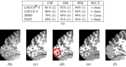
Considering tissue segmentation only, we quantitatively compare our method denoted by LOCUSB -T to the recently proposed method LOCUS--T [25] and to two well known tissue segmentation tools, FAST [31] from FSL and SPM5 [2]. The table in Figure 3 (a) shows the results of the evaluation performed on the eight BrainWeb phantoms. The mean Dice metric over all eight experiments and for all tissues is 86% for SPM5, 88% for FAST and 89% for LOCUS-T and LOCUSB-T. The mean computation times for the full 3-D segmentation were 4min for LOCUS-T and LOCUSB-T, 8min for FAST and more than 10min for SPM5. Figure 3 (b) to (f) shows the results on a real image.
Our method shows very satisfying robustness to noise and intensity nonuniformity. On Brain-Web images, it performs better than SPM5 and similarly than LOCUS-T and FAST, for a low computational time. On real 3T scans, LOCUS-T and SPM5 also give in general satisfying results. 5.4.3. Joint tissue and structure segmentation
We then evaluate the performance of the joint tissue and structure segmentation. We consider two cases: our combined approach with fixed registration parameters (LOCUSB-TS) and with estimated registration parameters (LOCUSB-TSR). For the joint tissue and structure model (LOCUSB-TS) we introduce a priori knowledge based on the Harvard-Oxford subcortical proba-bilistic atlas. FLIRT was used to affine-register the atlas. For LOCUSB-TSR, the global registration parameters RGare computed as in LOCUSB-TS as a pre-processing step. The other local
regis-tration parameters are updated at each iteration of the algorithm. Table 1 shows the evaluation on BrainWeb images using our reference segmentation of three structures. The table shows the means and standard deviations of the Dice coefficient values obtained for the eight BrainWeb images. It also shows the means and standard deviations of the relative improvements between the two models LOCUSB-TS and LOCUSB-TSR. In particular, a significant improvement of 23% is observed for the caudate nucleus. For LOCUSB-TSR, the mean computational time is of 10min for our three structures (45min for 17 structures) including the initial global registration
(RG) step using FLIRT. For comparison, on one of the brainweb phantoms, the 5% noise, 40%
nonuniformity image, Freesurfer leads respectively to 88%, 86%, 90%, with a computational time larger than 20 hours for 37 structures, while the results with LOCUSB-TSR on this phantom were 91%, 95% and 94%.
The BrainWeb database evaluation shows that the segmentation quality is very stable when the noise and inhomogeneity levels vary and this is one of the major difference with the algorithm in [25]. The three structures segmentations improve when registration is combined. In particular, in LOCUSB-TS the initial global registration of the caudate is largely sub-optimal but it is then corrected in LOCUSB-TSR. More generally, for the three structures we observe a stable gain for all noise and inhomogeneity levels.
Figure 4 shows the results obtained with LOCUSB-T, and LOCUSB-TSR on a real 3T brain scan. The structures emphasized in image (c) are the two lateral ventriculars (blue), the caudate nuclei (red) , the putamens (green) and the thalamus (yellow). Figure 4 (e) shows in addition a 3D reconstruction of 17 structures segmented with LOCUSB-TSR. The results with LOCUSB-TS are not shown because the differences with LOCUSB-TSR were not visible using this paper graphical resolution.
We observe therefore the gain in combining tissue and structure segmentation in particular through the improvement of tissue segmentation for areas corresponding to structures such as the putamens and thalamus. The additional integration of a registration parameter estimation step also provides some significant improvement. It allows an adaptive correction of the initial global registration parameters and a better registration of the atlas locally. These results could be however certainly further improved if a priori knowledge (through H(R)) on the typical deformations for each structure was used to guide these local deformations more precisely.
CSF GM WM M.C.T. LOCUSB-T 80 % (2) 92% (1) 94% (1) ≈ 4min LOCUS-T 80% (2) 92% (1) 94% (1) ≈ 4min SPM5 79% (3) 89% (4) 90% (3) ≈ 12min FAST 80% (1) 91% (1) 94% (1) ≈ 8min (a) (b) (c) (d) (e) (f)
FIGURE3. Tissue segmentation only. Table (a): mean Dice metric and mean computational time (M.C.T) values on BrainWeb over 8 experiments for different values of noise (3%, 5%, 7%, 9%) and nonuniformity (20%, 40% ). The corresponding standard deviations are shown in parenthesis. Images (c) to (f): segmentations respectively by LOCUSB-T (our approach), LOCUS-T, SPM5 and FAST of a highly nonuniform real 3T image (b). The circle in (d) points out a segmentation error which does not appear in (c).
Structure LOCUSB-TS LOCUSB-TSR Relative Improvement Left Thalamus 91% (0) 94% (1) 4% (1) Left Putamen 90% (1) 95% (0) 6% (1) Left Caudate 74% (0) 91% (1) 23% (1)
TABLE1. Mean Dice coefficient values obtained on three structures using LOCUSB-TS and LOCUSB-TSR for BrainWeb images, over 8 experiments for different values of noise (3%, 5%, 7%, 9%) and nonuniformity (20%, 40%). The corresponding standard deviations are shown in parenthesis. The second column shows the results when registration is done as a pre-processing step (LOCUSB-TS ). The third columns shows the results with our full model including iterative estimation of the registration parameters (LOCUSB-TSR). The last column shows the relative Dice coefficient improvement for each structure.
(a) (b)
(c) (d)
(e)
FIGURE4. Evaluation of LOCUSB-TSR on a real 3T brain scan (a). For comparison the tissue segmentation obtained with LOCUSB-T is given in (b). The results obtained with LOCUSB-TSR are shown in the second line. Major differences between tissue segmentations (images (b) and (d)) are pointed out using arrows. Image (e) shows the corresponding 3D reconstruction of 17 structures segmented using LOCUSB-TSR. The names of the left structures (use symmetry for the right structures) are indicated in the image.
6. Discussion
The strength of our Bayesian joint model comes from its specification via a coherently linked system of conditional models. The whole consistent treatment and tractability of the resulting coupled clustering tasks is made possible using Generalized Alternating Minimization procedures that generalize the standard EM framework. It follows an approach made of steps that are easy to interpret and that could be enriched with additional information. These modelling abilities are illustrated on a challenging real data issue of segmenting both tissues and structures from MRI brain scans. The results obtained with our cooperative clustering approach are very satisfying and compare favorably with other existing methods. The possibility to add a conditional MRF model for the intensity distribution parameters allows to handle local estimations for robustness to nonuniformities. However, further possible investigations relate to the interpolation step that we add to increase robustness to nonuniformities at a voxel level. We believe this stage could be generalized and incorporated in the model by considering successively various degrees of locality, mimicking a multiresolution approach and refining from coarse partitions of the entire volume to finer ones. Also, our choice of prior for the intensity distribution parameters was guided by the need to define appropriate conditional specifications p(ψk
c|ψN (c)k(ν) )in (28) that lead to a valid
Markov model for theψk’s. Nevertheless, incompatible conditional specifications can still be
used for inference, eg. in a Gibbs sampler or ICM algorithm with some valid justification (see [16] or the discussion in [1]). In applications, one may found that having a joint distribution is less important than incorporating information from other variables such as typical interactions. In that sense, conditional modeling allows enormous flexibility in dealing with practical problems. However, it is not clear when incompatibility of conditional distributions is an issue in practice and the theoretical properties of the procedures in this case are largely unknown and should be investigated. The tissue and structure models are also conditional MRF’s that are linked and capture several level of interactions. They incorporate 1) spatial dependencies between voxels for robustness to noise, 2) relationships between tissue and structure labels for cooperative aspects and 3) a priori anatomical information (atlas). In most approaches, atlas registration is performed globally on the entire brain resulting in structure segmentation performance that depends crucially on the accuracy of this global registration step. Our method has the advantage of providing a way to incorporate atlas registration and to refine it locally.
More generally, the framework we propose can be adapted to other applications. It provides a strategy and guidelines to deal with complex joint processes involving more than one identified sub-processes. It is based on the idea that defining conditional models is usually more straightforward and captures more explicitly cooperative aspects, including cooperation with external knowledge. The Bayesian formulation provides additional flexibility such as the possibility to deal, in a well based manner, with some sort of non-stationarity in the parameters (as the one due to intensity nonuniformities in our MRI example). Of course, depending on the application in mind, more complex energy functions than the one given in our MRI illustration may be necessary. In particular, for our example it was enough to consider separately cooperation between label sets and spatial interactions. However, one useful extension to be investigated in future work, would be to add a spatial component in the cooperation mechanisms themselves. We describe in the Appendix a possible way to perform that.