Model analysis of the factors regulating the trends and variability of carbon monoxide between 1988 and 1997

(1)

HAL Id: hal-00304168

https://hal.archives-ouvertes.fr/hal-00304168

Submitted on 20 May 2008

HAL is a multi-disciplinary open access

archive for the deposit and dissemination of sci-entific research documents, whether they are pub-lished or not. The documents may come from teaching and research institutions in France or abroad, or from public or private research centers.

L’archive ouverte pluridisciplinaire HAL, est destinée au dépôt et à la diffusion de documents scientifiques de niveau recherche, publiés ou non, émanant des établissements d’enseignement et de recherche français ou étrangers, des laboratoires publics ou privés.

Model analysis of the factors regulating the trends and

variability of carbon monoxide between 1988 and 1997

B. N. Duncan, J. A. Logan

To cite this version:

B. N. Duncan, J. A. Logan. Model analysis of the factors regulating the trends and variability of carbon monoxide between 1988 and 1997. Atmospheric Chemistry and Physics Discussions, European Geosciences Union, 2008, 8 (3), pp.9099-9138. �hal-00304168�

(2)

ACPD

8, 9099–9138, 2008 Analysis of trends and variability of carbon monoxide B. N. Duncan and J. A. Logan Title Page Abstract Introduction Conclusions References Tables Figures ◭ ◮ ◭ ◮ Back Close

Full Screen / Esc

Printer-friendly Version Interactive Discussion

Atmos. Chem. Phys. Discuss., 8, 9099–9138, 2008 www.atmos-chem-phys-discuss.net/8/9099/2008/ © Author(s) 2008. This work is distributed under the Creative Commons Attribution 3.0 License.

Atmospheric Chemistry and Physics Discussions

Model analysis of the factors regulating

the trends and variability of carbon

monoxide between 1988 and 1997

B. N. Duncan1,2and J. A. Logan3 1

Goddard Earth Sciences and Technology Center, University of Maryland at Baltimore County, Baltimore, MD, USA

2

NASA Goddard Space Flight Center, Code 613.3, Greenbelt, MD, USA

3

School of Engineering and Applied Sciences, Harvard University, Cambridge, MA, USA Received: 9 April 2008 – Accepted: 11 April 2008 – Published: 20 May 2008

Correspondence to: B. N. Duncan (bryan.n.duncan@nasa.gov)

(3)

ACPD

Full Screen / Esc

Printer-friendly Version Interactive Discussion Abstract

We used a 3-D model of chemistry and transport to investigate trends and variability in tropospheric carbon monoxide (CO) for 1988–1997 caused by changes in the overhead ozone column, fossil fuel emissions, biomass burning emissions, methane, and trans-port. We found that the decreasing CO burden in the northern extra-tropics (−0.85%/y)

5

was more heavily influenced by the decrease in European emissions during our study period than by the similar increase in Asian emissions, as transport pathways from Europe favored accumulation at higher latitudes in winter and spring. However, the opposite trends in the CO burdens from these two source regions counterbalanced at lower latitudes. Elsewhere, the factors influencing CO often compete, diminishing their

10

cumulative impact, and trends in model CO were small or insignificant for our study period, except in the tropics in boreal fall (1.1%/y), a result of emissions from major fires in Indonesia late in 1997. There was a decrease in the ozone column during the study period as a result of the phase of the solar cycle and the eruption of Pinatubo in 1991. This decrease contributed negatively to the trend in model CO by increasing the

15

hydroxyl radical (OH). The impact of this negative contribution was diminished by a pos-itive contribution of similar magnitude from increasing methane. However, the trends in these two factors did not cancel for tropospheric OH, which responded primarily to changes in the ozone column.

1 Introduction

20

The oxidizing capacity of the troposphere depends on trends and variability in carbon monoxide (CO), the main sink for the hydroxyl radical (OH) which is the primary tro-pospheric oxidant. In this study we explore the causes of trends (or lack thereof) of CO for 1988–1997. There were relatively large trends in fossil fuel emissions of CO in Asia and Europe during this period, as well as several large biomass burning events

25

(4)

ACPD

Full Screen / Esc

of Mt. Pinatubo in 1991 caused variations in tropospheric OH and subsequently CO for a few years. We deconvolve the impacts on CO of trends in fossil fuel emissions, biomass burning, methane concentrations, and the ozone column with a series of sen-sitivity simulations using the tropospheric 3-D chemistry and transport model (CTM) described in Duncan et al. (2007).

5

During the 1980s and 1990s there was an expansion of the routine measurements of CO, especially surface observations from the flask sampling program of the National Oceanic and Atmospheric Administration (NOAA) Earth System Research Laboratory, Global Monitoring Division (GMD) (Novelli et al., 1992). The total column of CO is also measured at several locations around the world, with data collected at a few sites since

10

the 1970s (Zander et al., 1989; Yurganov et al., 1997; Mahieu et al., 1997; Zhao et al., 2000; Rinsland et al., 1998; Rinsland et al., 1999; Rinsland et al., 2000). This database provides the means with which to derive trends in observed CO and to evaluate model performance.

There were few systematic measurements of CO before the late 1980s. The data

15

suggest that CO was increasing at about 1%/y in the Northern Hemisphere (NH) (Khalil and Rasmussen, 1988; Zander et al., 1989; Yurganov et al., 1999), probably because of increasing anthropogenic emissions (Novelli et al., 1998). By the end of the 1980s, this upward trend was replaced by a downward trend (Khalil and Rasmussen, 1994; Novelli et al., 1994). There were sparse measurements in the Southern Hemisphere

20

(SH) before the 1990s. Surface data from Cape Point, South Africa, suggest no trend for 1979–1987 (Brunke et al., 1990).

Novelli et al. (2003) reported that global surface CO decreased by 0.52 ppbv/y be-tween 1991 and 2001, with ∼30% of that decline being attributed to the aftermath of the eruption of Mt. Pinatubo (June 1991), and the subsequent increase in tropospheric

25

OH (Bekki et al., 1994; Novelli et al., 1994; Dlugokencky et al., 1996; Dlugokencky et al., 1998). The remainder of the decline was caused by the decrease in anthropogenic emissions in the NH, where CO decreased by 1.4 ppbv/y in the northern extra-tropics. Novelli et al. (2003) found no significant trend in the SH, though there was IAV

(5)

associ-ACPD

Full Screen / Esc

ated with variations in biomass burning emissions.

We describe briefly the formulation and evaluation of the model in Sect. 2; further details are given in Duncan et al. (2007). In Sect. 3, we discuss the trends in the dom-inant factors with the potential to influence trends in CO and OH (i.e., overhead ozone column, fossil fuel emissions, biomass burning emissions, transport and methane). In

5

Sect. 4, we present the trends in model CO. In Sect. 5, we analyze the causes of CO trends and variability. A summary of our results is given in Sect. 6.

2 Model and simulation description

2.1 Model framework

In our earlier paper (Duncan et al., 2007) we described and evaluated the version of

10

the GEOS-Chem CTM that we use here, so we only provide a brief description. The model is driven by assimilated meteorological data, capturing variations in CO caused by IAV in transport. The model captures feedbacks between CO and OH by using a chemical parameterization scheme that allows OH to respond to changes in the concentrations of trace gases, meteorology, and the overhead ozone column (Duncan

15

et al., 2000). We use the merged data set of Stolarski and Firth (2006) to account for IAV in the ozone column. It is derived from measurements by the Total Ozone Mapping Spectrometer/Solar Backscatter Ultraviolet (TOMS/SBUV) instruments.

The sources of CO include direct emissions from biomass burning, fossil fuel and biofuel combustion, and chemical production from the oxidation of methane and

bio-20

genic and anthropogenic non-methane hydrocarbons (NMHC). The annual variations in emissions from fossil fuel combustion are based on national inventories where available and on statistics for liquid fuel use (Bey et al., 2001a; Duncan et al., 2007). The total annual biomass burned inventory used in this study is described in Lobert et al. (1999), with CO emissions summarized in Duncan et al. (2003a); the IAV in biomass burning

25

(6)

ACPD

Full Screen / Esc

are described by Yevich et al. (2003). We account for the production of CO from the oxidation of methane assuming a yield of 1 CO per methane oxidized as discussed in Duncan et al. (2007). The production of CO from NMHC is estimated by converting the emissions of NMHC to CO by applying a yield of CO per NMHC oxidized as rec-ommended by Altshuller (1991). Uncertainties in the budget of CO for 1988–1997 are

5

discussed in Duncan et al. (2007).

We used version 5.02 of the GEOS-Chem model for transport (http://www-as. harvard.edu/chemistry/trop). The transport is driven by assimilated meteorology from the Goddard Earth Observing System Global Modeling and Assimilation Office (GEOS GMAO) (Schubert et al., 1993; Takacs et al., 1994). We use GEOS-1 fields from

10

January 1988 to November 1995, and GEOS-Strat fields from December 1995 to De-cember 1997. The sigma vertical levels of the model are given in Bey et al. (2001a). All meteorological data were regridded from a resolution of 2◦×2.5◦(latitude by longitude) to 4◦

× 5◦.

2.2 Model simulations

15

We discuss seven simulations. The first is our Standard run and the second tracks CO tracers tagged as a function of their source: both are described in Duncan et al. (2007). We use the other simulations to quantify the contributions from trends in the ozone column, fossil fuel emissions, biomass burning emissions, transport, and methane to trends in CO and in OH in the Standard simulation. In each, we fix one of these factors

20

to its values for 1988 for the entire simulation, while allowing the others to vary. 2.3 Model evaluation

A detailed evaluation of model CO with observations is presented in Duncan et al. (2007). We compared model CO to observations from the NOAA/GMD flask sam-pling program, CO column observations, and profiles from various aircraft campaigns.

25

(7)

ACPD

Full Screen / Esc

CO are reproduced well by the model implying that the magnitude and timing of the emissions are reasonable. The model reproduces the 20% decrease in CO observed at high NH latitudes 1988–1997 and the 10% decrease in the North Pacific, caused primarily by a decrease in European emissions as discussed below. The model is too low at the seasonal maximum in spring in the southern tropics, except for locations in

5

the Atlantic Ocean. This problem may be caused by an overestimate of the frequency of tropical deep convection, as discussed in Duncan et al. (2007).

3 Trends in causal factors

3.1 Fossil fuel emissions

There were strong regional trends in fossil fuel emissions for 1988-1997 as shown in

10

Fig. 2 of Duncan et al. (2007). Table 1 presents the emissions for fossil fuels by region for several years. European emissions decreased 39% from 1988 to 1997, from 148 Tg to 90 Tg CO. Emissions in Western Europe decreased by 33% (61 Tg to 41 Tg), mostly through regulatory controls, while in Eastern Europe (>22◦E) they decreased by 45% (87 Tg to 48 Tg) because of the economic contraction following the breakup of the

for-15

mer Soviet Union. At the same time, the countries of East Asia, especially China, un-derwent an unprecedented economic expansion, increasing emissions by 52% (102 Tg to 155 Tg). The decrease in emissions from North America was smaller, 16% (111 Tg to 93 Tg). The decrease of emissions in Europe, −58 Tg, was approximately counter-balanced by the increase in emissions from East Asia, +53 Tg. Overall total fossil fuel

20

emissions from the NH decreased only by 6%, or 23 Tg CO, for 1988–1997, despite the strong regional trends.

3.2 Overhead ozone column

Figure 1 shows the deviation (%) of the monthly mean ozone column from the monthly means for 1979–2006 using the merged data set of Stolarski and Firth (2006). During

(8)

ACPD

Full Screen / Esc

our study period, 1988–1997, the ozone column was strongly impacted by the eruption of Mt. Pinatubo in June 1991 (WMO, 2007). Substantial ozone loss occurred after the eruption of Mt. Pinatubo, especially in the NH mid-latitudes. Hydrolysis of N2O5on

sul-fate aerosols in the lower stratosphere effectively sequestered NO allowing enhanced catalytic destruction of ozone by chlorine (Mickley et al., 1997). The ozone column also

5

depends on natural sources of variability, including the solar cycle and quasi-biennial oscillation (QBO).

We calculate trends in ozone with the multivariate linear regression model of Ziemke et al. (1997). Such regression models include terms for the solar cycle and QBO, so that they can compute trends attributable to changes in chlorine and bromine. Here,

10

however, we are interested in the actual trend in ozone which impacts tropospheric OH and, subsequently, CO, so we omit the dependence of ozone on the solar cycle and the QBO. There are significant downward trends in all seasons for all four zonal bands for 1988-1997 as shown in Fig. 1. Our study period begins near the peak of a solar cycle and ends near a minimum (e.g., sunspot activity in Fig. 1 as a proxy), and much

15

of the trend in the tropics is caused by the dependence of ozone on the solar cycle. 3.3 Biomass burning emissions

Duncan et al. (2003a) found that there were no large-scale trends in biomass burning in the tropics/subtropics for the 1980s and 1990s, but there was significant IAV. Wotawa et al. (2001) found that 63% of the IAV of summertime CO above 30◦N can be

ex-20

plained by IAV in boreal forest fires in the high, NH latitudes. Biomass burning is highly seasonal, with some episodic and sometimes extreme events that occur in regions with high biomass loads (i.e., boreal forests and Indonesian forests underlain by peat). The boreal forests of North America experienced unusually large fires in 1994 and 1995, and Indonesia experienced fires in 1991, 1994, and 1997; those in 1997 were

particu-25

larly severe, releasing an estimated 130 Tg CO (Duncan et al., 2003a; Duncan et al., 2003b).

(9)

ACPD

Full Screen / Esc

3.4 Methane

The source of CO from methane oxidation is about one-third of the total source of CO (e.g., Holloway et al., 2000; Duncan et al., 2007). Dlugokencky et al. (1998) derived an average trend in the global methane burden of 8.9±0.1 ppbv/y for 1984– 1996 from GMD surface observations growth, with a decrease in the growth rate

5

of 0.9±0.1 ppbv/y. We use the GMD measurements to give annually and zonally-averaged mixing ratios for four zonal bands of equal area in the model. The trends in methane are similar in each band for 1988–1997, about +0.4%/y.

3.5 Transport

Changes in atmospheric circulation caused by the El Ni ˜no/Southern Oscillation (ENSO)

10

can be substantial, impacting many regions of the world (Lau and Yang, 2002). Our study period includes the most extreme ENSO event of the century that occurred in 1997–1998 (Bell and Halpert, 1998; Glantz, 2001) and the weaker, prolonged ENSO event of 1990—1995 (Allan and D’Arrigo, 1999). Only two periods, 1988-early 1989 and early 1996, experienced La Ni ˜na conditions, with the 1996 event being weak. By

15

chance, our study period began with an unusually strong La Ni ˜na and ended with an unusually strong El Ni ˜no.

In the extra-tropics of the NH, the North Atlantic Oscillation (NAO) is one of the domi-nant influences on climate variability from eastern North America to Siberia, especially during winter (Hurrell et al., 2002). Duncan and Bey (2004) showed that IAV of the

20

NAO caused variations in surface CO over Europe, effectively masking the influence of the downward trend in European fossil fuel emissions for 1987–1997.

3.6 Other factors

Trends and variability in emissions of NO_x and NMHC, and in tropospheric ozone may impact OH and hence CO. As discussed in Duncan et al. (2007), we use the

(10)

ACPD

Full Screen / Esc

averaged distributions (1988–1997) from the GEOS-Chem simulation with the kinetic solver presented in Duncan and Bey (2004) as input to this simulation which uses the parameterization method to calculate OH. These fields, and subsequently their impact on OH, already account for variations of transport, emissions, the overhead ozone columns, etc.

5

We use a linear scaling of the direct emissions of CO to account for CO from the oxidation of anthropogenic NMHC (Duncan et al., 2007), so this source of CO is not an independent cause of variability in our simulation. We estimate the production of CO from biogenic NMHC oxidation, which is a function of temperature, sunlight, and/or NO_x as described in Duncan et al. (2007); this source of CO varies annually by 6%

10

during the study period (or by less than 1% of the total CO source).

The use of the two meteorological fields may contribute a spurious component to any calculated trend even though the model versions are similar (except for the num-ber of levels in the stratosphere). Therefore, we show trends for both 1988–1997 and 1988–1995 in Sect. 5, but our conclusions are not dependent on the ending year of

15

our analysis. Any spurious components are dwarfed because of real variations in the causal factors described in Sects. 3.1–3.5, which explain the majority (>80%) of varia-tion in the total CO trends (see Sect. 5).

4 Trends in model CO

We discuss the burden and trends in model CO for four latitude bands: 30–90◦N (HNH,

20

high NH), 0◦–30◦N (TNH, tropical and subtropical NH), 0◦–30◦S (TSH), and 30–90◦S (HSH). Although there is heterogeneity within each band, the factors that influence the distributions and trends are different enough to warrant this artificial demarcation. Except in the extra-tropics in winter, the lifetime of CO is typically short in relation to meridional mixing so that a trend in one of our zonal bands may not necessarily affect

25

the trend in another (Khalil and Rasmussen, 1994). Unless otherwise specified, we compute trends using the method presented in Ziemke et al. (1997).

(11)

ACPD

Full Screen / Esc

Figure 2 shows the tropospheric burden of CO by source (i.e., methane oxidation, fossil fuels and biofuels, biomass burning, and biogenic NMHC oxidation) for 1988– 1997. The production of CO from methane oxidation is ∼35% of the total tropospheric source and contributes a similar fraction, about 100–120 Tg CO, to the total burden. The global burden from biomass burning shows two peaks each year associated with

5

the timing of the burning in the tropics of the NH and SH. The contribution of biomass burning to the burden in the HNH reflects transport from the tropics and subtropics, as the extratropical source peaks in summer. The burden from fossil fuels peaks in late boreal winter/early spring in this region, and is similar in magnitude to the burden from biomass burning at that time. The burden from the oxidation of biogenic NMHC is the

10

smallest contributor overall in the HNH, but is ∼60% of the fossil fuel burden in boreal summer.

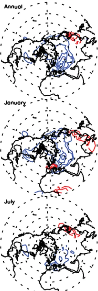
Figure 3 shows the spatial trends in the distribution of the model surface CO (ppbv/y) for 1988–1997 for the NH. (Annual trends were calculated for each surface grid box using monthly means, using y=A+Bx and minimizing the Chi-square error statistic.)

15

There are strong downward annual trends that maximize over Russia (<−10 ppbv/y) and strong upward trends in East Asia (2–10 ppbv/y). The annual trends are more heavily weighted to the trends in winter than summer because of wintertime accumu-lation of CO. There are positive trends in surface CO in January over Western Europe despite the strong decrease in emissions there (Table 1); this trend occurs because the

20

last two winters of our study period were predominately in the negative phase of the NAO as discussed by Duncan and Bey (2004). Over most of the tropics and SH (not shown) there are no significant trends in surface CO greater than ±1 ppbv/y, except there is an upward trend in Southeast Asia, over the Bay of Bengal, and over northern Africa near the equator. The trends at 500 hPa are mostly not significant (not shown).

25

Figure 4 shows the trends in the tropospheric CO burden of the Standard simula-tion. The seasonal and annual trends in the HNH are all negative (−0.5 to −1.1%/y); the largest negative trend occurs in March–May. Overall, the HNH has the largest seasonal and annual trends. The seasonal trends in the tropical bands show

(12)

consid-ACPD

Full Screen / Esc

erable variability (−0.7 to 1.4%/y) though the annual trends are not significant in the TNH and are only 0.3%/y in the TSH. The largest positive trends occur in the tropics in September–November. The smallest trends occur in the HSH.

5 Analysis of causes of CO trends and variability

Figure 5 shows the effect on the CO burden of the four main factors influencing trends

5

and IAV: biomass burning, methane, fossil fuels, and the ozone column. For each sim-ulation we fix one of these factors to its values for 1988 for the entire simsim-ulation, while allowing the others to vary. The figure shows the monthly deviation of the CO burden (∆CO) in each sensitivity simulation, defined as the monthly burden in the Standard simulation minus the monthly burden in the sensitivity simulation. Interannual variation

10

in biomass burning is the main driver of large-scale, episodic variability in the trop-ics, especially related to major burning events in Indonesia in 1991, 1994, and 1997. In contrast, the upward trend in global methane contributed a monotonic increase in CO. The downward trend in fossil fuels emissions contributed a steady, but seasonally-varying, decrease in the HNH. The changes in the ozone column caused an overall

15

decrease, though with variability.

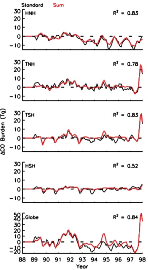
Figure 6 shows ∆CO in the Standard simulation and the sum of ∆CO from the four sensitivity simulations in Fig. 5. There are nonlinear feedbacks between CO, methane, and OH, so that the components of the total trend caused by the causal factors will not necessarily sum to the total CO trend in the Standard case. Nevertheless, the

20

figure shows that these four causal factors explain the majority of CO variability globally (R2=0.84) for 1988–1997 and in the HNH, TNH, and TSH (0.78–0.83). However, only about half is explained in the HSH (R2_{=0.52). Our sensitivity simulation where we fix} the transport for each year to that in 1988 shows that transport explains much of the remaining variability in the HSH. This result is not surprising for the HSH as most of

25

(13)

ACPD

Full Screen / Esc

5.1 Impact of regional trends in fossil fuel emissions

The net change in NH fossil emissions is small (Table 1), although there are large regional changes in emissions and in trends in surface CO (Fig. 3). Figure 7 shows the trends in the CO burden for the Standard run and for the simulation with fossil fuel emissions fixed to 1988 levels. The negative trends in the Standard simulation in the

5

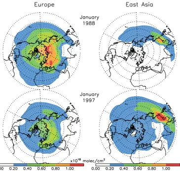
HNH become insignificant or less negative in the sensitivity run. However, the trends in the TNH are similar for both simulations. The decrease in European emissions is the primary cause of the decrease in the CO burden at higher latitudes, but the effect of the decrease in CO from Europe on CO at lower latitudes is offset by the increase in CO from Asia as illustrated in Fig. 8, which shows the total column burden of CO from

10

Asian and European sources in January of 1988 and 1997.

The CO burden in the NH, especially in the HNH, is more heavily influenced by the decrease in European emissions than by the similar increase in Asian emissions for two reasons. First, pollution from Europe is emitted at higher latitudes (40◦–65◦N) than that from North America (30◦–45◦N) and from East Asia (20◦–40◦N, but mainly

15

30◦_–40◦_{N). The average lifetime of CO increases with latitude, particularly in winter}

when CO behaves like an inert tracer at high latitudes. Second, in winter, much of the export of pollution from Europe occurs near the surface towards Russia and the Arctic (Duncan and Bey, 2004), while some CO from East Asia is transported to the southwest over Indochina and the Bay of Bengal (Newell and Evans, 2000; Bey et al.,

20

2001b; Stohl et al., 2002; Liu et al., 2003) into a region where its lifetime is less than a month. These transport pathways are evident in Fig. 8. The annual emissions of CO from Europe in 1988 are similar to those from Asia in 1997 (Table 1), but the greater hemispheric impact of European CO in 1988 is clear in Fig. 8. As a result, the decrease in the CO burden from European sources (−1.8 Tg/y) is larger in magnitude than the

25

increase in the burden from Asian sources (+1.1 Tg/y) as shown in Fig. 9. The overall burden of CO from fossil fuels in the NH decreases by 8% while emissions change by 6%.

(14)

ACPD

Full Screen / Esc

We used tagged tracer simulations to examine the contributions of regional trends in fossil fuel emissions at GMD stations that are downwind of major source regions (Fig. 10). The decrease in model CO at Barrow, Alaska (−2.8 ppbv/y), is mostly due to CO from European fossil fuel emissions (−3.4 ppbv/y), and agrees well with the ob-served trend (−3.2 ppbv/y). The burdens from East Asian and North American sources

5

are much smaller than that from Europe in 1988, but by 1997 all three are of more sim-ilar magnitude. The model captures the seasonality of the trend, largest in winter and spring, with the greatest effect of European sources during these seasons (Fig. 11). European pollution plays less of a role in determining the overall trend at lower latitudes, but the decrease in European CO is evident, including at Tae-ahn, Korea (−2.2 ppbv/y),

10

Cape Meares (−1.1 ppbv/y), and Midway (−1.1 ppbv/y) in Fig. 10. The effect of the de-crease in European sources for 1988–1997 is offset by the inde-crease in East Asian fossil fuel emissions at most of the midlatitude sites (e.g., Bermuda, Midway). Slightly neg-ative or insignificant trends in CO from North American sources occur at the stations, even at Bermuda which is typically impacted by the outflow of North America, reflecting

15

the relatively weaker decrease in emissions (Table 1). 5.2 Methane and overhead ozone columns

The trends in the simulation where the overhead ozone columns were fixed to 1988 lev-els are less negative than those in the Standard simulation, as shown in Fig. 12. The observed decrease in the ozone columns for 1988–1997 contributed a negative

com-20

ponent to the CO trend in the Standard case by enhancing CO loss through reaction with OH. On the other hand, the observed increase in methane contributed a posi-tive component as it led to an increase in the source of CO from methane oxidation (Fig. 12).

The compensating nature of the observed trends in column ozone and methane on

25

CO trends (Fig. 5) is fortuitous for our study period. The trends in the ozone column depend, in part, on the solar cycle, leading to an increase in OH in 1988–1997, but the 11-y solar cycle should contribute a regular cyclic component to the trend in OH

(15)

ACPD

Full Screen / Esc

and hence in CO. Consequently, the trend in methane (should it increase again) and the cycle in the overhead ozone column may alternate from canceling each other to reinforcing each other in their effects on CO trends.

The observed trends in column ozone and methane did not have a compensating effect on OH (Fig. 13). Clearly, model OH is sensitive to changes in the overhead

5

ozone column in the tropics year-round (±4%) and in the middle and high latitudes in local summer (±5%). In the HNH and HSH, there is significant IAV in OH which will prejudice any trend; two deviations in OH in the HNH in 1993 and 1995 are associated with strong negative deviations in the overhead ozone column (Fig. 1). In contrast, the trend in methane has little impact on OH (Fig. 13) as reaction with methane is not the

10

primary sink for OH.

The trends in OH in the Standard run are positive in the tropical bands in all seasons for 1988–1995, but are not significant for 1988–1997 for the TSH and for September-February in the TNH (Fig. 14). As will be discussed in Sect. 5.5, the component of the upward trend in OH from the decreasing ozone columns is partially offset by the loss

15

of OH through reaction with CO from the Indonesian fires. 5.3 Episodic high-impact events

Trends are particularly sensitive to extreme events near the start or end of the time series being considered. Novelli et al. (2003) estimated that the global trend in surface CO for 1991–2001 (−0.52 ppbv/y) would be −1.5 ppbv/y if data from 1997 to

mid-20

1999 were removed from the calculation; abnormally large emissions of CO occurred in 1997 and 1998 from wildfires in Indonesia (late 1997, early 1998), the boreal forests (in 1998), and Mexico (in 1998), perturbing the tropospheric CO burden by 16% on average for almost 3 years.

It is apparent from Fig. 5 that including or excluding 1997 in our analysis will impact

25

the calculated trends, especially in the tropics. Figure 15 shows the seasonal and annual trends in the Standard simulation and the sensitivity simulation with the biomass burning emissions fixed to 1988 levels. The seasonal trends are similar in both runs

(16)

ACPD

Full Screen / Esc

for all seasons, except September–November when the Indonesia fires occurred. The positive trends in the TNH and TSH in the Standard run are negative or not significant in the sensitivity simulation.

There is not a major response of the model CO burden to the aftermath of the Mt. Pinatubo eruption in June 1991 (Fig. 5). Model calculations in the literature

in-5

dicate that OH initially decreased during the first year following the eruption because of the scattering effects of sulfate aerosols, which reduced the amount of UV radia-tion in the troposphere (Dlugokencky et al., 1996), and began to increase in 1992 and 1993 as the ozone column decreased in 1992/1993 (Fig. 1; Bekki et al., 1994). We do not include the scattering effects of stratospheric sulfate aerosols on photolysis rates.

10

However, Fuglestvedt et al. (1994) found the response of methane was damped as the largest changes in the column occurred outside of the tropics and in winter (Fig. 1). 5.4 Transport

The sensitivity simulation, where we fix transport fields throughout the simulation to those of 1988, does not provide useful information on the causes of CO trends as

15

1988 began in a weak El Ni ˜no and ended in a strong La Ni ˜na. Thus the natural tran-sition between the ENSO phases is broken by repeating 1988 meteorology, possibly introducing a spurious forcing to this sensitivity simulation.

5.5 Contributions of causal factors to trends in model OH

The hydroxyl radical is sensitive to a number of factors (e.g., Spivakovsky et al, 2000),

20

especially to changes in the ozone column (see Fig. 13) and to changes in CO itself, as about 60% of the sink of OH is through reaction with CO. Global mean OH in our simulation is ∼0.9×106molec/cm3(Duncan et al., 2007). Figure 16 shows the monthly-average OH with the monthly mean (1988–1997) removed. Globally, model OH varies ±10% about the mean for 1988–1997. Interannual variability in OH of this magnitude

25

(17)

ACPD

Full Screen / Esc

(Bousquet et al., 2005; Prinn et al., 2005).

Figure 14 shows that the seasonal OH trends in the Standard run for 1988–1997 in all four zonal bands are not significant, except in NH spring and summer (<0.5%/y) and the HSH in September–November (−0.5%/y). The component of the trend in OH associated with trends in the ozone column is important in the tropics year-round and

5

in the high latitudes in local spring and summer, as shown in Fig. 13. The component of the OH trend in the tropics due to biomass burning is approximately counter-balanced by that due to the overhead ozone column in September–November. Biomass burning caused decreases in OH as high as 10% during the 1997 Indonesian fires in the tropics. The influence of fossil fuels is comparatively weak, except in the HNH; the decrease in

10

CO from fossil fuels impacts OH predominately in spring, when CO is seasonally high, and early summer (±2%; Fig. 13), when OH is seasonally high. The impact of the trend in methane is small as noted above.

6 Summary

We presented a comprehensive analysis of the causes of the trends and interannual

15

variability of tropospheric CO for 1988–1997. The northern extra-tropics experienced a downward trend in the CO burden in all seasons, highest in winter (−1.3 Tg/y) and spring (−1.5 Tg/y), associated with the downward trend in fossil fuel emissions from Europe. The higher latitudes responded strongly to the decrease in European sources, but not to the similar increase in Asian sources, as the former are emitted further north

20

and transport pathways favor accumulation at higher latitudes in winter and spring. However, the opposite trends in the CO burdens from these two source regions coun-terbalanced at lower latitudes.

A monotonic increase in methane between 1988 and 1997 contributed positively to CO, but the concurrent decrease in the ozone column and concomitant increase in

25

OH caused a compensating decrease in CO. Consequently, the annual trends in CO in the tropics and southern extra-tropics were small (0.25 Tg/y) or insignificant. The

(18)

ACPD

Full Screen / Esc

decrease in the ozone column in the tropics resulted from our study period beginning near a maximum in the solar cycle and ending near a minimum, and the solar cycle causes an 11 year cycle in OH on longer time scales. Should methane increase in the future, components of the CO trend from methane oxidation and the ozone column may alternate between canceling and reinforcing one another.

5

Two large events occurred during our study period, but only one impacted CO trends significantly. The Indonesian wildfires in late 1997 released a tremendous amount of CO over about 3 months. Consequently, the trends in tropical CO were high (0.7– 1.1 Tg/y) in September–November. The trend in the southern extra-tropics (0.6 Tg/y) was also affected by transport of CO from this event. Although large fires also occurred

10

in Indonesia in 1991 and 1994, they had far less impact on trends, but they impacted IAV of CO considerably. The second large event, the eruption of Mt. Pinatubo had a relatively small impact on OH, and subsequently CO, as it occurred during the middle of our study period and the largest decreases in the ozone columns occurred at high latitudes in winter when OH is seasonally low.

15

The increases in model OH were significant in spring and summer in the north-ern extra-tropics, and were associated with the decrease in the ozone column and in European CO sources. In the southern extra-tropics, the OH trends were primarily in-fluenced by the decrease in the ozone columns. The trends in OH for 1988–1995 were positive in all regions, but the 1997 Indonesian wildfires strongly influenced the tropical

20

trends for 1988–1997, effectively negating the impact of decreasing ozone columns. The trends in model OH were weak or not significant and there was large variability, ±10% about the mean, for 1988–1997. These findings are in general agreement with other studies, which inferred trends in OH from observations of methyl chloroform and

14

CO (Bousquet et al., 2005; Manning et al., 2005; Prinn et al., 2005).

25

Acknowledgements. B. Duncan gratefully acknowledges important discussions with Stacey

Frith on trends in column ozone and thanks Jerry Ziemke for guidance on the calculation of trends. This research was supported by NASA Grant NAG-1-2307 (B. Duncan) and by the National Science Foundation grant ATM-0554804 to Harvard University (J. Logan).

(19)

ACPD

Full Screen / Esc

Printer-friendly Version Interactive Discussion References

Allan, R. J. and D’Arrigo, R. D.: Persistent ENSO sequences: How unusual was the 1990–1995 El Ni ˜no?, Holocene, 9(1), 101–118, 1999.

Altshuller, P.: The production of carbon monoxide by the homogeneous NO_x-induced photoox-idation of volatile organic compounds in the troposphere, J. Atmos. Chem., 13, 155–182,

5

1991.

Bekki, S., Law, K. S., and Pyle, J.A.: Effect of ozone depletion on atmospheric methane and CO concentrations, Nature, 371, 595–597, 1994.

Bell, G. D., and Halpert, M. S.: Climate Assessment for 1997, Bull. Am. Meteorol. Soc., 79, S1–S50, 1998.

10

Bey, I., Jacob, D. J., Yantosca, R. M., et al.: Global modeling of tropospheric chemistry with assimilated meteorology: Model description and evaluation, J. Geophys. Res., 106, 23 073– 23 095, 2001a.

Bey, I., Jacob, D. J., Logan, J. A., and Yantosca, R. M.: Asian chemical outflow to the Pacific: Origins, pathways and budgets, J. Geophys. Res., 106, 23 097–23 113, 2001b.

15

Bousquet, P., Hauglustaine, D. A., Peylin, P., Carouge, C., and Ciais, P.: Two decades of OH variability as inferred by an inversion of atmospheric transport and chemistry of methyl chlo-roform, Atmos. Chem. Phys., 5, 2635–2656, 2005,

http://www.atmos-chem-phys.net/5/2635/2005/.

Brunke, E.-G., Scheel, H. E., and Seiler, W.: Trends of tropospheric CO, N₂O and methane as

20

observed at Cape Point, South Africa, Atmos. Environ., 24A, 585–595, 1990.

Chameides, W. L., Liu, S. C., and Cicerone, R. J.: Possible variations in atmospheric methane, J. Geophys. Res., 82, 1795–1798, 1977.

Dlugokencky, E. J., Dutton, E. G., Novelli, P. C., Tans, P. P., Masarie, K. A., Lantz, K. O., and Madronich, S.: Changes in methane and CO growth rates after the eruption of Mt. Pinatubo

25

and their link with changes in tropical tropospheric UV flux, Geophys. Res. Lett., 23, 2761– 2764, 1996.

Dlugokencky, E. J., Masarie, K. A., Lang, P. M., and Tans, P. P.: Continuing decline in the growth rate of atmospheric methane burden, Nature, 393, 447–450, 1998.

Duncan, B. N., Portman, D., Bey, I., and Spivakovsky, C. M.: Parameterization of OH for efficient

30

computation in chemical tracer models, J. Geophys. Res., 105, 12 259–12 262, 2000. Duncan, B. N., Martin, R. V., Staudt, A. C., Yevich, R. M., and Logan, J. A.: Interannual and

(20)

ACPD

Full Screen / Esc

Seasonal Variability of Biomass Burning Emissions Constrained by Satellite Observations, J. Geophys. Res., 108, D2, 4040, doi:10.1029/2002JD002378, 2003a.

Duncan, B. N., Bey, I., Chin, M., Mickley, L. J., Fairlie, T. D., Martin, R. V., and Matsueda, H.: Indonesian Wildfires of 1997: Impact on Tropospheric Chemistry, J. Geophys. Res., 108, D15, 4458, doi:10.1029/2002JD003195, 2003b.

5

Duncan, B. N. and Bey, I.: A Modeling Study of the Export Pathways of Pollution from Eu-rope: Seasonal and Interannual Variations (1987–1997), J. Geophys. Res., 109, D08301, doi:10.1029/2003JD004079, 2004.

Duncan, B. N., Logan, J. A., Bey, I., Megretskaia, I. A., Yantosca, R. M., Novelli, P. C., Jones, N. B., and Rinsland, C. P.: Global budget of CO, 1988–1997: Source estimates and

valida-10

tion with a global model, J. Geophys. Res., 112, D22, D22301, doi:10.1029/2007JD008459, 2007.

Fuglestvedt, J. S., Jonson, J. E., and Isaksen, I. S. A.: Effects in reductions in stratospheric ozone on tropospheric chemistry through changes in photolysis rates, Tellus, 46B, 172–192, 1994.

15

Glantz, M. H.: Currents of Change, Impacts of El Ni ˜no and La Ni ˜na on Climate and Society, 84–100, Cambridge Univ. Press, New York, 2001.

Hurrell, J. W. and Folland, C. K.: A change in the summer atmospheric circulation over the North Atlantic, in Exchanges: Selected Research Papers, vol. 7, Clim. Variability and Predict., World Clim. Res. Progr., Southampton, UK, 2002.

20

Khalil, M. A. K. and Rasmussen, R. A.: Carbon monoxide in the Earth’s atmosphere: Indications of a global increase, Nature, 332, 242–245, 1988.

Khalil, M. A. K. and Rasmussen, R. A.: Global decrease in atmospheric carbon monoxide concentration, Nature, 370, 639–641, 1994.

Lau, K.-M. and Yang, S.: Walker circulation, in Encyclopedia of Atmospheric Sciences, edited

25

by J. Holton, J. P. Pyle, and J. Curry, 2505–2509, Academic, San Diego, Calif., 2002. Liu, H., Jacob, D. J., Bey, I., Yantosca, R. M., and Duncan B. N.: Transport pathways for Asian

pollution outflow over the Pacific: Interannual and seasonal variations, J. Geophys. Res., 108 D20, 8786, doi:10.1029/2002JD003102, 2003.

Lobert, J., Keen, W., Logan, J., and Yevich, R.: Global chlorine emissions from biomass

burn-30

ing: Reactive chlorine emissions inventory, J. Geophys. Res., 104, 8373–8389, 1999. Mahieu, E., Zander, R., Delbouille, L., Demoulin, P., Roland, G., and Servais, C.: Observed

(21)

ACPD

Full Screen / Esc

recorded at the Jungfraujoch, J. Atmos. Chem., 28, 227–243, 1997.

Manning, M. R., Lowe, D. C., Moss, R. C., Bodeker, G. E., and Allan, W.: Short-term variations in the oxidizing power of the atmosphere, Nature, 436, doi:10.1038/nature03900, 2005. Mickley, L. J., Abbatt, J. P. D., Frederick, J. E., and Russell III, J. M.: Response of

summer-time odd nitrogen and ozone at 17 mbar to Mount Pinatubo aerosol over the southern

mid-5

latitudes: Observations from the Halogen Occultation Experiment, J. Geophys. Res., 102, 23 573–23 582, 1997.

Newell, R. E. and Evans, M. J.: Seasonal changes in pollutant transport to the North Pacific: the relative importance of Asian and European sources, Geophys. Res. Lett., 27, 2509–2512, 2000.

10

Novelli, P. C., Steele, L. P., and Tans, P. P.: Mixing ratios of carbon monoxide in the troposphere, J. Geophys. Res., 102, 12 855–12 861, 1992.

Novelli, P. C., Masarie, K. A., Tans, P. P., and Lang, P. M.: Recent changes in atmospheric carbon monoxide, Science, 263, 1587–1590, 1994.

Novelli, P. C., Masarie, K. A., and Lang, P. M.: Distributions and recent changes in carbon

15

monoxide in the lower troposphere, J. Geophys. Res., 103, 19 015–19 033, 1998.

Novelli, P. C., Masarie, K. A., Lang, P. M., Hall, B. D., Myers, R. C., and Elkins, J. W.: Reanalysis of tropospheric CO trends: Effects of the 1997–1998 wildfires, J. Geophys. Res., 108(D15), 4464, doi:10.1029/2002JD003031, 2003.

Prinn, R., Huang, J., Weiss, R. F., et al.: Evidence for variability of atmospheric hydroxyl radicals

20

over the past quarter century, Geophys. Res. Lett., 32, L07809, doi:10.1029/2004GL022228, 2005.

Rinsland, C. P., Jones, N. B., Connor, B. J., et al.: Northern and southern hemisphere ground-based infrared spectroscopic measurements of tropospheric carbon monoxide and ethane, J. Geophys. Res., 103(D21), 28 197–28 218, doi:10.1029/98JD02515, 1998.

25

Rinsland, C. P., Goldman, A., Murcray, F. J., et al.: Infrared solar spectroscopic measurements of free tropospheric CO, C₂H₆, and HCN above Mauna Loa, Hawaii: Seasonal variations and evidence for enhanced emissions from the Southeast Asian tropical fires of 1997–1998, J. Geophys. Res., 104(D15), 18 667–18 680, 10.1029/1999JD900366, 1999.

Rinsland, C. P., Mahieu, E., Zander, R., Demoulin, P., Forrer, J., and Buchmann, B.: Free

30

tropospheric CO, C₂H₆, and HCN above central Europe: Recent measurements from the Jungfraujoch station including the detection of elevated columns during 1998, J. Geophys. Res., 105, 24 235–24 249, 2000.

(22)

ACPD

Full Screen / Esc

Schubert, S. D., Rood, R. B., and Pfaendtner, J.: An assimilated data set for earth science applications, Bull. Amer. Meteorol. Soc., 74, 2331–2342, 1993.

Spivakovsky, C. M., Logan, J. A., Montzka, S. A., Balkanski, Y. J., Foremen-Fowler, M., Jones, D. B. A., Horowitz, L. W., Brenninkmeijer, C. A. M., Prather, M. J., Wofsy, S. C., and McElroy, M. B.: Three dimensional climatological distribution of tropospheric OH: update and

evalua-5

tion, J. Geophys. Res., 105, 8931–8980, 2000.

Stohl, A., Eckhardt, S., Forster, C., James, P., and Spichtinger, N.: On the path-ways and timescales of intercontinental air pollution transport, J. Geophys. Res., 107, doi:10.1029/2001JD001396, 2002.

Stolarski, R. S. and Frith, S. M.: Search for evidence of trend slow-down in the long-term

10

TOMS/SBUV total ozone data record: the importance of instrument drift uncertainty, Atmos. Chem. Phys. 6, 4057–4065, 2006.

Sze, N. D.: Anthropogenic CO emissions: implications fro the atmospheric CO-OH-methane cycle, Science, 195, 673–675, 1977.

Takacs, L. L., Molod, A., and Wang, T.: Documentation of the Goddard Earth Observing System

15

(GEOS) General Circulation Model–Version 1, NASA Technical Memorandum 104606, 1, 1994.

Thompson, A. M., and Cicerone, R. J.: Possible perturbations to atmospheric CO, methane, and OH, J. Geophys. Res., 91, 10 853–10 864, 1986.

WMO (World Meteorological Organization): Scientific Assessment of Ozone Depletion: 2006,

20

Global Ozone Research and Monitoring Project – Report No. 50, 572 pp., Geneva, Switzer-land, 2007.

Yevich, R. and Logan, J. A.: An assessment of biofuel use and burning of agricultural waste in the developing world, Global Biogeochem. Cyc., 17, 4, 1095, doi:10.1029/2002GB001952, 2003.

25

Yurganov, L. N., Grechko, E. I., and Dzhola, A. V.: Variations of carbon monoxide density in the total atmospheric column over Russia between 1970 and 1995: Upward trend and disturbances, attributed to the influence of volcanic aerosol and forest fires, Geophys. Res. Lett., 24, 1231–1234, 1997.

Yurganov, L. N., Grechko, E. I., and Dzhola, A. V.: Zvenigorod carbon monoxide total column

30

time series: 27 yr of measurements, Chemosphere, 1, 127–136, 1999.

Zander, R., Demoulin, Ph., Ehhalt, D. H., Schmidt, U., and Rinsland, C. P.: Secular increase of the total vertical column abundance of carbon monoxide above central Europe since 1950,

(23)

ACPD

Full Screen / Esc

J. Geophys. Res., 94, 11 021–11 028, 1989.

Zhao, Y., Kondo, Y., Murcray, F. J., Liu, X., Koike, M., Irie, H., Strong, K., Suzuki, K., Sera, M., and Ikegami, Y.: Seasonal variations of HCN over northern Japan measured by ground-based infrared solar spectroscopy, Geophys. Res. Lett., 27, 14, 2085–2088, 2000.

Ziemke, J. R., Chandra, S., McPeters, R. D., and Newman, P. A.: Dynamical proxies of column

5

ozone with applications to global trend models, J. Geophys. Res., 102, D5, 6117–6129, 1997.

(24)

ACPD

Full Screen / Esc

Printer-friendly Version Interactive Discussion Table 1. Direct emissions (Tg CO) from fossil fuel sources by region.

Year Europe1 North America2 East Asia3 Sum Emissions 88 148 111 102 361 92 120 96 125 341 97 90 93 155 338 ∆Emissions 97–88 ₋₅₈ ₋₁₈ +53 −23 Ratio 97/88 0.61 0.84 1.52 0.94 1 38◦N–70◦N; 15◦W–78◦E and 52◦N–70◦N; 75◦ E–180◦. 2 28◦N–70◦N; 170◦W–50◦W.38◦N–44◦N; 75◦E–150◦E.

(25)

ACPD

Full Screen / Esc

Printer-friendly Version Interactive Discussion Fig. 1.

(26)

ACPD

Full Screen / Esc

Printer-friendly Version Interactive Discussion Fig. 1. The top four panels show the change in the observed O₃ column (%) for 1979–2006

relative to the monthly mean column for 1979–2006 for four zonal bands. The time period of our study, 1988–1997, is shown between red vertical lines; the annual and seasonal ob-served trends (%/y) are shown at right. The trends have the effects of the seasonal cycle re-moved. DJF=December–February; MAM=March–May; JJA=June–August; SON=September– November; ANN=January–December. The bottom panel shows the monthly number of sunspots/month for 1979–2006, a proxy for the solar cycle.

(27)

ACPD

Full Screen / Esc

Printer-friendly Version Interactive Discussion 0 20 40 60 80 100 120 140 HNH 0 20 40 60 80 100 120 TNH 0 20 40 60 80 100 120 Tg CO TSH 0 20 40 60 80 HSH 88 89 90 91 92 93 94 95 96 97 98 Year 0 100 200 300 400 GLOBE Total Biomass Burning Biogenic NMHC Ox Fossil Fuel & Biofuel

CH

4 Ox (dashed)

(28)

ACPD

Full Screen / Esc

Printer-friendly Version Interactive Discussion Trends in surface CO (ppbv/y) for 1988-1997 (top). Downward trends are shown as

Fig. 3. Trends in surface CO (ppbv/y) for 1988–1997 (top). Downward trends are shown as

blue lines, upward trends as red lines, and no trend as green lines with contour spacing of −21, −18, −15, −12, −9, −6, −3, 0, 3, 6, 9, 12, 15, 18, and 21. January trends (middle) with contour spacing of −50, −40, −30, −20, −10, −5, 0, 5, 10, 20, 30, 40, and 50. July trends (bottom) with the same contour spacing as the top panel.

(29)

ACPD

Full Screen / Esc

The seasonal and annual trends for the CO burden (%/y, Tg/y) in the Standard

Fig. 4. The seasonal and annual trends for the CO burden (%/y, Tg/y) in the Standard

(30)

ACPD

Full Screen / Esc

Δ

Fig. 5. The deviation of the monthly CO burden (∆CO; Tg) for each sensitivity simulation

defined as the monthly CO burden for the Standard simulation minus the monthly burden of the sensitivity simulation.

(31)

ACPD

Full Screen / Esc

The same as Figure 5, except for the Standard simulation (black). The red line

Fig. 6. The same as Fig. 5, except for the Standard simulation (black). The red line represents

(32)

ACPD

Full Screen / Esc

The seasonal and annual trends for the CO burden (Tg/y) in the standard and fossil

Fig. 7. The seasonal and annual trends for the CO burden (Tg/y) in the standard and fossil fuel

(33)

ACPD

Full Screen / Esc

Figure 8. Total column burdens of CO (Tg) from fossil fuel emissions from Europe and East

Fig. 8. Total column burdens of CO (Tg) from fossil fuel emissions from Europe and East Asia

(34)

ACPD

Full Screen / Esc

Printer-friendly Version Interactive Discussion Fig. 9. Monthly tropospheric burden of CO (Tg) in the NH from Europe (black), North America

(35)

ACPD

Full Screen / Esc

Figure 10. Surface CO (black line with dots) observed at several NOAA/GMD stations. The

Fig. 10. Surface CO (black line with dots) observed at several NOAA/GMD stations. The red

line represents total model CO in the Standard run. CO from fossil fuel emissions from Europe, East Asia, and North America are shown as green, magenta, and blue lines, respectively. The sum of all three fossil fuel tracers is shown in pale blue.

(36)

ACPD

Full Screen / Esc

Printer-friendly Version Interactive Discussion Fig. 11. (top) Trends (ppbv/y) for the model and observed CO at the NOAA/GMD station

in Barrow, Alaska. (bottom) Trends for tagged tracers from three industrialized regions; two standard deviations are shown by the vertical lines.

(37)

ACPD

Full Screen / Esc

The seasonal and annual trends for the CO burden (Tg/y) for the standard and two

Fig. 12. The seasonal and annual trends for the CO burden (Tg/y) for the standard and two

(38)

ACPD

Full Screen / Esc

Printer-friendly Version Interactive Discussion Fig. 13. Same as Fig. 5, except for model OH.

(39)

ACPD

Full Screen / Esc

Trends (%/y) for model OH in the Standard simulation; two standard deviations are

Fig. 14. Trends (%/y) for model OH in the Standard simulation; two standard deviations are

(40)

ACPD

Full Screen / Esc

Printer-friendly Version Interactive Discussion Fig. 15. The seasonal and annual trends for the CO burden (Tg/y) in the standard and biomass

(41)

ACPD

Full Screen / Esc

Figure 16. Monthly OH with the monthly mean OH for 1988-1997 removed.