HAL Id: hal-00136929
https://hal.archives-ouvertes.fr/hal-00136929
Preprint submitted on 15 Mar 2007
HAL is a multi-disciplinary open access
archive for the deposit and dissemination of
sci-entific research documents, whether they are
pub-lished or not. The documents may come from
teaching and research institutions in France or
abroad, or from public or private research centers.
L’archive ouverte pluridisciplinaire HAL, est
destinée au dépôt et à la diffusion de documents
scientifiques de niveau recherche, publiés ou non,
émanant des établissements d’enseignement et de
recherche français ou étrangers, des laboratoires
publics ou privés.
The forbidden 1082 nm line of sulphur: the photospheric
abundance of sulphur in the Sun and 3D effects
Elisabetta Caffau, Hans-Guenter Ludwig
To cite this version:
Elisabetta Caffau, Hans-Guenter Ludwig. The forbidden 1082 nm line of sulphur: the photospheric
abundance of sulphur in the Sun and 3D effects. 2007. �hal-00136929�
hal-00136929, version 1 - 15 Mar 2007
(DOI: will be inserted by hand later)
c
ESO 2007
Astrophysics
&
The forbidden 1082 nm line of sulphur:
the photospheric abundance of sulphur in the Sun and 3D effects
E. Caffau
1; H.-G. Ludwig
2,11 Observatoire de Paris-Meudon, GEPI, 92195 Meudon Cedex, France, 2 CIFIST Marie Curie Excellence Team
Received ...; Accepted ...
ABSTRACT
Context.Sulphur is an element which is formed in the α-process and is easily measured in the gaseous phase in external galaxies. Since it does not form dust, it is the preferred indicator for α-elements, rather than Si or Mg, for which dust corrections are necessary. The measurement of the sulphur abundance in stars is not an easy task, relying mainly on high excitation lines with non-negligible deviations from LTE. The 1082 nm sulphur forbidden transition is less sensitive to departures from LTE and is less dependent on temperature uncertainties than other sulphur lines usually employed as abundance indicators. Therefore it should provide a more robust abundance diagnostics.
Aims.To derive the solar photospheric abundance of sulphur from the 1082 nm [SI] line and to investigate 3D effects present in G- and F-type atmospheres at solar and lower metallicity.
Methods.High-resolution, high signal-to-noise solar intensity and flux spectra were used to measure the sulphur abundance from the [SI] 1082 nm line. CO5BOLD hydrodynamical model atmospheres were applied to predict 3D abundance corrections for the [SI] line.
Results.The solar sulphur abundance is derived to be 7.15 ± (0.01)stat±(0.05)sys, where the statistical uncertainty represents the scatter in the
determination using four different solar spectra and the systematic uncertainty is due to the modelling of the blending lines. Sulphur abundances obtained from this line are insensitive to the micro-turbulence. 3D abundance corrections, found from strictly differential comparisons between 1D and 3D models, are negligible in the Sun, but become sizable for more metal-poor dwarfs.
Key words.Sun: abundances – Stars: abundances – Hydrodynamics
1. Introduction
Weak forbidden lines arising from the ground level of an ion in the dominant ionisation stage can be extremely useful for measuring abundances. They are often unaffected by depar-tures from LTE, and they are insensitive to the atmospheric temperature uncertainties as well as micro-turbulence. On the other hand, forbidden lines are sensitive to gravity, but this is of no concern in our analysis, since the solar gravity is well known. The most widely used of such forbidden lines is cer-tainly the 630 nm [OI] line, which has often been the oxygen abundance indicator of choice, even though it is blended with a Ni line, which, in the solar spectrum, contributes about 1/3 of the equivalent width (EW) of the feature. Recently, Ryde (2006) has used the corresponding forbidden line of sulphur at 1082 nm, to measure the sulphur abundance in a sample of
Send offprint requests to: Elisabetta.Caffau@obspm.fr
stars in the Galactic disc. However, he did not investigate the line in the solar spectrum. The [SI] 1082 nm line is clearly vis-ible in solar spectra; we therefore decided to measure the solar sulphur abundance from this line and to compare this measure-ment to values obtained from other sulphur lines. We further investigated 3D effects influencing the [SI] line with the help of CO5BOLD hydrodynamical model atmospheres for the Sun as well as for a few metal-poor G- and F-type stars.
To our knowledge, the first published analysis of the [SI] 1082 nm line in the Sun was carried out by Swensson (1968a), who related the transition 3p4 3P2—3p4 1D2 of S , to a
feature with an observed wavelength of 1082.12 nm that ap-peared next to a Cr line at 1082.164 nm and a telluric H2O
line at 1082.215 nm. This identification was later confirmed by Swensson (1968b). He estimated an EW of 0.35 pm (in Swensson 1968a) and of 0.40±0.05 pm (in Swensson 1968b) in
2 Caffau et al.: [SI] line at 1082 nm
the solar observed intensity spectrum of Delbouille & Roland (1963).
Independently, Swings et al. (1969) identified the 1082 nm [SI] line in improved tracings of the solar spectrum and they published a convincing detection of the solar [SI] line and solar sulphur abundance based on this line. They measured the EW in the two spectra and found 0.32 ± 0.02 pm (from the Jungfraujoch solar intensity spectrum) and 0.36 ± 0.03 pm (from the solar scan of Kitt Peak), from which they derived a sulphur abundance of 7.24 and 7.30, respectively, by adopting a log g f of –8.61. Using one-dimensional model atmospheres they predicted an EW of 0.30 pm for the [SI] line at solar disc centre, for an assumed solar sulphur abundance of 7.21 (Lambert & Warner 1968). This prediction is in good agree-ment with their two measureagree-ments.
2. Models and atomic data
S is the dominant ionisation stage in the atmospheres consid-ered in this paper. The [SI] line arises from the ground level, so that the abundance of sulphur is fairly directly measured, instead of measuring the abundance from an excited level rep-resenting a small fraction of the total population.
For the [SI] line we adopted a laboratory wave-length 1082.1176 nm (in air) and a log g f of –8.617 (see http://physics.nist.gov/PhysRefData/ADS). Our analy-sis is based on 3D model atmospheres computed with the CO5BOLD code (Wedemeyer et al. 2003). More de-tails about the models used can be found in Caffau et al. (2007, in preparation). In addition to the CO5BOLD hydrodynamical simulations we used several 1D mod-els. The spectral synthesis codes employed are Linfor3D (see http://www.aip.de/∼mst/Linfor3D/linfor 3D manual.pdf) for all models and SYNTHE (Kurucz 2005) for the Holweger-M¨uller model. The 1D models we used are briefly described hereafter:
1. An “internal 1D” model generated by Linfor3D; this is a 1D atmospheric structure computed by horizontal and tem-poral averaging of a 3D model structure over surfaces of equal (Rosseland) optical depth. These 1D models provide estimates of the influence of fluctuations around the mean stratification on the line formation process. Comparing 3D and internal 1D models of this kind is largely independent of arbitrary input parameters, the micro-turbulence being the only free parameter.
2. In correspondence to each 3D CO5BOLD model we constructed hydrostatic 1D model atmospheres computed with the LHD code. LHD is a Lagrangian 1D (assum-ing plane-parallel geometry) hydrodynamical model atmo-sphere code. It employs the same micro-physics (equation-of-state, opacities) as CO5BOLD. The convective energy transport is described by mixing-length theory. The spatial discretisation of the radiative transfer equation is similar
to the one in CO5BOLD, albeit simplified for the 1D ge-ometry. A flux-constant hydrostatic stratification including radiative and convective energy transport processes is ob-tained by following the actual thermal and dynamical evo-lution of the atmosphere until a stationary state is reached. LHD produces standard 1D model atmospheres which are differentially comparable to corresponding CO5BOLD models. Remaining choices entering an LHD model calcu-lation are the value of the mixing-length parameter, which formulation of mixing-length theory to use, and in what way turbulent pressure is treated in the momentum equa-tion. Note, that these degrees of freedom are also present in other 1D model atmosphere codes.
3. A 1D solar model computed by F. Castelli with version 9 of the ATLAS code and the solar abundances of Asplund et al. (2005) available at http://wwwuser.oats.inaf.it/castelli/sun/ ap00t5777g44377k1asp.dat
4. The Holweger-M¨uller solar model (Holweger 1967; Holweger & M¨uller 1974).
A 3D CO5BOLD model constitutes a statistical realisation of the atmospheric flow field over a certain period of time. For spectral synthesis purposes, the state of the flow is sampled at equal intervals in time. We informally refer to a flow sample as a “snapshot”. Each snapshot represents the stellar photosphere at a particular instant of time. Besides the 3D model construc-tion as such, 3D spectral synthesis also uses up quite a lot of computer time. The computing time increases linearly with the total number of snapshots Nt. Hence, Ntshould be restricted to
as small a number as possible, but chosen carefully to obtain a statistically meaningful result. We like to emphasise that the strength of a line is usually a less critical feature than its de-tailed line shape or line shift for which the velocity field plays an important role.
Table 1 summarises the atmospheric parameters and snap-shot selection we did for our 3D models. Where possible, we tried to cover several convective turn-over timescales in the sur-face layers (in the Sun approximately 500 s). The sampling in-terval was chosen not to be an integer fraction of the period of the dominant oscillation mode of the computational box, which is closely related to the period at which most power is expected for stellar five-minute like oscillations. This ensures that one does not always sample the oscillations at the same phase, which would lead to a bias in the statistical properties of the velocity field controlling line broadening and line shifts. Moreover, we selected our snapshots to ensure that the statistics of the sub-sample closely followed the statistics of the whole ensemble, e.g., in terms of the resulting effective temperature and fluctuations around it.
Table 1 also lists a characteristic timescale tc = HP/c
(HP: pressure scale height at τross = 1, c: sound speed), half
the (isothermal) acoustic cut-off period. From hydrodynamical models spanning a large range in effective temperature, gravity, and metallicity Svensson & Ludwig (2005) found that the
evo-Table 1. The CO5BOLD models considered in this research. The first three columns list the atmospheric parameters of the models, the fourth column the number of snapshots Nt
con-sidered, the last-but-one column the time interval covered by the selected snapshots, and the last column a characteristic timescale tcof the evolution of the granular flow.
Teff log g [Fe/H] Nt time tc
(K) (cm s−2) (s) (s) 5770 4.44 0.0 25 6000 17.8 6500 4.00 0.0 28 16800 49.6 5770 4.44 –2.0 1 80 15.2 6250 4.50 –2.0 10 9600 15.9 5900 4.50 –3.0 19 9500 15.6 6500 4.50 –3.0 12 2400 16.0
lutionary timescale of surface granulation roughly scales with
tc. Hence, considering tcone can relate an intrinsic timescale
of the atmosphere to the total time (column “time” in Table 1) over which the evolution of a relaxed model was followed.
As is obvious from Table 1, the model with parameters 5770K/4.44/-2.0 does not fulfil the statistical criteria for the snapshot selection we outlined before. However, since the line strength does not vary strongly over the evolution of a 3D model we nonetheless felt that we could include this single snapshot model to obtain at least an estimate of the abundance corrections for its atmospheric parameters.
3. Data
We used two high-resolution, high signal-to-noise ratio, spec-tra of the centre disc solar intensity. These were that of Neckel & Labs (1984) (hereafter referred to as the “Neckel intensity spectrum”) and that of Delbouille, Roland, Brault, & Testerman (1981) (hereafter referred to as the “Delbouille intensity spec-trum”) (http://bass2000.obspm.fr/solar spect.php); we further used the solar flux spectrum of Neckel & Labs (1984) and the one from http://kurucz.harvard.edu/sun.html (referred to as the “Kurucz flux spectrum”).
4. Data analysis
To derive sulphur abundances in the solar spectra we measured the equivalent width (EW) and in addition fitted the line pro-files. EWs were measured using the IRAF task splot and the deblending option, since the spectral range is rather complex. The EW we obtain in this way takes into account the contri-bution of the lines which lie to the red (Cr , Fe and C2) and
to the blue (Fe and C2) of the [SI] line. For this reason our
value is considerably lower than the one found by Swings et al. (1969). However, since lines with poorly known atomic data crowd the region, we estimate an uncertainty in the EW com-putation of at least 0.03 pm, which translates into an error in
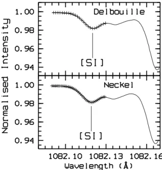
Fig. 1. The observed intensity spectra (solid line) are plotted over on the fit (crosses) obtained using a grid of synthetic spectra based on the Holweger-M¨uller model computed with SYNTHE. Delbouille refers to the Delbouille intensity spec-trum, Neckel to the Neckel intensity spectrum (see text for de-tails).
the abundance of 0.05 dex. The line profile fitting was done us-ing a code, described in Caffau et al. (2005), which performs a χ2 minimisation of the deviation between synthetic profiles and the observed spectrum. Figure 1 shows the fit of the solar intensities obtained from a grid of synthetic spectra synthesised with SYNTHE and based on the Holweger-M¨uller model.
The solar sulphur abundance derived from the [SI] line,
A(S)1=7.15±(0.01)stat±(0.05)sys, is in good agreement with the
one obtained from the 675 nm triplet in Caffau et al. (2007, sub-mitted to A&A). For the [SI] line the 3D abundance correction is small in the Sun, and independent of the micro-turbulence. The solar A(S) obtained from this line (see Table 2), which is unaffected by 3D corrections and is insensitive to NLTE effects, is believed to be close to the actual solar abundance.
As a theoretical exercise we computed 3D corrections for flux spectra in metal-poor stars. As expected, the [SI] line is not sensitive to the micro-turbulence, the 3D corrections do not depend on this parameter. The results are depicted in Fig. 2. From the plot we can deduce that for solar-metallicity stars the 3D abundance corrections are negligible. The corrections in-crease for decreasing stellar metallicity. They become sizable at [Fe/H]=–2.0 and [Fe/H]=–3.0. If we compare the average tem-perature structure of the 3D models to the 1D reference LHD models, we realise that they are very close for solar-metallicity stars (see Fig. 3). For metal-poor stellar models the 3D and 1D LHD average temperature structures are not in good
4 Caffau et al.: [SI] line at 1082 nm
Table 2. Solar sulphur abundances from the various observed spectra. Col. (1) is the wavelength of the line followed by an identification flag, D means Delbouille and N Neckel intensity spectrum, F Neckel and K Kurucz flux spectrum. Col. (2) is the Equivalent Width. Col. (3) is the sulphur abundance, A(S), according CO5BOLD 3D model. Cols. (4)-(11) are the A(S) from 1D models, even numbered cols. correspond to ξ = 1.0 km s−1, odd numbered cols. to ξ = 1.0 km s−1. Col. (12) is the A(S) from
WIDTH code. Col. (13) is the A(S) from fitting with a HM grid; col. (14) and (15) are 3D corrections with micro-turbulence of 1.5 and 1.0 km s−1, respectively.
Wave EW A(S) from EW FIT 3D-1D
nm pm 3D 1D ATLAS HM LHD WIDTH HM 1.0 1.5 1.0 1.5 1.0 1.5 1.0 1.5 1.0 1.5 (1) (2) (3) (4) (5) (6) (7) (8) (9) (10) (11) (12) (13) (14) (15) 1082D 0.212 7.140 7.140 7.139 7.154 7.153 7.170 7.170 7.123 7.122 7.150 0.0175 0.0182 1082N 0.223 7.162 7.162 7.161 7.176 7.175 7.192 7.191 7.145 7.144 7.176 0.0175 0.0182 1082F 0.258 7.138 7.148 7.147 7.173 7.172 7.180 7.179 7.137 7.135 7.133 7.168 0.0011 0.0024 1082K 0.258 7.138 7.148 7.147 7.173 7.172 7.180 7.179 7.137 7.135 7.133 7.168 0.0011 0.0024
ment. At log τ < −1, 3D models are cooler, and the difference increases towards external layers. According to the contribu-tion funccontribu-tion the [SI] line is formed mostly at log τ ≈ −1 for solar-metallicity stars, but at log τ ≈ −2 and log τ ≈ −3, for [Fe/H] of –2.0 and –3.0, respectively. The basic reason for the behaviour of the contribution function is that the continuous opacity (mostly H−) decreases for lower metallicity at fixed Rosseland optical depth in the outer atmospheric layers. The effect is more pronounced in 3D models due to the lowering of the average temperature at low metallicity. Since the line emerges from a transition from the ground level, the popula-tion of the line’s lower level is not very sensitive to the abso-lute temperature, so that temperature differences between 3D and 1D models are not so important. However, the tempera-ture gradients also differ markedly between 3D and 1D models in the line-forming layers. In the weak line approximation, the line strength is proportional to the gradient of the (log) source function on the continuum optical depth scale, so EWs com-puted with the 3D model with a steeper temperature gradient tend to be larger than the ones from a 1D model. In comparison to 1D a lower sulphur abundance is needed in a 3D model to obtain the same equivalent width of the line, corresponding to a negative 3D abundance correction.
For metal-poor F-type stars contributions due to horizontal fluctuations (3D-1D internal) are about one third of the overall abundance corrections, while for metal-poor G-type stars this contribution is negligible. Horizontal temperature fluctuations in metal-poor photospheres are significantly smaller in G-type than in F-type atmospheres. The reason does not lie so much in a different level of the convective dynamics between the two spectral types. The reason is related to the temperature attained due to the cooling by convective overshooting. In G-type stars photospheric temperatures become so low that H2 molecular
formation sets in. This drives up the specific heat, leading to smaller changes of the temperature in response to pressure dis-turbances induced by overshooting motions. As evident from
Fig. 2. 3D abundance corrections: each correction is located ac-cording the parameters (Teff and [Fe/H]) of the related model; the models have very similar gravity (log g in between 4.44 and 4.50). Black numbers depict the 3D-1D LHD differences, grey (green in colour) ones the 3D-1D internal model differences.
Fig. 2, the “demarcation line”, where this effect becomes im-portant, is located around Teff≈6000 K for dwarf stars.
5. Discussion
Our analysis implies that the [SI] line constitutes a robust in-dicator of the sulphur abundance, in spite of the fact that the measurement of EW is affected by a rather large error. Our A(S)=7.15 ± (0.01)stat±(0.05)sys is consistent with the value
provided by Lodders (2003), A(S)=7.21 ± 0.05.
It is of some interest to consider the 3D corrections for this line. A 3D model atmosphere differs from a 1D one in essen-tially two respects. In the first place, a hydrodynamical simu-lation provides a mean temperature structure which is different from that of a 1D atmosphere assuming radiative equilibrium; this is illustrated in Fig. 3. In the second place, the hydrody-namical simulation takes into account the effects of
horizon--4 -3 -2 -1 0 1 log10 τ 4 6 8 10 12 T [kK] 3D 1D LHD [Fe/H]=0.0 [Fe/H]=-3.0
Fig. 3. Average temperature structures of 3D CO5BOLD (solid lines) in comparison to 1D LHD (dotted lines) models. The lower pair of curves is for 5770K/4.44/0.0 (solar) models, the upper pair for 5900K/4.50/-3.0 models. For clarity, the later models were shifted by +2000 K.
tal temperature fluctuations, which is something a 1D model cannot do. Bearing this in mind it is fairly easy to understand the meaning of the two values for the correction provided in Fig. 2. The 3D-1D corrections (grey/green in the plot) is the difference between the 3D model and the internal 1D model, which is the average of the 3D model over surfaces of equal (Rosseland) optical depth. Therefore, this correction provides information about the influence of the horizontal fluctuations on the derived abundance. As suggested from the figure, this correction increases as the effective temperature increases, but it is always very small when compared to the global correction. The 3D-1D LHD model correction (black in the plot) takes into account both the different mean structure of the two models, as well as the horizontal fluctuations. The LHD model, that em-ploys the same micro-physics (equation-of-state, opacities) as CO5BOLD, provides a better estimate of the “3D effects” than the use of other 1D model atmospheres (e.g. ATLAS models). The effects of different assumptions about the micro-physics may result in a cancellation or enhancement of the effects, which are related to the different nature of the 3D model.
For the Sun the 3D abundance corrections are negligible. For metal-poor stars the full 3D corrections become sizable, the sulphur abundance is lowered by a factor of 1.6, and they are dominated by effects related to the mean temperature profile, rather than by that of the horizontal fluctuations. Due to the lack of available models we cannot give 3D corrections for slightly metal-poor stars yet, but we intend to do so as soon as we have these models at hand.
Acknowledgements. The authors wish to thank Rosanna Faraggiana
and Piercarlo Bonifacio for their help and suggestions with this re-search. The authors acknowledge gratefully financial support from EU contract MEXT-CT-2004-014265 (CIFIST).
References
Asplund, M., Grevesse, N., & Sauval, A. J. 2005, ASP Conf. Ser. 336: Cosmic Abundances as Records of Stellar Evolution and Nucleosynthesis, 336, 25
Caffau, E., Bonifacio, P., Faraggiana, R., Franc¸ois, P., Gratton, R. G., & Barbieri, M. 2005, A&A, 441, 533
Delbouille, L., & Roland, G. 1963, Liege, 1963. Holweger, H. 1967, Zeitschrift f¨ur Astrophysik, 65, 365 Holweger, H., & Mueller, E. A. 1974, Sol. Phys., 39, 19 Lambert, D. L., & Warner, B. 1968, MNRAS, 138, 181 Kurucz, R. L. 2005, Memorie della Societ`a Astronomica
Italiana Supplement, 8, 14 Lodders, K. 2003, ApJ, 591, 1220
Neckel, H., & Labs, D. 1984, Sol. Phys., 90, 205 Ryde, N. 2006, A&A, 455, L13
F. Svensson & H.-G. Ludwig, 2005, in : Proceedings of “The 13th Cambridge Workshop on Cool Stars, Stellar Systems and the Sun”, eds. F. Favata, G.A.J. Hussain, B. Battrick, p. 979
Swensson, J. W. 1968, Zeitschrift f¨ur Astrophysik, 68, 151 Swensson, J. W. 1968, Astrophys. Lett., 1, 185
Swings, J. P., Lambert, D. L., & Grevesse, N. 1969, Sol. Phys., 6, 3
Wedemeyer, S., Freytag, B., Steffen, M., Ludwig, H.-G., & Holweger, H. 2003, Astronomische Nachrichten, 324, 410