Computational Approaches to Stochastic Vehicle
Routing Problems
Dimitris J. Bertsimas
Philippe Chervi
Michael Peterson
WP# 3285-91-MSA
April 18, 1991
Computational Approaches to Stochastic Vehicle Routing
Problems
Dimitris Bertsimas
Philippe Chervit
Michael Peterson
April 18, 1991
Abstract
We develop and test several heuristics for two well-known vehicle routing problems which have stochastic demand: the probabilistic traveling salesman problem (PTSP) and the prob-abilistic vehicle routing problem (PVRP). The goal in these problems is to obtain optimal a
priori tours, that is, tours which are designed before demands are known. We develop a number
of heuristics which lead to such solutions, examine the quality of these solutions, and perform computational experiments against alternative strategies of re-optimization, which we are able to compute using sampling techniques. Based on extensive testing we conclude that our heuris-tics are very close in terms of performance compared with re-optimization strategies and can be used by a practitioner.
*D. Bertsimas, Sloan School of Management, MIT. The research of D. Bertsirnas was partially supported by the National Science Foundation research initiation grant DDM-9010332 and NSF grant DDM-9014751.
t P. Chervi, Operations Research Center, MIT.
tM. Peterson, Sloan School of Management, MIT. The research of M. Peterson was partially supported by NFS graduate fellowship grants RCD-88-54827 and RCD-90-50002
1
Introduction
This paper examines two well-known and related problems in optimization under uncertainty: the probabilistic traveling salesman problem (PTSP) and the 1-vehicle probablistic vehicle routing prob-lem (PVRP). Below we give formal definitions of both probprob-lems, but more simply, these probprob-lems can be thought of as identical to their deterministic counterparts except that the demands of the points to be visited are random rather than fixed.
We shall be concerned throughout the paper with comparing what we call a priori strategies to
re-optimization strategies. An a priori strategy is one which is formulated in advance of any information
about the demands (other than their locations). In contrast, a strategy of re-optimization allows tours to be designed after demand information is known, so that each re-optimized solution is tailored to a particular realization. Of course, re-optimization, where practical, will give better solutions than
a priori strategies. However, in many practical situations, such a strategy might prove prohibitively
costly or may not be desirable for other reasons. For example, a delivery company may wish to have its drivers follow the same route each day in order to gain familiarity with a particular set of customers. Moreover, as we shall see, re-optimization solutions may have resource requirements entirely too high for smaller firms, firms which might nevertheless wish to improve operational performance.
Let us define the two problems in which we are interested. Consider a graph G(V, E) on n nodes representing locations to be visited. An instance of the PTSP is specified by a matrix D of inter-node distances together with a set of probabilities {Pi}, each pi specifying the probability that a given node i must be visited on a realization of the problem. Such a node is said to be present for that realization. In the case where pi = p for all i we have an instance of the homogeneous PTSP; otherwise we have a heterogeneous PTSP. The goal is to find an a priori tour r (i.e. a tour designed prior to any realization) to minimize the expected length
E[LT] E p(S)L(S), (1)
scv
where each Lr(S) is a tour visiting the nodes present on a given realization S in the same order as they appear in the tour r. The term p(S) is the probability of realization S and is given by
p(S) = Pi II (1 - Pi). (2)
iEs iqs
realization S, an optimal TSP tour is re-calculated. The cost under re-optimization is given by
E[ETSP] = E P(S)LTSP(S), (3)
scv
where LTSP(S) is the length of the optimal traveling salesman tour through the points of S. Al-though D may be general, in this study we focus on Euclidean distances only.
Some simple additions to the PTSP just described give us the 1-vehicle PVRP, the second problem to be examined. Consider a set of (random) demands at the n locations, a point "O" which we designate as the depot, and a single vehicle of capacity Q. We suppose that the vehicle must collect loads from the n locations, returning periodically to a depot to empty. The demands X1,.. , Xn, are independent integer random variables, each with a known probability distribution,
and the objective is to design a routing strategy to minimize expected travel distance. In order to define the problem more precisely we introduce the notation:
Q vehicle capacity
K = maximum demand value, K < Q d(i, j) _ distance between nodes i and j
s(i, j) - d(i, O) + d(O, j) - d(i,j)
= Pr{demand at node i equals j}
f(m,r) - Pr{demand for 1,...,m is r}
As with the PTSP, a strategy of re-optimization is available, though in practical situations it might be prohibitively expensive.
Two cases (which we call a and b) arise in the PRVP. In case a, the designed routes are followed exactly, so that all locations (even those having zero demand on the day) are visited. In case b, the same routes are used, but locations having zero demand are simply skipped. In both cases, the total expected distance traveled will be that of the a priori route chosen plus certain radial terms stemming from returns to the depot. More formally, let 7i denote the probability that the vehicle
exactly reaches its capacity at node i, and i the probability that the vehicle exceeds its capacity at
node i. Using our f(m, r) notation these probabilities are given by
71 = 0 (4)
i E Epif(i - l, q Q - k ) , 2<i<n, (5)
(6)
L*J K-1 K
=
z
z z
P. f(i-1 qQ-k) 2 < i < n, (7)=l k=l r=k+l
The probabilities f(m, r) can be computed from the recursion
min(K,r)
f(m,r)= yf(m Pk -1,r-k),m > 2,r < Km (8)
k=O
with the initial condition
f(l,r)=p7', O<r<K. ()
Now re-number the points 1... n so that point 1 is the first point on our a priori tour, point 2 is second, etc. Expected tour lengths are then given by
n n
E[La] = a d(i, i + 1) + Z(bis(i, i) + ys (i, i + 1)) (10)
i=O i=1
n i-1 n n
E[L] = Ed(O,i)pi p + d(i,O)pi
11
p +i=1 r=l i=1 r=i+l
n n j-1
a,
Z
d(i,j)pipjIl
P +i=1j=i+l r=i+l
E is(i,i) + 7ipjs(ij) I Pr ' (11)
i=1 j=i+l r=i+l
where Pi = 1- p, the probability of positive demand at node i, and n + 1 = 0, the depot node. The first expression consists of the underlying tour plus radial correction terms for returns to the depot. These correction terms vary according to whether capacity is exactly met or strictly exceeded. The second expression derives from the same principles, but is more complicated since zero demands may be skipped.
The PTSP was introduced and analyzed by Jaillet [13] and further explored by Bertsimas and Howell [6]. The PVRP with general demand distributions was analyzed in Bertsimas [7]. For a comprehensive survey of the area of a priori optimization see [8].
In this paper we undertake the task of performing extensive computational testing of several heuristic procedures. In particular we address the following issues
* How do simple heuristics compare to re-optimization? * At what problem size does asymptotic behavior emerge?
* What are the relative effects of more sophisticated heuristics like local improvement and dy-namic programming procedures?
* What are the relevant conclusions for the practitioner?
A novel aspect of our approach is the use of sampling techniques combined with variance reduction techniques in order to get more precise estimates. In this way we are able to compare a priori and re-optimization strategies.
All of our subsequent analysis will deal with proposing and analyzing a priori heuristic approaches for these two problems. Sections 2 and 3 do this for the PTSP, while sections 4 and 5 do this for the PVRP. Section 6 summarizes the conclusions of the paper.
2
Heuristics for the Probabilistic Traveling Salesman
Prob-lem
In this section we describe the heuristic methods we apply to the PTSP. These fall into two categories: tour construction techniques (these are typically used as the first step in our procedures), and local improvement procedures. For a more detailed discussion of the procedures, consult the references given.
2.1
The Space-filling Curve Heuristic
Spacefilling curves, first introduced by Peano, Hilbert, and Sirpinski, have more recently come into use in solving routing and partitioning problems (c.f. Bartholdi and Platzman [2], [3]). Our description here will omit most technical details.
We define a spacefilling curve to be a continuous mapping IF : C -a S where C is the unit interval and S is the unit square. The specific form of 'I will not be given here, but it has several important properties:
* is onto but not necessarily surjective. Thus any image in S has one or more pre-images in C.
* A pre-image 0 satisfying P(8G) = (, y) may be computed in O(k) operations, where k is the number of bits needed to specify the image (z, y).
* There is a function f on C with f(O) = 0, f(0) = f(1 - 0), such that
II ()
- (6')II<
f(l 0 -6'
) (12)where I1 11 is our metric on S.
It is the third property listed above which gives the spacefilling curve its usefulness in the context of the TSP. Given our Euclidean problem in the unit square, we transform the points to the unit interval via our function and construct a TST based on the order of the nodes in this interval (i.e. we sort the points of an arbitrary starting tour according to their location under the mapping AI, then recover a new tour by finding the pre-images). The third property above is known as the property of
closeness. In simple terms, it means that points which are close in the square are mapped to points
which are close in the unit interval (and thus are near each other in the tour so constructed). In the worst case, the spacefilling curve algorithm has a performance guarantee of
H L < O(logn), (13)
where Hn is the length obtained by the heuristic and Ln is the length of the optimal TST. This result is due to Steele [14]; Bertsimas and Grigni [5] show this bound is tight. Computational analysis shows that the algorithm differs by 25% from optimal on average, so in our studies we supplement
it with local improvement procedures.
2.2 The Radial Sorting Heuristic
The radial sorting heuristic takes as an origin the center of mass of the n points, then visits the points in order of their radial angle from this origin. The resulting star-shaped tours give low expected cost in the case of the homogeneous PTSP for low values of p, the intuition being that for such low values, most points will not be present and the resulting tour will have the desirable property of convexity. As with the spacefilling curve, we supplement radial sorting with local improvement
procedures.
2.3 The 2-interchange: Homogeneous PTSP
The 2-interchange local improvement heuristic for the PTSP is essentially an adaptation of that used in the TSP. The procedure takes an existing tour and tries all possible interchanges of pairs of nodes until there is no further improvement in the expected cost. Here we follow the presentation
i-i i-i 1~·
1-I I
-1
-I
4
j+I j+l jw j
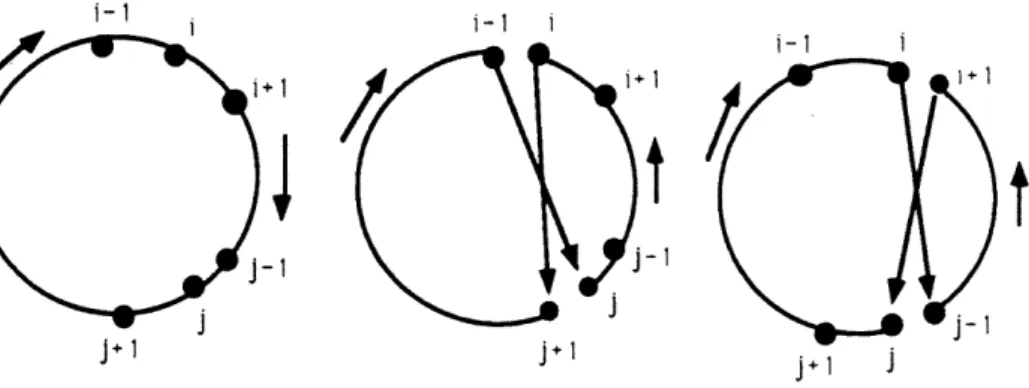
Figure 1: Illustration of the two-interchange procedure. At top is original configuration. In cen-ter is the configuration I(i,j) obtained by incen-terchanging i and j. At bottom is the configuration
I(i + 1,j - 1) obtained by interchanging i + 1 and j - 1.
of Bertsimas and Howell [6] in demonstrating the procedure for the case of the homogeneous PTSP; some details for the more complicated heterogeneous case are given in the next section.
Suppose we have an ordering of points
(1,...,i- 1, i,i + 1,...,j- 1,j,j + ,...,n). Inversion of points i and j gives the new order I(i, j):
(1,...,i- 1,j,j- 1,...,i + 1,i,j + 1,...,n).
The heuristic operates by computing the difference in cost between two configurations obtained from one another via such interchanges. We compute here the cost difference between the configurations
I(i,j) and I(i+ 1,j-1). Let C(i,j) represent the cost of I(i,j). We shall call nodes i+1, ... , j -1 the inside nodes and all others for this configuration the outside nodes (refer to Figure 1). The differences
between one configuration and another are a function of "interactions" between the nodes i, j and the sets of inside and outside nodes. Defining the arrays A and B according to
n-l
Ai,k = Z(1-p)"-ld(i,i+ r)
r=k
n-1
Bi,k =
Z(1-p)r-ld(i,
i-r),
r=k
we have the formula
C(i,j) = C(i + 1,j -1) +
i- i-i i
d
p2 [(q-k _ 1)Ai,k+l + (qk -_ 1)(Bi,1- Bi,n-k)
(qk - 1)(Aj,l - Aj,.-k) + (q-k _ 1)Bj,L+1 +
(q'-k _ 1)(Ai,1 - Ai,k) + (qk-f - 1)Bi,n-k+l +
(qk-n - 1)Aji,n-k+ + (q-k - 1)(Bj,1 - Bj,k+l)] , (14)
where k = j - i, q = 1 - p, and all indices are taken modulo n. Each line of this formula represents a different group of interactions. For example, the first term concerns the interaction between node
i and the set of outside nodes; it may be derived as follows. For the configuration I(i,j), the
contribution to the total expected cost is
n-1 n-k-1
[p2 E d(i, i + r)(1-p)r t + E d(i, i-r)(1-p)r 1 (15)
r=k+l r=1
The term p2 appears because nodes i and i + r (or i - r) must be present, while the requirement that the other nodes be absent gives the apppriate 1-p term. The corresponding expression for the configuration I(i + 1,j - 1) is
n-1 n-k-1
p2 d(i, i + r)(1-p)- '+ d(i,i-r)(1-p) + k . (16)
=rk+l r=l
Subtraction of this expression from (15) gives
n-1 n-k-1
p2 d(i + r)(1- p)rl(q-k _ 1)+ d(i, - r)(1 - p)r-l(qk 1)
r=k+l r=1
which, upon substitution of our A and B notation, becomes the first line of the formula in (14). In a similar fashion to the above, we can obtain the second line of the formula from the interaction between i and the inside nodes, and the third and fourth lines from the corresponding interactions for node j. There are no contributions from other interactions due to the symmetry of the problem (i.e. the fact that all probabilities are equal).
Our implementation of this algorithm consists of two phases. The first of these constructs the arrays A and B and makes a first pass to consider all 2-interchanges of adjacent nodes i, i+ 1, making improvements in the tour without updating the matrices. If an improvement is found, phase one is repeated; otherwise, a second phase is initiated to check for other possible improvements until one is found (upon which phase 1 is re-started). Thus most of the improvement is made in phase one, and the algorithm runs in O(n2) on average.
2.4
The 2-interchange: Heterogeneous PTSP
Our testing procedures also include the 2-interchange heuristic in the case of non-homogeneous probabilities. Here the formula is somewhat more complicated and computationally expensive. For ease of illustration, we present the formula only for the special case where the interchanged nodes are adjacent.
Consider an initial configuration and a final configuration differing only by the inversion of nodes
i and i + 1. Denoting by A(i, i + 1) the difference in cost of the two tours, we have
on-l i+r-1
A(i,i+ 1) = PiPi+l
d(i,i+
r)pi+,J
(1 -Pq)-r=2 q=i+2 n-2 i+r EZd(i+li+ l + r)pi++l (1-pq)+ r=1 q=i+2 n-2 i-r+l E d(i, r)pi- r I (1-P,-r=l q=i-n-1 i-1 Ed(i + 1,i+1-r)pi_,+l H (1-pq) (17) r=2 q=i-r+2
For the more general situation where the nodes are not adjacent, it is a straightforward but tedious matter to generalize the homogeneous case. However, due to the absence of symmetry, there are more interactions between inside and outside nodes. We illustrate this idea briefly.
Referring to Figure 1, we define a clockwise orientation to be movement along the circle clockwise relative to the outside nodes (i.e. in the direction from j + 1 to i - 1 in the top picture), and we define a corresponding counterclockwise orientation to be the opposite. Now we merely note that from the point of view of the node i relative to the outside nodes, the only important difference is as follows: moving in a clockwise fashion from i in I(i + 1, j - 1), the nodes j - 1,..., i + 1, j intervene between node i and the outside nodes, while in I(i,j) the intervening nodes are j,j - 1,..., i + 1, and the direction is counter-clockwise. Thus in I(i, j), the contribution to expected cost from the interaction is
n-1
P, E d(i,i + r)pi+r (1 - p) +
r-=k+l q=j+l
n-k-1 i-i
P[(1 - Pi+l)' (1-pj)] E d(i, i-r)pir H (1-Pq) (18)
while in I(i + 1, j - 1) it is
n-1 i+r-i
Pi[(l-pi+l) (1-pj)] d(i, i + r)pi+r I (1-pq) +
r=k+l q=j+l
n-k-1 i-1
Pi a d(i, i-r)pi-r
II
(1-pq). (19)r=l q=i-r+l
Subtracting (19) from (18), we obtain the net effect of the interchange with respect to this interaction. The other parts of the formula are obtained in similar fashion.
2.5
The 1-shift heuristic: Homogeneous PTSP
In the realm of the TSP there has been some success with the so-called 3-interchange heuristic, which could conceivably be adapted for the case of the PTSP. The idea is to improve an existing tour by shifting an entire section (i.e. a set of nodes lying between two points) to a different location within the tour. An initial ordering of
(1,..,i- 1,i,...,j,j + 1,...,k,k + ,...,n)
becomes, after an insertion of the points i,..., j between k and k + 1, (1,...,i- 1,j+ 1,...,k,i,...,j,k + 1,...,n).
Unfortunately, the additional computational burden created by the probabilistic elements of the objective function make the 3-interchange heuristic unattractive for the PTSP. However, Bertsimas and Howell [6] have introduced the 1-shift, which is a degenerate (and much simpler) version of the general 3-interchange procedure. This we now proceed to describe.
The 1-shift heuristic is obtained above when the set of points i,...,
j
consists only of a single point i (hence the name 1-shift). The procedure differs fundamentally from the 2-interchange in that there is no inversion of points on the tour. Bertsimas and Howell have argued that for small values of p this structure-preserving property makes the 1-shift procedure more efficient. Their argument is as follows. In the case of low p, any reasonable tour (e.g. one obtained via radial sorting) is likely to be a good one already. Thus most inversions are likely to worsen rather than improve the objective function. The 1-shift does not even consider such inversions and therefore saves computation time.To derive the formula for the change in the objective value due to a 1-shift (see Figure 2), consider an initial configuration
(1,...,i-,ii + ,...,j- 1,j,j +
1,...,n)
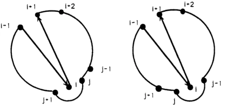
i-i i+2 i+1 i+2 i j-i j- - 1
Figure 2: Demonstration of the 1-shift procedure. At top is the configuration S(ij); below is the configuration S(i,j - 1). The arrows indicate the original tour.
which becomes after a 1-shift of node of node i after j
(1,...,i- 1, i+ ,...,j- 1,j,i, + 1,...,n).
Denote the latter configuration by S(i, j) and its cost by C(i, j). Then we have the formula (for details see [9])
C(i, j) = C(i,j - 1) +
p2 [(q-k q-(-))Ai,k+ 1 + (qk - qk-l)(Bi l- Bin-)+
(q - 1)(A/1 - Aj,n.-k) + (q-' _ 1)Bj,k+l +
(q,-1-k - qn-k)(Ail - Ai,k) + (qk-n - qk-(n-l))Bi,,,k+l +
(1 - q-1)Aj,.k+l + (1 - q)(Bj,1 - Bj,k+1)l , (20)
taking all indices modulo n.
As with the 2-interchange, the symmetry of the homogeneous problem simplifies the calculations.
2.6
The 1-shift: Heterogeneous PTSP
The 1-shift formula (20) can be extended to the heterogeneous case in the same manner as the 2-interchange procedure. We omit the straightforward but tedious derivation.
2.7 Sampling and Re-optimization
As mentioned at the outset, the goal of our investigation was to compare a priori heuristics with strategies of re-optimization. Of course in practice exact re-optimization procedures are often not computationally feasible. In our case, where the intent was to develop algorithms capable of being run on small computers, exact methods proved impossible for problems of any reasonable size. The set of possible outcomes to the PTSP has cardinality 2, so that even a fast machine would confront a huge number of problems to be solved in order to obtain an expected cost. Thus in our studies we were led to consider pseudo-reoptimization, employing (deterministic) heuristic procedures and a sampling technique which we now describe.
Let us denote by Si a sample of points (generated from the n total points) representing locations having a demand on a given realization i, i = 1,..., N where N is the number of samples taken. Supposing for the moment that exact optimization were possible for each corresponding TSP, the law of large numbers suggests that for large enough N,
E[PTSP] , $'--1 p(Sj)LTSP(Si) (21)
N
suggesting a lower bound for our a priori solution. The variance of the estimate so obtained can be reduced through the use of a control variate procedure. To see this we write
E[ETSP] = E p(S)(LTSP(S) - L(S)) + p(S)L(S) (22)
SCv sCV
The last term of this equation, which we shall denote as ', can be computed exactly once the heuristic tour has been found. The first term, which we call t - t', must be computed using Monte Carlo sampling. If we let s2denote the sample variance for the estimate of E[ETSP], we have that
s2 = Var(t - t' + 0') = Var(t) + Var(t') - 2Cov(t, t'). (23) Since we expect that the terms t and t' will be strongly positively correlated, the technique should (and does) improve our estimate's variance.
Before computational testing could begin, we confronted the question of what method to use in solving the sampled TSP's. Since our test problems were on graphs of 100 nodes and our algorithms intended for use on personal computers, heuristic procedures were necessary; nevertheless we wished to achieve close to optimal results for purposes of comparison. A reasonable compromise between tractability and accuracy was achieved by taking for each problem the minimum of two tours, one obtained via SFC plus 3-interchange, the other obtained as the minimum cost tour of IS1/5 randomly generated permutations of the (randomly generated) set S.
3
Computational Results for the
PTSP-In this section we briefly present some of the implementation details and then present and analyze our computational findings.
3.1
Implementation Details
We implemented the heuristic and sampling algorithms in a package written for the Apple Macintosh. This package also contains algorithms for the TSP, k-TSP, k-PTSP, VRP, and PVRP. For this
application we used the C programming language and also made extensive use of the graphics capabilities of the Macintosh Toolbox (for menus, graphics, etc.) We present here only some of the
more important details.
We begin with the user inputs. Principally, these are the number of points n for which the PTSP is to be solved, the common probability p (in the case of a homogenous problem), and the type of heuristic (SFC or radial sort) to be used in constructing initial TSP solutions. If heterogeneous probabilities are specified instead, these are generated randomly on the interval [0, 1] and stored as a vector of length n. The locations of the points (cities) are specified as n-vectors of z- and y-coordinates, either directly by the user, or as randomly located in the unit square. Distances are stored in a matrix, though space considerations in larger problems may warrant more sophisticated methods. All tours constructed and modified in the course of a solution are maintained in the following way. At any given time, the current tour is stored as a permutation of the integers 1,...,n. This permutation acts as an index for the coordinate vectors. Thus z[tour[i]] gives the z-coordinate of the ith point on the current tour.
After the input of the initial parameters, the program calculates and displays an initial TSP tour through all points, using the heuristic specified earlier. With this initial tour as a basis, the user is then free to try either of the local improvement techniques to modify the tour. As the tour is improved, the display on the screen shows the changes and the percentage improvement in the objective function. There is also a batch option available to specify a series of problems (e.g. random problems) to be solved. The sampling/re-optimization scheme is also run under this option.
3.2
The Testing Procedure
Our testing procedure was as follows. In the homogeneous case, we generated five problems (n = 100) for each of the common probabilities p = 0.1,..., 0.9. By a problem we mean a set of n random
locations in the unit square. Each problem was then solved by each of the four combinations of heuristics (space-filling curve plus interchange, space-filling curve plus 1-shift, radial sort plus 2-interchange, and radial sort plus 1-shift) in addition to the re-optimization scheme. In the latter case, for each problem, 50 instances (i.e. sets of nodes S) were generated and the corresponding TSP solved to near-optimality. The five problems were different for different probabilities (i.e. there were 45 separate problem-probability combinations), but in a separate testing procedure, the same five problems were used across all values of p, in order to see the effect of p on solution values.
In the case of the heterogeneous PTSP, we generated five original problems. For each of these we generated n random probabilities P,..., p, and solved with the same four combinations of heuristics.
For the re-optimization, 50 instances of the TSP were sampled for each problem, with each point i appearing in the corresponding TSP according to its probability pi. We turn now to a consideration of the results.
3.3 Conclusions
The homogeneous PTSP
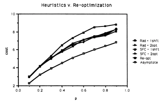
Tables 1 and 2, together with Figure 3, summarize the chief computational test results for the heuristics we have described. We have not included running time here but choose instead to make some qualitative remarks in this regard. The data consist of 5-problem averages of the objective value attained by four diffferent heuristics and re-optimization. Table 1 refers to the homogeneous case, with the common probability ranging from 0.1 up to 0.9. As is evident from the figure, all heuristics, with the sole exception of radial sort + 1-shift, give roughly the same performance. Moreover, they are also close in performance to the re-optimization heuristic, typically within 1%. Since we suspect that the latter gives results which are quite close to optimal, the data suggest that the a priori tours constructed have low expected cost, an observation which has considerable practical significance. As noted at the outset, the a priori approach demands far fewer resources than re-optimization and establishes a uniformity of service which re-optimization cannot provide. All of this makes a priori solutions far more easy to implement, so the additional fact that computational experiments suggest good cost performance is an encouraging fact.
The worst performing heuristic appears to be radial sort + 1-shift. Re-optimization costs are usually better than those for the a priori heuristics, but the differences are not great. However, radial sort + 1-shift gives consistently higher cost, ranging all the way up to a 14% difference at the higher values of p. The explanation for this relatively poor performance probably has more to do with the
P Objective Value (avg. of 5)
Rad + lshft Rad + 2opt SFC + lshft SFC + 2opt Re-opt.
0.1 2.9848 2.9806 2.9921 2.9909 2.9844 0.2 4.1539 4.1173 4.1813 4.1847 4.1262 0.3 5.2879 5.0383 5.0644 5.0311 5.1035 0.4 6.4961 5.8413 5.9410 5.8886 5.7742 0.5 7.2901 6.6037 6.7231 6.5663 6.3741 0.6 7.8895 6.8543 7.1218 6.8726 7.1032 0.7 8.5207 7.4124 7.5276 7.4433 7.4028 0.8 8.6378 7.8531 7.7075 7.6216 7.5826 0.9 8.8538 8.2652 8.3171 8.3499 8.0551
Table 1: Heuristics vs Re-optimization: Homogeneous PTSP
Heuristics v. Re-optimizatlon .0 0.2 0.4 0.6 0.8 -I Rad + Ishft - Rad + 2opt -I SFC + Ishft -e SFC 2opt _ Re-opt 4 Asymptote I .0 p
Figure 3: Heuristics vs. Re-optimization for the Homogeneous PTSP
10- 8-0 6-o 2-0 U - I - I~~~~~~~~~~~~~~~~ r r r I
1-shift procedure than with radial sort. As noted earlier, the radial sort has good properties for low values of p, where the coupling effects of node-interactions become relatively more important. This idea is confirmed by the table entries for p = 0.1,0.2. At higher values of p, however, the importance of the coupling effect diminishes, and in general the radial sort is inferior to SFC. More important than this, however, are the characteristics of the 1-shift procedure. The 1-shift procedure tends to preserve original order, while 2-interchange attempts to make numerous inversions. Our intuition is that in considering these inversions, 2-interchange examines a wider range of potential improvements, despite the fact that the 1-shift procedure actually operates over a larger space. By considering more radical alterations in the shape of the design, 2-interchange succeeds in achieving a lower cost overall.
We believe that the choice of radial sort versus space-filling curve is of relatively little consequence
as long as the subsequent improvements considered (via local optimization) are extensive enough. In
the case of 1-shift, the difficulty arises because the original shape is not exposed to a wide enough series of possible transformations.
With regard to running time, all heuristics for the homogenous PTSP were quite fast, with the 2-opt procedures considerably faster (by a factor 2 or 3) than their 1-shift counterparts. The algorithms were easily implemented on small personal computers - in our case, the running time for a single 2-opt problem of 100 nodes (with p = 0.7, say) was on the order of 2-3 minutes (increasing, of course, in the value of p) on a Macintosh II. To run the entire set of 45 problems (with p ranging from 0.1 to 0.9) took about 1 1/2 hours at the shortest (SFC + 2opt) and 4 hours at the longest (radial sort + 1-shift). Taken together with the cost data of the table, this information suggests that in the homogeneous case, a combination of the spacefilling curve and 2-interchange heuristics quickly produces tours which have close to optimal expected cost. From a practical standpoint, this combination gives the best performance.
Also included in the figure is a curve indicating the asymptotic expected cost of the PTSP, which for large n is
Cn ~ 3TSPV,
where PTSP T 0.72. We see that for n = 100, asymptotic cost is not yet achieved, although the actual cost does follow roughly the same trajectory as the asymptotic cost over the range of p.
The heterogeneous PTSP
The heterogeneous case differs in several respects from the homogeneous one. Computation times for the heterogeneous case were significantly higher than for the homogeneous case, with all a
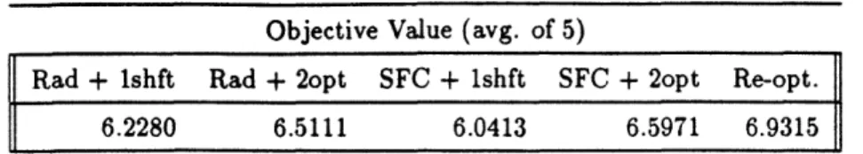
Objective Value (avg. of 5)
Rad + shft Rad + 2opt SFC + lshft SFC + 2opt Re-opt.
6.2280 6.5111 6.0413 6.5971 6.9315
Table 2: Heuristics vs Re-optimization: Heterogeneous PTSP
priori heuristics requiring over twelve hours to finish (5 problems). In fact, in the case of the
2-opt procedures, run-times were so excessive that we chose instead to impose a truncation scheme on the number of allowable iterations (hence the higher costs for the combinations employing 2-opt). The reasons why 2-opt is slow for heterogeneous demands while it is fast for homogeneous demands are clear: the computational burden of computing the expected costs (which must be evaluated to compare local alternatives) is substantially higher in the heterogeneous case. The practical implications of the loss in speed are not too severe, however, since the truncated algorithms (which run very quickly - five problems in 23 minutes) give reasonably good answers.
A noticeable phenomenon in the heterogeneous case is the superiority of all a priori procedures over heuristic re-optimization, by a margin of about 8% in the case of the 1-shift procedures. This finding is in contrast to the homogeneous case, where the heuristic re-optimization procedures dif-fered only slightly from the others. There is some explanation for this finding. The heuristics used in the re-optimization tend to perform well when the demand points are uniformly distributed, but their performance deteriorates when there is significant clustering. While homogeneous probabili-ties tend to give a uniform distribution of points with positive demand, in the heterogeneous case, clustering is more likely. Moreover, the non-reoptimization heuristics are fairly sophisticated in that they take careful account of the interactions between nodes (i.e. they explicitly consider the effect that each node's presence or absence has on the others in the tour).
While the heterogeneous case is certainly more difficult, our conclusion is that the truncated versions of the heuristics perform well, both in terms of run time and objective value. With their attractive simplicity, they should prove useful in practice.
4
Heuristics for the 1-Vehicle Stochastic Routing Problem
From the PTSP we now turn to the 1-vehicle PVRP, for which we propose a heuristic we call the cyclic heuristic. After presenting some worst-case analysis for this heuristic, we introduce some refinements (local improvement procedures and dynamic programming) and perform computational experiments.
4.1
The Cyclic Heuristic
The cyclic heuristic develops a visitation strategy for the 1-vehicle PVRP based on a TSP tour of the
n demand points. By visitation strategy we mean an a priori plan for visiting the demand points.
Given any route on the n demand points, a visitation strategy is obtained by starting at the depot and visiting points as specified by the route, returning to the depot whenever capacity is reached. Under strategy a, all points are visited, whereas for strategy b, wherever a zero demand is realized, it is skipped. Most of our analysis restricts attention to strategy a; some remarks at the end of the section address strategy b.
A simple example illustrates the idea of a visitation strategy. Suppose the TSP solution is 2, 4, 3, 1 and the vehicle reaches its capacity in the course of fulfilling demand at point 3. In this case, it returns to the depot, empties its load, and resumes its tour at point 3. If the remaining demand at 3 plus the demand at 4 does not exceed capacity, the final route is 0-2-4-3-0-3-1-0.
Note that by considering each of the n points of the tour as a starting point (i.e. the first point to visit after leaving the depot), we obtain n potential visitation strategies. The cyclic heuristic works by considering each of these n possibilities and selecting the one with the best expected cost, which is given by the expression
~~n
nE[Lr] = (1 -i)d(id i + 1) + (2d(i, 0) + i[d(i, 0) + d(i + 1, 0)]), (24)
i=O i=1
assuming that the underlying tour is 1, ... , n. This formula is merely that of equation (10) re-written by expanding the terms s(i, i + 1).
Prior to computational testing, we assess the worst-case performance of the cyclic heuristic and examine its asymptotic behavior relative to a strategy of re-optimization. The following are the two major results, which hold under the so-called visitation restriction, the requirement that under re-optimization, all locations must still be visited (as in strategy a). We employ the terminology
L, _ (random) cost of cyclic heuristic solution under strategy a III
Ra = (random) cost of re-optimization solution under strategy a n
-
Zd(O,
i)/ni=l1
3 SP
= BHH constant for Euclidean TSP - 0.72.
Theorem 1 For strategy a under the visitation restriction,
E[L] < 2. (25)
Theorem 2 Let X1, ... , Xn be a vector of i.i. d. demands, whose locations (together with the location
of the depot) are independently and uniformly distributed throughout the unit square. Then for a vehicle with capacity Qn under strategy a,
(i)If hi; - 0 as n -, oo then
lim QnE[LI ] = 2E(X)? (26)
n-oo n
(ii)If Qn - oo as n - oo then
lim E[L]= /TSP (27)
n-oo /
Similarly, for strategy b with p = Pr{zero demand},
(iii)If - -- O as n - oo then
lim QnE[L] = 2E(X)r (28)
n-oo n
(iv)If Qn - oo as n - oo then
lim E[a = d(p) (29)
n-floo/-where *Tspv/ < ,3(p) < 0.92V/.
For proofs of the above theorems see Bertsimas [7].
Note that under strategy a, the above shows that the cyclic heuristic is asymptotically optimal if the initial tour is the optimal TST. The heuristic is also asymptotically optimal for strategy b in the case where limnO 0. = 0.
In practice, of course, the optimal TST is not available; instead, we must begin with a heuristic solution. However, there are several practical refinements which can be made to the cyclic heuristic. We describe these next.
4.2
Local Improvement Procedures
In the case where the node demands are independent and identically distributed (what we have called the homogeneous PVRP), the initial TSP tour can be refined via local improvement procedures. These rely on the fact that with a homogeneous PVRP, the return probabilities 7i and i depend only on the order (and not the identity) of the nodes. Although the procedure to be described here could be adapted for strategy b, the details are quite tedious and the computation expensive. Therefore, as we noted above, we consider only the case of strategy a here.
The local improvement algorithm is a 2-interchange procedure similar to those used for the PTSP in the previous section. It uses the expected cost (24) as the objective value, considering at each step the potential improvement which would be obtained upon inverting a section of the tour between a current pair of nodes. For example, if the pair is (i,j), an initial ordering of
(1,...,i-,i,i+ ,...,j-l,j,j+l,...,n)
would become
(1,...,i- 1,j,j- 1,...,i + 1, i,j + 1,...,n).
Again we shall distinguish between outside and inside nodes. In light of the previous remarks for the homogeneous PVRP, the contribution of the outside nodes 1,. .. , i - 1 and j + 1, ... , n in (24) is unchanged. For the inside nodes, there is a change 6 = - i, where
i j j-1
6,b= (1- y)d(k,k + 1)+ (26 + )d(k,0)+ i - d( + 1,0)
k=i-1 k=i k=i-1
b! = (1- 7i- 1)d(i - 1,j) + (1 - yj)d(i,j + 1) + Z(2i+j k d(k, 0)) +
k=i
j-1 j-1
Z(1-
7i+j-kl)d(k,k + 1)+ E ?1i+j-k-2d(k + 1,0).k=i k=i-1
The derivation of these expressions is straightforward bookkeeping, given the definitions of the break probabilities 6 and y. Local improvement proceeds by making all interchanges where 6 > 0.
Local improvement may be incorporated into the cyclic heuristic in two ways. Most simply, it may be used to improve the initial TSP tour, resulting in a new initial tour for the cyclic heuristic. Alternatively, local improvement may be attempted for each cyclic permutation of the original tour (this obviously is more expensive computationally). The test results to follow shortly reflect this second, more expensive implementation. In either case, subsequent improvement in the cost function is possible via the dynamic programming procedures introduced next.
4.3
Dynamic Programming Procedures
All procedures described thus far are static in the sense that information obtained en route (i.e. by the driver) does not affect decisions. Incorporating such information simply is the essence of the dynamic programming procedure described next. Suppose then that we have an initial tour, say a good TSP tour, on the demand points. We can then describe a dynamic programming problem in which the decision points occur each time the vehicle departs a demand node i carrying a given load k. We define C(i, k) to be the expected remaining distance to travel, given that the optimal strategy is followed, when the vehicle has just visited node i - 1 and is now carrying a load k. At each decision point, the choice is either to continue to the next point i (and risk the possibility that the additional demand there will exceed the remaining capacity Q - k), or to return to the depot to drop off the current load before proceeding to node i. Because the triangle inequality is assumed to hold throughout, it will sometimes be better for the vehicle to return to the depot only partially full, since there may be substantial probability that otherwise the vehicle will become full before filling all of the demand at the next location (necessitating a return trip to the depot and a second trip out to fill the remaining demand). Such a cautious strategy will especially pay off in the case where the next location is quite distant from the depot and thus quite expensive to visit more than once.
We may formally write the dynamic program as follows. Define the maximum demand value for node i to be K(i)[K(i) < Q Vi]. Then noting that PI = 0 for j > K(i), we have
Initialization:
C(n +1,) = d(0,n)
Recursion (for i = n,. .. , 2):
Q
C(i,k) = min d(, i - 1) + d(O,i) + E C(i + 1,j)p,
j=o
Q-k
d(i- 1,i)+ E C(i + 1,k + j)pi + j=o Q ' Z2> p p(2d(0, i)+ C(i + 1, + j - Q)) j=Q-k+l and k*(i-1) =
min k C(i, k) = d(O, i- 1) + d(O, i) +
Z
C(i+ 1,j)pi .I
inj= 1~~~~j=1The first three terms within the curly brackets reflect the strategy of returning to the depot first. This cost consists of the distance from the present point to the depot (d(O, i)), the distance from the depot to the next point on the tour (d(O, i + 1)), and the expected remaining cost entailed in proceeding with the tour from that point. The second group of three terms reflects the strategy of continuing to the next demand point. This cost consists of the direct distance-cost of proceeding to the next point, (d(i - 1, i)), plus the expected remaining cost entailed in continuing from there. This in turn is divided into two summations, reflecting the two possibilities of exceeding or not exceeding capacity at the next point. The former possibility incurs a cost of 2(d(0, i)) of a return to the depot necessitated by its full load. The term k*(i) is what we have called the threshold value for node i and has a very straightforward interpretation: if the load after visiting node i is at least k'(i), it is optimal to return to the depot before filling further demands. These threshold values, together with the underlying order of visitation, constitute a solution for any given starting point, and the expected total cost is simply =_o pC(2,j) + d(O, 1).
Note that the dynamic program runs in O(nK2) time and requires O(nK) storage capability,
where K = max{K(i)}. Unlike the local interchange argument described above, the dynamic programming procedure does not require that demands be identically distributed.
4.4
The Full Cyclic Heuristic
There is an important difference in philosophy between local improvement and the dynamic pro-gramming approach: the former assumes that the vehicle only returns to the depot when full, while the latter allows the vehicle to return partially full. It is not clear on theoretical grounds whether together the two procedures will always produce a better solution than that which would be obtained by dynamic programming alone (starting with just an initial TSP tour). On the other hand, the dynamic program can only improve upon a local optimization solution. An important question is whether the local improvement substantially improves cost, since its inclusion increases run time.
Assuming for the moment that we include local optimization at each of the n steps, we have the full cyclic heuristic as follows:
Algorithm for strategy a:
1. For demand points 1... n compute a solution to the TSP using a set of good heuristic proce-dures.
2. For each of the n orderings implied by the cyclic permutations of the above tour, use local optimization to obtain a new tour. Then apply the dynamic program to both the original tour
and the improved tour, obtaining threshold values in each case. 3. Choose the lowest cost visitation strategy of these 2n possibilities. 4. Output the final tour, its expected length, and the threshold values.
We remark that the full cyclic heuristic is technically not polynomial time because the local im-provement procedures are exponential in the worst case. A simpler version of the heuristic (omitting local improvement) has complexity O(n2K2).
4.5
Remarks on Case b
Although we have not presented any detailed analysis, the cyclic heuristic may of course be adapted for case b, where zero demands are skipped. Local improvement procedures based upon expected cost are again available, though they are more computationally demanding. The dynamic programming procedure is not adaptable to case b: the computation of the threshold values is only possible a priori because we know that all nodes must be visited. Under strategy b, we obtain prior information that some nodes have zero demand, but incorporating this information into the tour design amounts to pseudo-reoptimization. While our computational testing is solely for the case of strategy a, we suspect that the algorithm will also work well when adapted for case b.
5
Computational Testing for the Cyclic Heuristic
5.1
Implementing the Cyclic Heuristic in 'C'
We describe one implementation of the cyclic heuristic under strategy a. This implementation is the one used for all of the subsequent testing, which was performed on a DEC 3100 Vax work-station computer. As noted earlier, the original PVRP program was part of a larger package for Macintosh; unlike in the case of the PTSP, however, the running times (especially for heterogeneous demands) and memory requirements exceeded the capabilities of small Macintosh machines. How-ever, a significant part of this complexity arose from the need to compare different features (e.g.
local improvement versus dynamic programming). In practical terms, this means that the more streamlined versions of the algorithm (e.g. dynamic programming with no local improvement) are implementable for smaller machines. As mentioned earlier, the complexity of the most streamlined version is O(n2 K 2). In what follows, we present some of the more important implementation details.
The program begins with the input of the necessary parameters: the number of nodes n, the vehicle capacity Q, and the type of demand distribution. The type of distribution, e.g. normal, is assumed to be the same for all demand points, though the parameters, e.g. the means and variances, may vary. Our program handles two types of distributions: a discretized normal distribution and a discrete uniform distribution. In the former case, the user specifies a mean and standard deviation for the demand at each node, and the discrete probabilities are calculated on the basis of a standard normal table with a suitable rounding procedure. For the more simple discrete uniform case, the user merely specifies the range for each node demand.
Given these parameters, the first step in the program is the calculation of the probabilities i and i via the procedure described in section (1). If the demands are specified to be identically distributed, this calculation need only be done once, since in this case, a change in the order of the points merely permutes the values of the yi's and 6i's. In the case of non-identical demands, local improvement is not used, and the only reason for calculating the probabilities is the calculation of the expected cost without dynamic programming (the dynamic programming procedure calculates its own expected cost as part of the recursion - hence our remarks above on streamlining the procedure by omitting local optimization).
The main part of the program proceeds as follows. For each of a (user-specified) number of problems, the user may specify the locations of n points in the unit square, or these points may be taken to be independently uniformly distributed. As with the PTSP, x- and y- coordinates for points 1,..., n are stored as n-vectors, and inter-node distances are computed and stored as a matrix. An initial TSP solution is constructed via SFC and improved via a combination of 2- and 3-interchange procedures. The traveling salesman tour so obtained is usually with 2-3% of optimal. The principal inner loop of the program consists of permuting this initial tour by one place each time. For each permutation, local-optimization is performed (if specified so by the user), and the dynamic program is run to calculate the threshold values. For the dynamic programming, we use a cost matrix C, where C[tour[i]][k] denotes the expected cost remaining after departing the i - th node on the tour carrying a load of k. The algorithm works backward from the nth node in the usual fashion. Thus at each of the n iterations, we calculate both an expected cost without dynamic
programming (c.f. eq.(24)) and an expected cost incorporating the threshold values. The best cost value is updated over the course of the loop, and the corresponding tour saved. The output consists of the two tours obtained plus the threshold values for the second tour. For the Macintosh version, graphic displays are available.
5.2 Strategies of Re-optimization
As in the case of the PTSP testing procedures, the ideal candidate for comparison is a strategy of re-optimization in which the (optimal) exact routes are formulated once the demands are known. To obtain a full comparison, one would generate all instances of demand for the given demand distribution(s), solve each instance optimally, and calculate an overall expected cost
E[L']= E P(il .... in)L'(il,..., i.), (30)
il ,.,iu,
where L(il,..., i,) is the optimal vehicle routing cost for the demand realization (X1 = il,..., X, = in) and P(-) denotes the (discrete) joint demand distribution on n nodes.
Even more so than in the PTSP case, there are prohibitive computational problems with such an approach. The number of terms in the summation in (30) is enormous for all but very small problems (for example, if the demands are independently discrete uniform on [1, 10], the total number of VRP's to solve is 10n). To overcome this problem of dimensionality, we again employ sampling ideas. Instead of considering all instances of demand, we generate a sample of the demands from the underlying distribution and solve these instances optimally. Each sample yields solution with cost L*(i,... ,i), with k indexing demand samples and ranging from 1 up to S. An estimate of the overall expected cost in following a re-optimization strategy is then
S
Lr T/~ k1(31)
S = S
E
L
,.).,in)
(31)
k=1
While this approach eliminates the problem of the large state space, the estimation implicit in (31) is still quite computationally intensive because of the requirement that each sample VRP be solved to optimality. For small n, exact solutions to the VRP can be obtained easily, but problems bigger than 15 nodes quickly become intractable. For example, a dynamic programming formulation of the problem in [10], in the absence of additional side constraints, essentially amounts to a complete enumeration of all subsets of nodes (examining each subset as a potential subtour), an enumeration of 2" sets. Thus, in order to conduct tests on problems of reasonable size, we are forced to abandon true "re-optimization" as the standard for comparison.
With exact optimization possessing these drawbacks, it is sensible to consider instead good heuristic solutions. Following this idea, for each sampled demand instance we solve the corresponding VRP by a (deterministic) heuristic to obtain a cost Lh(il,...,in). For S samples we obtain the estimate
=~ E h(ik, ik(32) k=l
This is the approach we have employed in our testing.
We implemented two heuristics for the VRP: a clustering heuristic due to Christofides, Mingozzi, and Toth [10] and the well-known Clarke-Wright savings algorithm [11]. The clustering heuristic groups nodes into clusters according to a local cost criterion, then constructs subtours through these clusters using heuristic TSP procedures. Particular nodes are chosen as initial seed points, and the remaining nodes are assigned according to this measure of relative cost, thereby forming a cluster. The local cost criterion may be simple distance to the seed, average distance to all points in the existing cluster, or some other suitable measure. Clusters are formed both sequentially and in parallel, with the better solution selected. The program requires a somewhat extensive use of data structures. The Clarke-Wright procedure begins with each demand point on a separate subtour, then consolidates these separate tours according to the potential savings realized by such consolidation.
Both algorithms were encoded on the assumption that all points (including zero-demand points) were to be visited, in keeping with our testing of strategy a.
5.3
The Testing Procedure
Although our code was originally intended for the MacIntosh (to take advantage of the graphics package available there), for the purposes of testing we uploaded onto a VAX 3100 Workstation using the more standard version of C. This change was necessary in order to obtain results for larger problems (greater than 20 nodes) in a reasonable amount of time. However, as noted before, simpler versions of the algorithm (i.e. those not performing local optimization and not calculating the return probabilities) have shorter run-times.
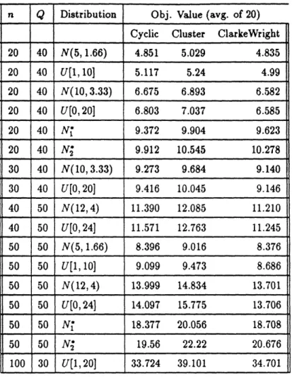
The testing format was as follows. For each type of PVRP (a type corresponding to particular values for n, Q, and the demand distribution), 20 test problems were constructed by randomly choosing n points in the unit square. In the case of the re-optimization heuristics, for each of these test problems 100 demand instances were simulated according to the specified distributions. We obtained estimated re-optimization objective values by averaging over instances for each problem,
n Q Distribution Obj. Value (avg. of 20) Cyclic Cluster ClarkeWright
20 40 N(5,1.66) 4.851 5.029 4.835 20 40 U[1, 10] 5.117 5.24 4.99 20 40 N(10, 3.33) 6.675 6.893 6.582 20 40 U[0, 20] 6.803 7.037 6.585 20 40 N' 9.372 9.904 9.623 20 40 N 9.912 10.545 10.278 30 40 N(10, 3.33) 9.273 9.684 9.140 30 40 U[0, 20] 9.416 10.045 9.146 40 50 N(12,4) 11.390 12.085 11.210 40 50 U[0, 24] 11.571 12.763 11.245 50 50 N(5,1.66) 8.396 9.016 8.376 50 50 U[1,10] 9.099 9.473 8.686 50 50 N(12,4) 13.999 14.834 13.701 50 50 U[0, 24] 14.097 15.775 13.706 50 50 N' 18.377 20.056 18.708 50 50 N* 19.56 22.22 20.676 100 30 U[1,20] 33.724 39.101 34.701
Table 3: Cyclic Heuristic vs. Re-optimization
and we then obtained for
obtained expected
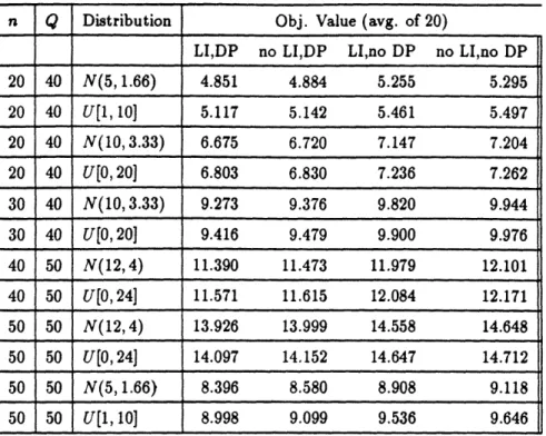
an overall average for the 20 problems. For the cyclic heuristic, values were costs under four scenarios: no dynamic program and no local optimization (basic heuristic), no dynamic programming with local optimization, dynamic programming without local optimization, and dynamic programming with local optimization.
5.4
Discussion
We turn now to a discussion of our computational results. There are a number of issues to address: * How does the cyclic heuristic compare to re-optimization?
* At what problem size does asymptotic behavior emerge?
* What are the relative effects of local improvement and dynamic programming procedures? * What are the relevant conclusions for the practitioner?
Consider first the comparison of the cyclic heuristic to re-optimization. Our expectation prior to testing was that the cyclic heuristic would perform quite well, considerably better than its worst-case bound of two. Our test results against heuristic re-optimization procedures do suggest that the a priori approach works well. Consider the data of Table 3. Here we have classified problems according to n, Q, and demand distribution. With respect to the latter category, N(p, a) denotes a discretized normal distribution whose continuous version has mean p and standard deviation a, while U[a, b] denotes a discrete uniform distribution on the interval [a, b]. These two distributions correspond to identically distributed demands. We have also included two other distributions, N; and N2, which denote independent but non-identical normal demands at the n nodes (i.e. normal demands of different means and variances). For example, the distributions N; are a repeating cycle of N(10, 3.33), N(16,5.33), N(26,8.66), N(20,6.66), N(14,4,66), N(24,8), N(18,6), N(12,4), and
N(22, 7.33) (the cycle repeats every nine nodes). The distributions N2 are similar but have wider
variation between nodes.
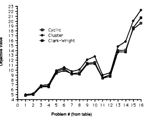
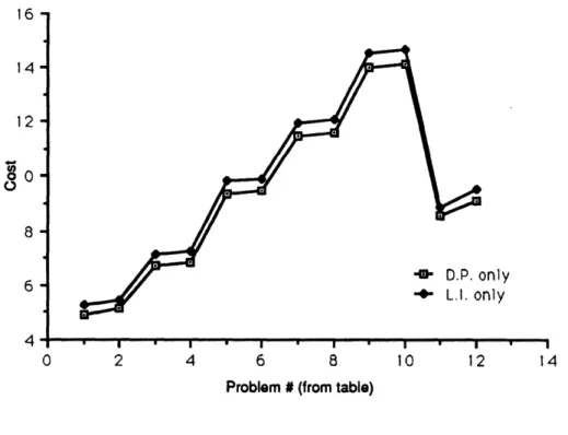
Figure 4 gives a graphical summary of the data in the table, showing the objective values for the three different approaches (Clarke-Wright, cluster heuristic, full cyclic heuristic) for the first 16 test problems of the table. From the data, we see that the cyclic heuristic performs very impressively in
comparison to re-optimization. In fact, the heuristic is consistently superior to the cluster scheme,
giving a lower objective value for all problems considered, the margin of superiority ranging from around 2% for the smaller test problems up to 16% for the 100-node problem. This result agrees with the finding that vehicle routing heuristics based upon cluster first - route second schemes can be asymptotically sub-optimal. This claim has been demonstrated in the case of the well-known sweep heuristic [12], and it seems also to be the case here, although our results do not cover large "asymptotic" cases. But even for the smallest problems we consider, the cyclic heuristic dominates the cluster procedure and does so for a number of choices of the local cost criterion.
Clarke-Wright does manage to out-perform the cyclic heuristic for problems smaller than 50 nodes, but the margin of superiority is never more than 3%. Moreover, in all cases where demands are non-identical, the cyclic heuristic outperforms both of the re-optimization schemes. While we certainly are not surprised to see behavior which departs from worst-case expectations, the results here suggest that Clarke-Wright does not perform well under certain conditions of widely- varying demand, quite probably due to clustering effects. It is also clear that for larger problems, the cyclic
Cyclic heuristic v. re-optimization
-a- Cyclic -- Cluster -- Clark-Wright - ,-u.u-E-s-I,.,-I.I-I-,u-..I. I 0 1 2 3 4 5 6 7 8 9 10 11 12 13 14 15 16Problem # (from table)
Figure 4: The heuristic vs. re-optimization 25' 22' 21 20 19 18 17 16-> 15-_ 14-13 12- 8- 7- 6- 5-A. A--- .I-III-I-I-I-II-III-I-I-I-III-I
Asymptotic Behavior of Cost
r D)/Q ial cost 100 No. of nodes 200Figure 5: Comparing asymptotic and actual objective values
heuristic out-performs both re-optimization schemes. This phenomenon reflects the asymptotic optimality of the cyclic heuristic, a characteristic which is not shared by the others. Our results show that the margin of superiority of Clarke-Wright shrinks as the number of nodes increases, with the cyclic heuristic eventually gaining the edge. For example, in the 100-node test problem, the cyclic heuristic is better by 3%. We also note here briefly that the greater variance of the uniform demand distribution increases cost (relative to a normal distribution with the same mean), a phenomenon which is not surprising.
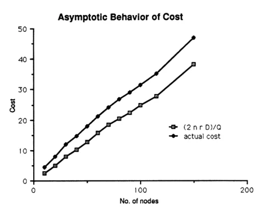
Asymptotic behavior of the heuristic is another matter to consider. Figure 5 illustrates one example. Here we have plotted the objective values obtained for single test problems with different values of n. For all of these problems, Q = 30 and the demand distribution is U[1, 20]. Included also are the values of 2nE[D] / Q, the expression for the asymptotic cost when capacity is held constant. We see here quite clearly the rough linearity of the objective value under these circumstances. The objective value and the asymptotic value differ by a roughly constant amount up to n = 150, the
50 -40 -30 20 - 10-0* 0 I I =