Compression of underwater video sequences with quantizer/position-dependent encoding

(1)

Compression of Underwater Video Sequences with Quantizer/Position-Dependent Encoding

by

Theresa Huang

Submitted to the Department of Electrical Engineering and Computer Science in Partial Fulfillment of the Requirements for the Degree of

Master of Engineering in Electrical Engineering and Computer Science at the Massachusetts Institute of Technology

June 4, 1999

The author hereby grants to M.I.T. permission to reproduce and distribute publicly paper and electronic copies of this thesis

document in whole or in part.

Author

Department of Ela~trical Engineering and Computer Science May 17, 1999 Certified by ~< - Jae S. Lim }Jesisfupervisor Accepted by Xrthur C. Smith Chairman, Department Committee on Graduate Theses

MASSACHUSETTS INST OF TECHNQ

(2)

Compression of Underwater Video Sequences with Quantizer/Position-Dependent Encoding

by

Theresa Huang Submitted to the

Department of Electrical Engineering and Computer Science May 17, 1999

In Partial Fulfillment of the Requirements for the Degree of Master of Engineering in Electrical Engineering and Computer Science

Abstract

Transmission of an underwater video sequence obtained from an unmanned underwater vehicle at

10 kilobits per second (kbps) requires that the data to be compressed by a factor of over a

thou-sand. In order to obtain such low bit-rates, the video sequence is first preprocessed. Motion esti-mation is used to reduce the temporal redundancies, and the Discrete Cosine Transform (DCT) is applied to 8x8 blocks to minimize the spatial redundancies. Each 8x8 block of DCT coefficients is then quantized and encoded into a bit stream. Typical compression standards use two code-books to assign a codeword to each event that occurs. Quantizer/Position-Dependent Encoding

(QPDE) achieves greater compression by designing a separate codebook for each starting position

and quantizer. QPDE exploits the fact that the statistics of the events vary as a function of the starting position and the quantizer. As a result, QPDE successfully reduces the bit-rate to 10 kbps without compromising the quality of the underwater video sequence.

Thesis Supervisor: Jae S. Lim

(3)

Acknowledgments

I would like to thank my thesis supervisor, Professor Jae S. Lim and Eric C. Reed for their

guidance and advice during this project. I would also like to thank all the other graduate student and Cindy LeBlanc at the Advanced Television Research Program (ATRP) at MIT for making my research experience such a memorable and an enjoyable one.

I would like to thank God and my family for making my education at MIT possible, and

for all the support they have provided throughout the last five years. I would also like to thank my previous supervisor, William Burke, for all his help over the last few years, and for taking the time to read over my thesis.

(4)

List of Figures

1-1 Block diagram for compressing video sequences ... 8

2-1 Collection of two subsequent frames by the UUV ... 10

2-2 Interpolation of the skipped fram es ... 12

2-3 Reconstruction levels for a fine quantizer and a coarse quantizer ... 14

2-4 Weighting matrices used for quantization ... 15

2-5 Location of each starting position, and the zig-zag path ... 17

2-6 Zig-zag scanning used for runlength encoding ... 18

3-1 8x8 block of quantized transform coefficients ... 23

3-2 Number of occurrences of each amplitude for four different quantizers ... 26

4-1 One possible grouping for the different positions ... 28

4-2 A possible grouping of the 32 different quantizers ... 29

4-3 Flow chart outlines the algorithm used to limit the maximum codeword length .. 31

5-1 Histogram displays the number of occurrences of each amplitude ... 34

5-2 Probability distribution for: (a) Quantizers 1, 2, 3, and 4. (b) Quantizers 4, 5, 7, and 8. (c) Q uantizers 8, 12, 16, and 20 ... 41

(7)

List of Tables

5-1 The number of codebooks and the grouping of the starting positions for Set A through

S et H ... 3 8

5-2 (a) The bit-rate required to encode the intra blocks (b) The bit-rate required to encode

the inter blocks ... 39

5-3 The sets of statistics used to design Set I through Set V... 43

5-4 Bit-rates (kbps) achieved by Set I through Set V ... 43

5-5 Final grouping for the quantizers ... 44

5-6 Encoding TIQI and T1Q10 with Set A through Set H ... 45

5-7 Final division of the quantizer/position-dependent codebooks ... 47

5-8 Bit-rates achieved with Set J through Set P ... 48

6-1 (a) The bit-rate (kbps) for 4 different encoding schemes (b) The percentage gain each encoding scheme achieves over H.263 ... 51

(8)

Chapter 1 Introduction

One purpose of an unmanned underwater vehicle (UUV) is to collect and to transmit video sequences of the ocean floor. A mothership receives the transmitted video sequences and uses the data to perform tasks such as object retrieval and underwater mine avoidance. The UUV system at Draper Laboratory collects 30 frames per second, each frame is 640x480 pixels, and each pixel is represented by 8 bits. At this frame rate and frame resolution, approximately 73 Mbits of information need to be transmitted each second. Unfortunately, this far exceeds 10 kbps, the bit-rate capacity of the available transmission channel. As a result, transmission of underwater video sequences requires that the data be compressed by a factor of over a thousand.

Input: Transformation Quantization Codeword Output:

Video Images Assignment Bit stream

Figure 1-1: Block diagram for compressing video sequences

The general technique used to compress and to code a video sequence involves the three steps shown in Figure 1-1. These three steps are used by typical video compression standards, such as H.263 and MPEG. The first step transforms the underwater video sequence into a more

compact representation. The transformation attempts to remove any temporal and spatial

redundancies present in the video sequence. Next, a quantizer quantizes the transform

(9)

codebook maps each quantized transform coefficient to a codeword, a unique string of l's and O's. Then, the resulting bit stream is transmitted.

Unfortunately, encoding an underwater video sequence at 10 kbps without sacrificing the quality of the video sequence requires more compression than typical compression standards provide for. This thesis seeks to minimize the bit-rate while retaining the quality of the underwater video sequence by establishing a more effective way to perform the codeword assignment. Instead of using the standard approach where one codebook assigns a codeword to each event, a coding scheme referred to as Quantizer/Position-Dependent Encoding (QPDE) is utilized. QPDE employs a different codebook at each starting position and quantizer to exploit the varying statistical properties of the amplitude and the runlength as a function of the starting position and the quantizer. On average, QPDE leads to a 43.8% gain over H.263.

Chapter 2 provides a general overview of video compression. Chapter 3 discusses the motivation for using QPDE and its advantages. Chapter 4 explores the potential problems with

QPDE and the methods used to deal with them. Chapter 5 describes the experiments and the methods used to design the QPDE codebooks. Finally, Chapter 6 presents the results and the conclusions about the effectiveness of QPDE for reducing the bit-rate.

(10)

Chapter 2 Overview of Video Compression

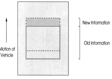
This chapter provides a general overview of video compression. The first part of the chapter discusses the three elements of video compression, which were briefly mentioned in Chapter 1, in greater detail. More details about video compression can be found in [1,2]. The second part of this chapter briefly describes the general approach used by typical compression standards. Motion of Vehicle New Information Old Information Ocean Floor

Figure 2-1: Collection of two subsequent frames by the UUV

2.1 Representation

The first step in compressing and coding a video sequence is to find a compact way to represent the video sequence. The video sequence obtained by the UUV, at 30 frames per second, 640x480 pixels, and 8 bits per pixel, contains both temporal and spatial redundancies. The temporal redundancies exist because the video sequence does not usually change very much from

(11)

one frame to the next. For example, Figure 2-1 demonstrates the collection of two subsequent frames. The solid line represents the current frame, and the dashed line represents the new frame. As Figure 2-1 indicates, a large portion of the new frame overlaps with the old frame, and only the top region of the new frame contains any new information. Spatial redundancies exist because each pixel within a given frame tends to be highly correlated with its surrounding pixels.

2.1.1 Temporal Redundancies

Temporal redundancies exist in video sequences because neighboring frames have more similarities than differences. Motion estimation exploits the temporal redundancies. Instead of transmitting each frame individually, motion estimation involves transmitting two translational vectors and the error. The translational vectors, an x-vector which describes the horizontal motion, and a y-vector which describes the vertical motion, predict the current frame from the previous frame. The error, which is the difference between the predicted frame and the current frame, is minimal if the prediction model is accurate. Motion estimation reduces the amount of information transmitted because each translational vector is represented by a relatively small number of bits, and the error usually contains few non-zero coefficients.

However, not all frames are predicted from past frames. It is necessary to encode a frame without reference to any other frames if it is the beginning of a video sequence or if a scene change occurs in the video sequence. In both cases, motion estimation leads to large errors. However, for an underwater video sequence, rapid scene changes do not occur because the UUV

(12)

travels slowly and the ocean floor changes gradually. In particular, for an underwater video sequence, only the first frame needs to be encoded independently from the other frames.

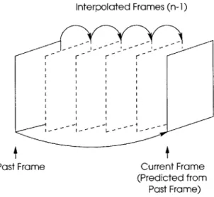
Interpolated Frames (n-1)

Past Frame Current Frame (Predicted from

Past Frame)

Figure 2-2: Interpolation of the skipped frames

If a video sequence is not changing rapidly from one frame to the next, interpolation

further exploits the temporal redundancies by encoding every nth frame instead of every frame. The rate at which the video sequence changes determines (n-1), the number of frames to be skipped. The nth frame, the current frame, is encoded by using motion estimation. The skipped (n-1) frames are recovered by interpolating between the past frame and the current frame, as shown in Figure 2-2. Since an underwater video sequence is obtained from a slow moving UUV, interpolation allows many frames to be skipped without considerably degrading the quality of the underwater video sequence.

2.1.2 Spatial Redundancies

Redundancies exist in the spatial dimension as well. Often, a pixel within a given frame is correlated with the surrounding pixels. For example, in a region of constant intensity, all of the pixels in the area have the same value. Since the ocean floor consists mainly of sand, which is

(13)

fairly uniform in color, an underwater video sequence usually contains many areas of virtually constant intensity. The Discrete Cosine Transform (DCT) exploits the spatial correlations inherent within each frame by transforming each 8x8 block in the frame from the spatial domain to the frequency domain. The DCT decorrelates the coefficients from one another and effectively consolidates most of the energy into the lower frequency coefficients.

2.1.3 Intra Blocks and Inter Blocks

There are two types of blocks, intra blocks and inter blocks. An intra block is the DCT of

an 8x8 block of original data. The DCT consolidates most of the energy into the lower

frequencies because the pixels in each 8x8 block of original data tend to be highly correlated. An inter block is the DCT of an 8x8 block that represents the error. Assuming that the motion estimation is accurate, each 8x8 block of error contains few coefficients with large amplitudes. As a result, the DCT of a sparse 8x8 block leads to another sparse 8x8 block.

Each frame in the video sequence is broken down into intra blocks and inter blocks. Since the first frame of a video sequence contains a new set of data, it is represented entirely by intra blocks. Subsequent frames are represented by a combination of intra and inter blocks. Blocks that contain new information are treated as intra blocks and encoded in their entirety. Blocks that can be predicted from past frames are treated as inter blocks, and the error represented by each inter block is encoded.

2.2 Quantization

Quantization involves assigning every possible value that a DCT transform coefficient can take on to a reconstruction level because only a finite number of reconstruction levels can be

(14)

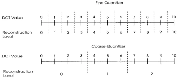
represented with a finite number of bits. Only the magnitude of each value is quantized where the sign of each value is transmitted separately. In general, coarser quantizers retain less information than fine quantizers. Also, coarse quantizers require a fewer number of bits to represent the amplitude of a reconstruction level because there are fewer levels.

Fine Quantizer DCT Value 0 1 2 3 4 5 6 7 8 9 10 Reconstruction Level DCT Value Rcontru ct±ion r o l 2 3 4 5 6 7 8 9 10 Coarse Quantizer o 1 2 3 4 5 6 7 8 9 10 Level 0 1 2

Figure 2-3: Reconstruction levels for a fine quantizer and a coarse quantizer

Figure 2-3 displays the reconstruction levels for a fine quantizer and for a coarse quantizer. The dashed lines delineate the boundaries between the reconstruction levels. The first thing to

note is that coarse quantizers quantize more transform coefficients to zero because there are fewer

reconstruction levels. For example, the fine quantizer in Figure 2-3 quantizes all values between 0 and 0.5 to reconstruction level 0, whereas the coarse quantizer in Figure 2-3 quantizes all values between 0 and 3.5 to reconstruction level 0.

Not only do coarse quantizers quantize more transform coefficients to zero, coarse quantizers also quantize values to a smaller number of reconstruction levels. As a result, the amplitude of the reconstruction level tends to be smaller for coarse quantizers. For example, the

(15)

fine quantizer in Figure 2-3 quantizes a value of 9.2 to reconstruction level 9. On the other hand, the coarse quantizer in Figure 2-3 quantizes a value of 9.2 to reconstruction level 2.

There are a total of 31 different quantization levels, ranging from Quantizer 1, the finest quantizer, to Quantizer 31, the coarsest quantizer. The quantizer is chosen such that the bit-rate remains at 10 kbps at all times. If the bit-rate dips below 10 kbps, more information can be transmitted, and the current frame is quantized with a finer quantizer. If the bit-rate exceeds 10

kbps, less information can be transmitted, and the current frame is quantized with a coarser quantizer. After quantization, the amplitude of the reconstruction level of the quantized DCT transform coefficient is transmitted. An additional bit, which indicates the sign, is transmitted along with each amplitude.

27 29 35 38 46 56 69 83 23 24 25 26 27 28 29 30 26 27 29 34 38 46 56 69 22 23 24 25 26 27 28 29 26 27 29 32 35 40 48 58 21 22 23 24 25 26 27 28 22 26 27 29 34 35 40 48 20 21 22 23 24 25 26 27 22 22 26 27 34 34 37 40 19 20 27 22 23 24 25 26 19 22 26 27 29 34 34 38 18 19 20 21 22 23 24 25 16 16 22 24 27 29 34 37 17 18 19 20 21 22 23 24 8 16 19 22 26 27 29 34 16 17 18 19 20 21 22 23 Intra Weighting Matrix Inter Weighting Matrix

Figure 2-4: Weighting matrices used for quantization

Prior to quantization, entry by entry division with the appropriate weighting matrix is applied to each 8x8 block of transform coefficients. The left-hand matrix shown in Figure 2-4 is applied to intra blocks, and the right-hand matrix shown in Figure 2-4 is applied to inter blocks. For both matrices, the bottom left-hand corner represents the low frequencies and the upper right-hand corner represents the high frequencies. Both the intra weighting matrix and the inter

(16)

reduce the magnitude of the transform coefficients in the higher frequencies. The weighting matrices effectively cause more of the higher frequency transform coefficients to be quantized to zero. This is desirable because the human visual system is less sensitive to high frequencies.

Although the quantization process discards information, so long as the step size between the reconstruction levels is small enough, the degradation goes unnoticed by the human viewer. This is because the human visual system is not sensitive to small changes in the amplitude of the reconstruction level.

2.3 Coding the Quantized Transform Coefficients

After quantization, a codebook assigns a codeword to each quantized transform coefficient. By employing several encoding schemes, such as runlength encoding, joint event coding and Huffman coding, significant reductions of the bit-rate can be achieved.

2.3.1 Runlength Encoding

Runlength encoding exploits the fact that most of the transform coefficients in each block are zero. Instead of encoding the amplitude of the transform coefficient at each of the 64 positions in the 8x8 block, runlength encoding only encodes the non-zero coefficients by transmitting two

parameters, the amplitude and the runlength from the previous non-zero coefficient. The

runlength is defined to be the number of zeroes between subsequent non-zero coefficients. The position of the current non-zero coefficient is determined from the runlength. The addition of the runlength and the starting position, i.e. the position of the previous non-zero coefficient, specifies the position of the last zero in the run. Thus, the addition of the runlength, the starting position and an additional one establishes the position of the current non-zero coefficient. The position of

(17)

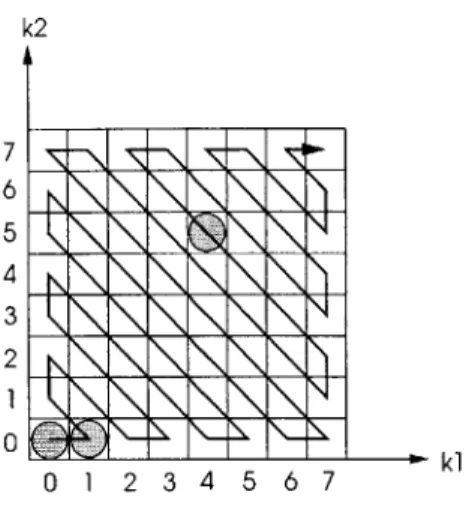
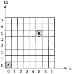
the next non-zero coefficient is calculated by updating the starting position with the current position. The runlength path must be specified when using runlength encoding because there are several paths which can be taken. All experiments in this thesis use the zig-zag scan shown in Figure 2-5.

k2

Starting Position 64

kl

Starting Position 0

Figure 2-5: Location of each starting position, and the zig-zag path

In addition, since the starting position is defined to be the position of the previous non-zero coefficient, runlength encoding requires that the starting position for the first non-non-zero coefficient in each 8x8 block be defined. At the beginning of each block, runlength encoding initializes the starting position to zero. As shown in Figure 2-5, starting position 0 occurs right before the (0,0) position in the 8x8 block. Hence, the runlength of the first non-zero coefficient is the number of zeroes between starting position 0 and the first non-zero coefficient. The runlength

(18)

k2 7 6 5 4 3 2 1 0 1 2 3 4 5 6 7

Figure 2-6: Zig-zag scanning used for runlength encoding

Runlength encoding treats intra and inter blocks slightly differently. For an intra block, since most of the energy is concentrated in the lower frequencies and the DC component is almost always non-zero, runlength encoding encodes the amplitude of the DC component every time. As a result, the runlength of the first event is excluded, and the starting position is initialized to 1. For example, the sequence of events to be encoded for Figure 2-6 as an intra block is shown below. The EOB (End-of-Block) signifies that the rest of the transform coefficients in the block are zero.

[1] amplitude of (0,0) coefficient; [2] runlength 0; [3] amplitude of (1,0) coefficient; [3] runlength 44; [5] amplitude of (4,5); [6] EOB.

For inter blocks, unlike intra blocks, there is no guarantee that the DC coefficient is non-zero because inter blocks tend to be sparse. Runlength encoding encodes the runlength of the first non-zero coefficient. The sequence of events to be coded for Figure 2-6 as an inter block is shown on the following page.

(19)

runlength 0; amplitude of runlength 0; amplitude of runlength 44; amplitude of EOB. (0,0) coefficient; (1,0) coefficient; (4,5);

2.3.2 EOB versus Last Bit

It is important to note that the EOB character is necessary because it indicates when one block has ended and when the next block begins. An alternate approach, last bit encoding, inserts an additional bit after each non-zero coefficient. The additional bit acts like a flag and specifies whether or not there are any additional non-zero coefficients in the block. The last bit is set to '1' when the rest of the transform coefficients in the block are zero. Otherwise, the last bit is set to '0'. If last bit encoding is used, the sequence of events to be coded for Figure 2-6 as an inter block is shown below. [1] [2] [3] [4] [5] [6] [7] [8] [9] runlength 0; amplitude of (0,0) coefficient; last 0; runlength 0; amplitude of (1,0) coefficient; last 0; runlength 44; amplitude of (4,5); last 1;

2.3.3 Joint Event Coding

Each non-zero transform coefficient has two parameters associated with it: the amplitude

and the runlength. The straightforward approach encodes each parameter of the transform

coefficient separately where one codebook maps the amplitude to one codeword and another

[1] [2] [3] [4] [5] [6] [7]

(20)

codebook maps the runlength to another codeword. Joint event coding, instead, treats the amplitude and the runlength as one event and maps the pair to a single codeword. Joint event coding leads to reductions in the bit-rate because it allows the correlations between the amplitude and the runlength to be exploited.

Joint event coding is not limited to two-dimensional codebooks. Three-dimensional codebooks achieves even greater compression if all three parameters are correlated. If the last bit encoding scheme is used, it is advantageous to treat the amplitude, the runlength, and the last bit as a joint event. In the case of underwater video sequences, the amplitude, the runlength, and the last bit are highly correlated with one another. Section 3.2 explains why in greater detail.

Through joint event coding, no additional bits are required to transmit the last bit because the last bit is transmitted as part of each event. Once the last event in a block occurs, decoding the codeword immediately reveals that it is the end of the block. On the other hand, the EOB scheme requires that an additional codeword be transmitted at the end of each block. Since the EOB scheme usually results in higher bit-rates, this thesis uses last bit encoding.

2.3.4 Huffman Coding

The bit-rate can be reduced further by using variable length codes (VLC) where each codeword has a different length. The shortest codewords are assigned to the most likely events, and the longest codewords are assigned to the least likely events. Huffman coding takes the probability distribution of all of the possible events that can occur, and based on the distribution, assigns a codeword to each event. The probability distribution determines the length of the codewords.

(21)

2.4 Conventional Coding Approaches

Typical compression algorithms, such as H.263 and MPEG, allocate one codebook for inter blocks and another codebook for intra blocks because the probability distributions of the intra blocks and the inter blocks are inherently different. The quantized transform coefficients of an intra block are concentrated in the lower frequencies, while the transform coefficients of an inter block are sparse. Each codebook is designed using runlength encoding, joint event coding,

(22)

Chapter 3 Quantizer/Position-Dependent Encoding

This chapter defines Quantizer/Position-Dependent Encoding and its advantages over standard compression approaches. First, this chapter begins by defining and describing the

benefits of Position-Dependent Encoding (PDE). This chapter then proceeds to describe

Quantizer/Position-Dependent Encoding(QPDE) and its advantages by expanding on the idea of

PDE.

3.1 Position-Dependent Encoding

As described in Chapter 2, standard compression algorithms encode inter blocks with one codebook and intra blocks with another codebook. Instead of using one codebook to map each event that occurs in a block to a codeword, PDE employs a different codebook for each starting position in the block. That is, the starting position determines which codebook is used to map the event to a codeword. Since there are two types of blocks, intra and inter, and there are 65 starting positions in each block, PDE requires 130 codebooks.

PDE codebooks are designed with the same principles outlined earlier in Chapter 2. PDE

uses both joint event coding and Huffman coding to take advantage of the correlations that exist between the amplitude, the runlength, and the last bit at each starting position. As a result, the shortest codewords are assigned the most likely events and the longest codewords are assigned to the least likely events.

(23)

3.2 Motivation For Position-Dependent Encoding

This section describes how the statistics of the runlength, the amplitude, the last bit, and the runlength range all vary as a function of the starting position. Unlike standard compression algorithms, PDE is sensitive to the starting position of the transform coefficient and effectively exploits the correlations that exist between the starting position and the runlength range, the

amplitude, the runlength, and the last bit.

k2 7 6 5 4 3 2 Skl 0 1 2 3 4 5 6 7

Figure 3-1: 8x8 block of quantized transform coefficients

The runlength range varies as a function of starting position. For example, at starting position A in the block shown in Figure 3-1, representing the runlength requires a minimum of six bits because the runlength can take on any value between 0 and 63. At starting position B in Figure 3-1, representing the runlength requires only four bits, two bits less than at starting

position A, because the runlength can only take on a value between 0 and 12. Standard

compression algorithms must always assume that the runlength ranges from 0 to 64 because they are insensitive to the starting position. However, PDE, which is sensitive to starting position, exploits the runlength range.

(24)

The statistics of the amplitude and the statistics of the runlength vary as a function of the starting position as well. For reasons described in Chapter 2, the lower frequency region contains more non-zero coefficients. In the higher frequency region, the non-zero coefficients are rare and far apart. Thus, the amplitude and the runlength are highly correlated with the starting position. For example, at starting position A, one expects either a large or small amplitude, depending on the block type, and a short runlength. At starting position B, one expects a small amplitude and a long runlength.

Not surprisingly, the statistics of the last bit is highly correlated with the starting position as well. If a non-zero coefficient occurs in the lower frequency region, it is not likely to be the last non-zero coefficient since there tends to be many other non-zero coefficients in this region. However, if a non-zero coefficient occurs in the higher frequency region, it is quite likely that it is the last non-zero coefficient since there are few non-zero coefficients in the high frequency region.

Clearly, the statistics of the runlength, the amplitude and the last bit all vary as a function of the starting position. The most likely event at starting position A is quite different from the most likely event at starting position B. Thus, the shortest codeword should be assigned to one event at starting position A and to another event at starting position B. For this reason, it is advantageous to utilize PDE, an encoding scheme which is sensitive to the starting position. PDE encodes each starting position with a different codebook and assigns the shortest codeword to the most likely event at each starting position. Standard compression algorithms are limited to assigning the shortest codewords to the most likely event in the entire block. See [3, 4, 5] for more information about PDE.

(25)

3.3 Quantizer/Position-Dependent Encoding

As described earlier in Chapter 2, each block of data is quantized before it is encoded into

a bit stream. Standard compression algorithms encode each block of quantized transform

coefficients with the same codebook. Quantizer/Position-Dependent Encoding (QPDE) uses a separate set of position-dependent codebooks for each quantizer. Since there are 31 different levels of quantization, and there are 130 codebooks in each set of position-dependent codebooks,

QPDE requires a total of 4,030 codebooks.

3.4 Motivation for QPDE

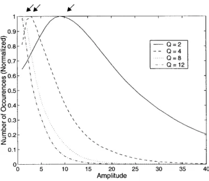
Not only do the statistics of the amplitude, the runlength and the last bit vary with the starting position, they vary with the quantizer as well. For both intra and inter blocks, the statistical differences between the quantizers decrease with increasing quantization. This is because coarse quantizers lead to fewer non-zero coefficients and smaller amplitudes. Section 2.2 explains the reason for this in greater detail. As a result, as the quantizer becomes coarser, the most likely event becomes smaller, and the statistics change. However, after a certain point, the statistical differences begin to disappear because almost everything is quantized to zero.

Figure 3-2 shows the collected statistics of the amplitude for four different quantization levels: 2, 4, 8, and 12. Quantizer 2 is the finest quantizer and Quantizer 12 is the coarsest quantizer. As the arrows in Figure 3-2 indicate, as the quantizer becomes coarser, the statistics change and the most likely event shifts to the left.

(26)

0 5 10 15 20 25 30 35 40 Amplitude

Figure 3-2: Number of occurrences of each amplitude for four different quantizers

Since the most likely event changes as a function of the quantizer, it is advantageous to use QPDE which employs a different set of position-dependent codebooks for each quantizer to ensure that the most likely event is assigned to the shortest codeword. For each quantizer, QPDE uses position-dependent codebooks because regardless of the quantizer, the statistics change as a function of the starting position.

(27)

Chapter 4 Codebook Design

In designing quantizer/position-dependent codebooks to encode an underwater video sequence, many practical issues arise. First, this chapter discusses the issue of codebook design. Implementation of quantizer/dependent codebooks requires a separate set of position-dependent codebooks for each of the 31 quantizers, and each set of position-position-dependent codebooks requires 130 codebooks. QPDE calls for a total of 4,030 codebooks. The impracticality of implementing of 4,030 codebooks demands that the number of codebooks be reduced to a reasonable number. This chapter presents an effective method for scaling down the number of codebooks.

Next, this chapter addresses the issue of codebook size. Each codebook is

three-dimensional where each event represents the amplitude, the runlength and the last bit. There are 1,024 possible levels for the amplitude, up to 65 possible runlengths, and 2 possible values for the last bit, either '0' or '1'. Each codebook contains up to 133,120 entries. Once again, the impracticality of implementing 4,030 codebooks with 133,120 events each becomes a problem. This chapter provides a solution which allows the number of events in each codebook to be reduced significantly.

4.1 Codebook Allocation

(28)

significantly. Although there are 65 different starting positions in each 8x8 block, many of these starting positions share similar statistics. As a result, by grouping together the starting positions with similar statistics, fewer codebooks are needed.

k2 7 6 5 4 3 2

ILIE I II

k1 0 1 2 3 4 5 6 7

Figure 4-1: One possible grouping for the different positions

The statistical variations between starting positions determine which starting positions should be grouped together. Starting positions in the lower frequency region take on a larger range of values because most of the energy is concentrated in the lower frequencies. On the other hand, starting positions in the high frequency region take on similar values because the transform coefficients are usually very close to zero at higher frequencies. Since there tends to be more variation within each starting position in the lower frequencies, there tends to be more statistical differences between the starting positions in the lower frequencies. As a result, typically, the low frequency starting positions are placed in separate groups and the high frequency starting

positions are grouped together. Figure 4-1 shows one possible grouping where the 65 starting

(29)

contain fewer starting positions and groups in the higher frequencies contain more starting positions.

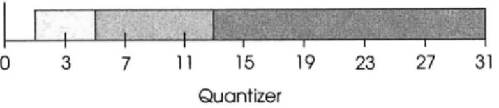
Grouping quantizers with similar statistics cuts down the number of codebooks needed even further. There tends to be more statistical differences between the fine quantizers than coarse quantizers because finer quantizers retain more information than coarser quantizers. In addition, the statistical differences between coarse quantizers disappear because coarse quantizers quantize more of the transform coefficients to zero. Thus, it is reasonable to separate the fine quantizers into different groups and to group the coarse quantizers together. Figure 4-2 demonstrates a plausible grouping of the quantizers.

0 3 7 11 15 19 23 27 31

Quantizer

Figure 4-2: A possible grouping of the 32 different quantizers

With the groupings suggested in Figure 4-1 for the starting positions, and the groupings suggested in Figure 4-2 for the quantizers, the total number of codebooks required by QPDE is reduced from 4,030 to 32. There are four groups of quantizers, and each group demands two sets of position-dependent codebooks, one for intra blocks and another for inter blocks, where each set of position-dependent codebooks contains four codebook.

4.2 Codebook Size

Each three-dimensional codebook encodes the amplitude, the runlength, and the last bit, and contains many events. With an amplitude range between 0 and 1,024, a runlength range

(30)

between 0 and 64, and the last bit, there are a total of 133,120 possible events. Since only a small percentage of these events occur with high probability by only assigning codewords to the events with high probability of occurrence minimizes the number of codewords in each codebook. However, in the off chance that an event that does not have a codeword happens, an escape code is used to encode the event.

4.2.1 Escape Codes

It is necessary to design each codebook such that any event not included in the codebook is still mapped to a unique codeword because no matter how improbable an event is, there is still a chance that it may occur. Each codebook contains an escape code with a corresponding codeword. When an event that does not have a codeword occurs, the codeword for the escape code is transmitted, along with an additional 17 bits. The 17 bits specify the amplitude, the runlength, and the last bit. The first 10 bits represent the amplitude of the event, the next 6 bits represent the runlength and the 17th bit indicates whether or not the current transform coefficient is the last non-zero coefficient in the block. Clearly, the use of escape codes can be quite detrimental to the bit-rate. Fortunately, events not included in the codebook rarely occur, and the bit-rate is not significantly increased by limiting the size of each codebook to include only the most likely events.

4.2.2 Limiting the Codebook Size

One approach which can be used to reduce the codebook size is to limit the number of codewords per codebook. When only the most likely events are included in the codebook, all other events are escape coded. The sum of the probabilities of all the events to be escape coded

(31)

determines the probability of the escape code. The Huffman algorithm designs the codebook based on the probability distribution of only the most likely events and the escape code.

4.2.3 Limiting the Codeword Length

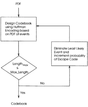
The size of the codebook can also be limited by specifying the maximum length of any one codeword in the codebook. The bit-rate suffers when the codewords become too long. Thus limiting the maximum length of any one codeword prevents any codeword from becoming too long. The simple algorithm outlined in Figure 4-3 limits the maximum length of the codeword. First, the Huffman algorithm designs a codebook based on the probability distribution of all the events. If the length of any codeword exceeds the maximum length, the probability distribution is updated by eliminating the least probable event and adding its probability to the probability of the escape code. The entire process is repeated until the length of each codeword in the codebook does not exceed the desired maximum length.

PDF

Yes

Codebook

(32)

4.3 All Zero Blocks

When very coarse quantizers are used, an entire block of zero coefficients becomes quite

likely. However, this causes potential problems because when there is a block of zero

coefficients, no events are encoded for the current block and the events of the next block are assumed to be the events of the current block. One way to avoid this problem is to include an additional codeword, ZERO, which indicates when there is a block of all zero coefficients. Since the event ZERO only occurs when using the codebook for starting position 1 for an intra block, and the quantizer-dependent codebooks for starting position 0 for an inter block, these codebooks contain a codeword for the event ZERO. It is not necessary to include the event ZERO in the other codebooks because they are only used if there is at least one other non-zero coefficient in the 8x8 block.

(33)

Chapter

5 Experiments

This chapter describes the steps taken to find a set of quantizer/position-dependent codebooks which minimizes the number of codebooks, the number of codewords in each codebook, and the bit-rate. The first step is to derive the joint probability distribution of the events for each starting position and quantizer, where each event represents the amplitude, the runlength, and the last bit. The next step is to establish the trade-off between the number of codebooks and the bit-rate by determining the advantage of having one grouping of the starting positions and the quantizers over another grouping. The final step is to determine the trade-off between the number of codewords in each codebook and the bit-rate by evaluating the performance of various sets of quantizer/position-dependent codebooks which each contain a different number of codewords.

5.1 Collecting Statistics

The performance of a particular grouping of the starting positions and the quantizers is assessed by encoding a test sequence with the corresponding set of quantizer/position-dependent codebooks. Each codebook in the set is designed by Huffman coding the appropriate joint probability distribution. Hence, before any codebooks can be designed, the joint probability distribution for each starting position and quantizer must be determined. This proves to be quite simple. By collecting statistics from a series of training sequences and tallying the number of times each event occurs, the resulting histogram is roughly proportional to the joint probability

(34)

In this thesis, statistics were collected from six training sequences which were acquired from live underwater video sequences provided by Draper Laboratory. The training sequences, selected such that a variety of ocean floor scenarios were included, consisted of 1000 frames each. The training sequences were encoded with the following twelve quantization levels: 1, 2, 3, 4, 5,

7, 8, 9, 10, 12, 16, and 20. For each quantization level, a set of statistics were collected for intra

blocks and another set of statistics were collected for inter blocks. Each set of statistics for a given block type contains 65 histograms, one for each starting position in the block.

Unfortunately, the histogram of the collected statistics does not provide a complete description of the joint probability distribution. Many events occur with very small probabilities. Consequently, the improbable events rarely appear in the histogram, inaccurately suggesting that these events occur with zero probability. To account for the discrepancy between the collected statistics and the joint probability distribution, the probability of the events that do not occur in the training sequences must be estimated.

~I) - -Collected Statistics - - - Estimated Events 0 0 E 0 i 0 512 1028 Amplitude

(35)

This thesis estimates the probabilities of the missing events by assuming that all of the unlikely events occur with equal probability. The solid line in Figure 5-1 outlines a histogram of the amplitude for a particular runlength and last bit. As one can see from Figure 5-1, events with an amplitude greater than 512 never happen in the training sequence. To approximate the probability of the events with an amplitude of 512 or greater, the histogram is extended uniformly to include all of the possible amplitudes. The dashed line in Figure 5-1 represents the updated histogram. Normalization of the updated histogram results in an approximation of the joint probability distribution of the events.

5.2 Reducing the Number of Codebooks

This thesis uses two techniques to reduce the number of codebooks. The first technique groups together starting positions with similar statistics. It then assigns one codebook to each group of starting positions instead of one codebook to each starting position. The second technique, conceptually very similar to the first technique, groups together quantizers with similar statistics. Then, it allocates one set of position-dependent codebooks to each group of quantizers instead of allocating one set of position-dependent codebooks to each quantizer.

This section first examines which grouping of the starting positions leads to a minimal number of codebooks and a reasonable bit-rate. Then this section investigates which grouping of the quantizers results in a minimal number of sets of position-dependent codebooks without sacrificing bit-rate. Finally, once the grouping of the quantizers has been decided, this section explores whether a different grouping of the starting positions for each group of quantizers produces further optimizations.

(36)

5.2.1 Grouping the Positions

Grouping together statistically similar starting positions and assigning one codebook to each group reduces the number of position-dependent codebooks without affecting the bit-rate. This is because statistically similar starting positions have similar codebooks. In order to determine which starting positions should be grouped together, the relationship between the statistics of each starting position must be established.

For an intra block, the starting positions in the lower frequencies are more likely to be statistically different while the starting positions in the higher frequencies are more likely to be statistically alike. This is true for two reasons. First, as described in Section 2.1, most of the energy is consolidated in the lower frequencies. Second, the intra weighting matrix, shown in Figure 2-4, magnifies the amplitudes in the lower frequencies and suppresses the amplitudes in the higher frequencies. The DC component typically contains the largest fraction of the total energy and takes on the widest range of values. Each subsequent frequency component contains a smaller portion of the total energy and takes on a smaller range of values.

Consequently, the statistical differences between starting positions in the lower frequencies are more likely to be substantial because starting positions in the lower frequencies contain large variations. On the other hand, the statistical differences between the starting positions in the higher frequencies are more likely to be inconsequential because the starting positions in the higher frequencies contain fewer variations. Thus, the statistical differences between starting positions decrease with increasing frequency.

Since most of the statistical differences exist in the lower frequencies for an intra block, it is advantageous to allocate most of the position-dependent codebooks to the starting positions in the lower frequencies. For example, if four position-dependent codebooks are to be used, the

(37)

optimal grouping assigns one codebook to each of the starting positions 0, 1, and 2, and the fourth codebook to starting positions 3 through 64.

An alternative grouping of the starting positions, which is suggested by Figure 4-1, allocates the first codebook to starting position 0, the second to starting positions 1 through 5, the third to starting positions 6 through 20, and the fourth to starting positions 21 through 64. However, this grouping is not used because the weighting matrix causes statistical differences between the starting positions decrease with increasing frequency.

For an inter block, the starting positions in the lower frequency region tend to be statistically different while the starting positions in the higher frequency region tend to be statistically similar. This is because the inter weighting matrix magnifies the amplitudes in the lower frequency region and causes the statistical differences between the starting positions to become more prominent. The inter weighting matrix also suppresses the amplitudes in the higher frequency region and causes the statistical differences between the starting positions to disappear.

Since the starting positions in the lower frequencies contain more statistical differences,

PDE allocates most of the position-dependent codebooks to the starting positions in the lower

frequencies. For example, if four position-dependent codebooks are to be used to encode an inter block, the optimal grouping allocates one codebook to each of the starting positions 0, 1, and 2, and the fourth codebook to starting positions between 3 through 64.

The following experiment determines how many position-dependent codebooks should be implemented by establishing the trade-off between the number of position-dependent codebooks and the bit-rate. Eight sets of position-dependent codebooks were designed by Huffman coding the appropriate joint probability distributions. They are listed in column 1 of Table 5-1. The second column of Table 5-1 lists the number of codebooks in each set. The third column indicates

(38)

the breakdown of the groups for each set. For example, Set A contains eight codebooks where one codebook is allocated to each of the starting positions 0, 1, 2, 3, 4, 5, and 6. The eighth codebook encodes all of the starting positions between 7 and 64. Each set, B through H, contains one less codebook than the previous set.

Number of Groups of Positions codebooks Set A 8 0, 1, 2, 3, 4, 5, 6, 7-64 Set B 7 0, 1, 2, 3, 4, 5, 6-64 Set C 6 0, 1, 2, 3, 4, 5-64 Set D 5 0, 1, 2, 3, 4-64 Set E 4 0, 1, 2, 3-64 Set F 3 0, 1, 2-64 Set G 2 0, 1-64 SetH 1 0-64

Table 5-1: The number of codebooks and the grouping of the starting

positions for Set A through Set H

Each of the eight sets of position-dependent codebooks was applied to six different test sequences. The test sequences, which were obtained from the underwater video sequences provided by Draper Laboratory, were not included in the training sequences. Table 5-2(a) displays the bit-rate, in kbps, required to encode the intra blocks of each test sequence. Table

5-2(b) displays the bit-rate, in kbps, required to encode the inter blocks of each test sequence. The

last column in both Table 5-2(a) and Table 5-2(b) list the average percentage gain each set of position-dependent codebooks achieves over Set H, which is not position-dependent. The best grouping is determined separately for intra and inter blocks.

(39)

Test 1 Test 2 Test 3 Test 4 Test 5 Test 6 % Gain SetA 4.72 5.50 5.58 5.35 5.52 5.34 6.74 SetB 4.73 5.50 5.58 5.35 5.52 5.34 6.71 SetC 4.75 5.50 5.58 5.36 5.53 5.35 6.54 Set D 4.77 5.50 5.58 5.37 5.51 5.37 6.49 SetE 4.80 5.54 5.59 5.39 5.54 5.38 6.12 SetF 5.04 5.63 5.74 5.52 5.67 5.50 3.49 SetG 5.04 5.72 5.77 5.56 5.72 5.53 2.93 SetH 5.25 5.90 5.92 5.71 5.89 5.68 0.00 (a)

Test I Test 2 Test 3 Test 4 Test 5 Test 6 % Gain

SetA 6.75 9.69 10.26 9.88 9.31 12.00 8.51 SetB 6.76 9.70 10.28 9.90 9.32 12.01 8.36 SetC 6.76 9.72 10.29 9.91 9.33 12.06 8.21 SetD 6.76 9.74 10.31 9.94 9.38 12.10 8.00 SetE 6.77 9.75 10.32 9.95 9.38 12.15 7.89 SetF 6.75 9.79 10.36 10.00 9.39 12.19 7.58 SetG 6.82 9.94 10.53 10.15 9.55 12.40 6.13 SetH 6.78 10.69 11.38 10.93 10.23 13.26 0.00 (b)

Table 5-2: (a) The bit-rate required to encode the intra blocks. (b) The

bit-rate required to encode the inter blocks.

The results of the experiment shown in Table 5-2(a) determine how the starting positions for an intra block should be grouped. Set A, which contains 8 codebooks, achieves an average gain of 6.74% over Set H. Set E, which has 4 codebooks, obtains a gain of 6.12% over Set H. Set F, which contains 3 codebooks, realizes a gain of 3.49% over Set H. The average gain is only reduced by 0.62% when the number of codebooks is reduced from 8 to 4. However, when the number of codebooks is cut back from 8 to 3, the average gain decreases by another 2.63%. Thus,

(40)

for an intra block, the starting positions should be separated into the four groups suggested by Set

E. This is because increasing the number of codebooks beyond four does not improve the bit-rate

significantly, and decreasing the number of codebooks below four worsens the bit-rate considerably.

The results of the experiment shown in Table 5-2(b) establish the best grouping of the starting positions for an inter block. Reducing the number of position-dependent codebooks from eight to four codebooks diminishes the average gain of PDE by 0.62%. The average gain decreases by another 0.29% when the number of position-dependent codebooks is reduced to three codebooks. Since a 0.29% decrease in the average gain is significant in comparison to the a

0.62% decrease in the average gain, the starting positions for an inter block should be separated

into the four groups suggested by Set E.

5.2.2 Grouping the Quantizers

Another method used to cut back the number of codebooks is to group quantizers with similar statistics together. Each group of quantizers is then assigned one codebook. As long as quantizers with similar statistics are grouped together, the bit-rate is not significantly affected because quantizers with similar sets of statistics also have similar sets of position-dependent codebooks.

The statistical differences between quantizers decrease with increasing quantization. The reasons for this was explained earlier in Section 3.4. For example, one reasonable grouping, which was suggested earlier in Figure 4-2, allocates one set of position-dependent codebooks to

(41)

Quantizer 1, a second set to Quantizers 2 through 4, a third set to Quantizers 5 through 12, and a fourth set to Quantizers 13 through 31.

0 5 10 15 20 Amplitude (a) 25 30 35 40 Amplitude (b) 10 15 20 25 30 35 Amplitude (C) 40

Figure 5-2 : _{Probability distribution for: (a) Quantizers 1, 2, 3, and 4. (b) Quantizers 4,} 5, 7, and 8. (c) Quantizers 8, 12, 16, and 20

When dividing the quantizers into groups, there are two requirements that should be satisfied by each quantizer within a given group. First, it is desirable for the most likely event of each quantizer in a given group to be the same. This ensures that the shortest codeword is always assigned to the most likely event. Second, it is desirable for the probability distribution of each quantizer in the group to have approximately the same shape. This guarantees that the codeword assigned to each event minimizes the average bit-rate. Consequently, a careful examination of the

0.8 Q1Q 002 0.6- 04 0.4 03 0.2 ..._{.. ...}

(42)

probability distribution of each quantizer leads to the best grouping for the quantizers. Figure 5-2 shows the probability distribution of the amplitude for a runlength of 0 and a last bit of 0 for each of the following quantizers: 1, 2, 3, 4, 5, 7, 8, 12, 16, and 20. Figure 5-2 reveals how to group several of the quantizers. Figure 5-2(a) implies that Quantizer 1 should not be grouped with any other quantizers because its probability distribution is unlike the probability distribution of any other quantizer. For example, the most likely event for Quantizer 1 is an amplitude of 10, a runlength of 0, and a last bit of 0. However, this event tends to be one of the less likely events for all of the other quantizers.

Table 5-2(b) suggests that Quantizers 5 through 7 should form another group because the

quantizers have almost identical probability distributions. Not only do the probability

distributions of the quantizers share the same shape, the most likely event for each quantizer is also the same. Although the probability distribution of Quantizer 6 is not shown, statistics change gradually from one quantizer to the next, and it is logical to assume that the statistics of Quantizer

6 are very similar to the statistics of Quantizer 5 and Quantizer 7.

Since Quantizer 8, Quantizer 12, Quantizer 16, and Quantizer 20 have the same shape and most likely event, Figure 5-2(c) recommends that Quantizers 8 through 31 be grouped together. The similarities between the probability distributions of Quantizer 8, Quantizer 12, Quantizer 16, and Quantizer 20 suggest that quantization levels greater than 8 all have approximately the same probability distribution.

Although several of the quantizers can be placed into one of the three groups directly from Figure 5-2, it is not clear where Quantizers 2 through 4 should be placed since their probability distributions are comparable, but their most likely events are different. In order to determine the best grouping for the remaining quantizers, the following experiment was conducted. Five sets of

(43)

quantizer/position-dependent codebooks, Set I through Set V, were designed. Each set was designed from a different set of collected statistics. For example, Set III is obtained by Huffman coding the combined statistics of Quantizers 2 through 3. Table 5-3 specifies which statistics were used to design Set I through Set V.

Quantizers Set I 2 Set II 4 Set III 2,3 Set IV 2,3,4 Set V 4,5,6,7

Table 5-3: Thesets of statistics used to design Set I through Set V

Three test sequences were quantized with Quantizer 2. Then, each quantized test

sequence was encoded with each of the five sets of quantizer/position-dependent codebooks. Columns 2 through 4 of Table 5-4 list the bit-rates achieved by Sets I through V. As expected, Set I, which was designed from the statistics of Quantizer 2 only, achieves the lowest bit-rate for all three test sequences. However, Set III and Set IV both attain bit-rates comparable to the bit-rates achieved by Set I.

Q--2 Q=4

Test 1: Test 2: Test 3: Test 1: Test 2: Test 3:

Set 1 27.63 29.75 29.39 13.91 14.87 14.29

Set 1128.03 30.82 30.21 13.65 14.44 13.92

Set 1128.10 30.39 29.79 16.19 16.86 16.42

SetIV 28.41 30.51 29.96 14.94 15.66 15.20

SetV 29.57 32.75 32.13 13.74 14.47 13.93

(44)

For example, when encoding Test Sequence 1 with Set III instead of Set I, the bit-rate increases by 1.7% from 27.63 kbps to 28.10 kbps. Encoding Test Sequence I with Set IV increases the bit-rate by another 1.1% to 28.41 kbps. Since neither Set III nor Set IV significantly worsen the bit-rate, this experiment suggests that Quantizer 2, Quantizer 3, and possibly Quantizer 4 should be grouped together.

The three test sequences were also quantized with Quantizer 4, and then encoded with each of the five sets of quantizer/position-dependent codebooks. Columns 5 through 7 of Table 5-4 list the bit-rates achieved by Set I through Set V. Naturally, Set II, which is designed from the statistics of Quantizer 4 alone, achieves the lowest bit-rates. Set V obtains bit-rates which are comparable to the bit-rates obtained by Set II. However, Set IV attains bit-rates which are significantly worse. For example, when Set V is used to encode Test Sequence 1, the bit-rate only increases 0.6%. On the other hand, when Set IV is used to encode Test Sequence 1 the bit-rate increases 8.42%. Clearly, Set V is a more optimal grouping than Set IV. As a result, Quantizers 2 through 3 form one group, and Quantizers 4 through 7 form another group. Table 5-5 lists the quantizers contained in each of the final four groups.

Quantizers

Group 1 1 Group 2 2,3

Group 3 4,5,6,7

Group 4 8-31

(45)

5.2.3 Optimal Number of Quantizer/Position Dependent Codebooks

Thus far, the optimal grouping of the starting positions has been determined independently of the quantizer, and the optimal grouping of the quantizers has been determined independently of the starting position. However, the quantizer affects how the statistics vary with the starting position. The statistical differences between the starting positions disappear more quickly as the quantizer becomes coarser since a coarse quantizer discards more events. This suggests that a fine quantizer requires more position-dependent codebooks than a coarse quantizer.

The following experiment was conducted to establish whether or not there is an advantage to varying the number of position-dependent codebooks as a function of the quantizer. A test sequence is quantized with both Quantizer 1, a fine quantizer, and Quantizer 10, a coarse quantizer. Then, the finely quantized test sequence, T1Q1, and the coarsely quantized test sequence, T1Q10, are each encoded with separate sets of position-dependent codebooks, Set A through Set H. Each set contains a different number of codebooks. Table 5-1 specifies the number of codebooks and the grouping of the starting positions for each set.

Number of T1Q1 _T1Q10 Codebooks Set A 8 71.10 6.22 SetB 7 71.63 6.25 SetC 6 72.08 6.26 SetD 5 72.51 6.27 SetE 4 72.73 6.27 SetF 3 73.47 6.27 SetG 2 74.20 6.31 SetH 1 76.67 6.66