Computer vision uncovers predictors of physical urban change
The MIT Faculty has made this article openly available.
Please share
how this access benefits you. Your story matters.
Citation
Naik, Nikhil et al. “Computer Vision Uncovers Predictors of Physical
Urban Change.” Proceedings of the National Academy of Sciences
114, 29 (July 2017): 7571–7576 © 2017 National Academy of
Sciences
As Published
http://dx.doi.org/10.1073/PNAS.1619003114
Publisher
National Academy of Sciences (U.S.)
Version
Final published version
Citable link
http://hdl.handle.net/1721.1/114987
Terms of Use
Article is made available in accordance with the publisher's
policy and may be subject to US copyright law. Please refer to the
publisher's site for terms of use.
ECONOMIC SCIENCES
COMPUTER
SCIENCES
Computer vision uncovers predictors of physical
urban change
Nikhil Naika,b,1, Scott Duke Kominersc,d,e,f,g,h, Ramesh Raskarb, Edward L. Glaesere,h,i, and C ´esar A. Hidalgoj
aJoint Center for History and Economics, Harvard University, Cambridge, MA 02138;bMedia Lab, Massachusetts Institute of Technology, Cambridge, MA
02139;cSociety of Fellows, Harvard University, Cambridge MA 02138;dHarvard Business School, Boston, MA 02163;eDepartment of Economics, Harvard
University, Cambridge, MA 02138;fCenter of Mathematical Sciences and Applications, Harvard University, Cambridge, MA 02138;gCenter for Research on
Computation and Society, Harvard University, Cambridge, MA 02138;hNational Bureau of Economic Research, Cambridge, MA 02138;iJohn F. Kennedy
School of Government, Harvard University, Cambridge, MA 02138; andjCollective Learning Group, Media Lab, Massachusetts Institute of Technology,
Cambridge, MA 02139
Edited by Jose A. Scheinkman, Columbia University, New York, NY, and approved May 25, 2017 (received for review November 17, 2016) Which neighborhoods experience physical improvements? In this
paper, we introduce a computer vision method to measure changes in the physical appearances of neighborhoods from time-series street-level imagery. We connect changes in the physical appear-ance of five US cities with economic and demographic data and find three factors that predict neighborhood improvement. First, neighborhoods that are densely populated by college-educated adults are more likely to experience physical improvements—an observation that is compatible with the economic literature link-ing human capital and local success. Second, neighborhoods with better initial appearances experience, on average, larger positive improvements—an observation that is consistent with “tipping” theories of urban change. Third, neighborhood improvement corre-lates positively with physical proximity to the central business dis-trict and to other physically attractive neighborhoods—an obser-vation that is consistent with the “invasion” theories of urban sociology. Together, our results provide support for three classical theories of urban change and illustrate the value of using computer vision methods and street-level imagery to understand the physical dynamics of cities.
urban economics | gentrification | urban studies | computer vision | neighborhood effects
F
or more than a century, urban planners, economists,sociol-ogists, and architects have advanced theories connecting the dynamics of a neighborhood’s physical appearance to its loca-tion, demographics, and built infrastructure.
The tipping theory of Schelling (1) and Grodzins (2) suggests that neighborhoods in bad physical condition will get progres-sively worse, whereas nicer areas will get better. Economic theo-ries of urban change at the city level often emphasize population density and education (3–6), and it is natural to hypothesize that agglomeration of human capital will predict neighborhood-level improvements as well. Theories from urban sociology, such as the invasion theory of Burgess (7), however, emphasize locations and social networks, predicting that improvements in a city’s appearance should be spatially clustered, and that improvements should occur both near the central business districts (CBDs) and near other physically attractive neighborhoods.
To test theories of physical neighborhood change, we need to quantify neighborhood appearance at different points in time. Historically, however, methods to quantify neighborhood appearance have not been scalable. The empirical literature on urban appearance, which was pioneered by urban planners such as Lynch (8), Rapoport (9), and Nasar (10), as well as by psy-chologists such as Milgram (11), has relied on interviews, low-throughput visual perception surveys, and manual evaluation of images. Those methods, however, can only be used to collect data on a few neighborhoods and have limited spatial resolution. In the past decade, new data on urban appearance have emerged in the form of “street view” imagery (12). As of 2016, Google Street View has photographed more than 3,000 cities from 106
countries at the street level. Recent approaches to quantify urban appearance, such as those of Rundle et al. (13), Hwang and Sampson (14), and Salesses et al. (15), leverage this large online corpus of street-level imagery but still rely on manual data cura-tion, limiting throughput.
The appearance of street-level imagery sources has been par-alleled by significant advances in the field of computer vision. Tasks such as automatically classifying and labeling images are now much easier, thanks in part to the availability of more com-prehensive training datasets and new machine learning algo-rithms (16). These advances have led to an emerging literature at the intersection between computer vision, urban planning, urban sociology, and urban economics.
In 2011, the Massachusetts Institute of Technology (MIT) Place Pulse project (15) began collecting a massive crowd-sourced dataset on urban appearance by asking people to select images from pairs in response to evaluative questions (such as “Which place looks safer?”). Naik et al. (17) used the Place Pulse data to train a computer vision algorithm called Streetscore that accurately predicts human-derived ratings for the perception of a streetscape’s safety (also see refs. 18 and 19). Using Streetscore, Naik et al. (17) scored more than 1 million images from 21 cities in the northeastern United States, creating the largest
Significance
We develop a computer vision method to measure changes in the physical appearances of neighborhoods from street-level imagery. We correlate the measured changes with neighborhood characteristics to determine which character-istics predict neighborhood improvement. We find that both education and population density predict improvements in neighborhood infrastructure, in support of theories of human capital agglomeration. Neighborhoods with better initial appearances experience more substantial upgrading, as pre-dicted by the tipping theory of urban change. Finally, we observe more improvement in neighborhoods closer to both city centers and other physically attractive neighborhoods, in agreement with the invasion theory of urban sociology. Our results show how computer vision techniques, in combination with traditional methods, can be used to explore the dynamics of urban change.
Author contributions: N.N., S.D.K., E.L.G., and C.A.H. designed research and experiments; N.N., S.D.K., E.L.G., and C.A.H. performed research and experiments; R.R. and E.L.G. con-tributed new analytic tools; N.N., S.D.K., E.L.G., and C.A.H. analyzed data; and N.N., S.D.K., E.L.G., and C.A.H. wrote the paper.
The authors declare no conflict of interest. This article is a PNAS Direct Submission.
Freely available online through the PNAS open access option.
1To whom correspondence should be addressed. Email: [email protected].
This article contains supporting information online atwww.pnas.org/lookup/suppl/doi:10. 1073/pnas.1619003114/-/DCSupplemental.
high-resolution dataset of urban appearance to date. Been et al. (20) used the Streetscore dataset to show that streets with higher Streetscores in New York are more likely to have been designated as historical districts. Harvey and Aultman-Hall (21) examined the skeletal aspects of neighborhoods to show that nar-row streets with high building densities are perceived as safer than wider streets with few buildings. Nadai et al. (22) used Streetscore and mobile phone data to investigate whether safer-looking neighborhoods are more lively.
A
B
C
D
Fig. 1. Computing Streetchange: (A) We calculate Streetscore, a metric for perceived safety of a streetscape, using a regression model based on two image features: GIST and texton maps. We calculate those features from pixels of four object categories—ground, buildings, trees, and sky—which are inferred using semantic segmentation. (B–D) We calculate the Streetchange of a street block as the difference between the Streetscores of a pair of images captured in 2007 and 2014. (B) The Streetchange metric is not affected by seasonal and weather changes. (C) Large positive Streetchange is typically associated with major construction. (D) Large negative Streetchange is associated with urban decay. Insets courtesy of Google, Inc.
Moreover, crowdsourcing and computer vision methods have been used along with street-level imagery to identify geographi-cally distinctive architectural elements (23), develop unique city signatures (24), and predict socioeconomic indicators (25, 26). Taken together, the range of findings illustrates how computer vision methods can be used to improve the quantitative study of urban appearance and space.
In this paper, we create a high-resolution dataset of physical urban change for five major US cities and use it to study the
ECONOMIC SCIENCES
COMPUTER
SCIENCES
Table 1. Summary statistics (N = 2,513)
Variables Description Mean SD Minimum Maximum
Streetscore 2007 Mean Streetscore 2007 of all sampled street 7.757 2.587 1.681 18.930
blocks within a census tract
Streetchange 2007–2014 Mean Streetchange 2007–2014 of all sampled 1.390 0.779 −4.076 6.121
street blocks within a census tract
Adjacent Streetscore 2007 Mean Streetscore 2007 of all 7.787 2.309 2.548 17.240
boundary-adjacent census tracts
Log population density 2000 Log of population density within a census −4.655 1.220 −15.290 −2.480
tract, as reported by the 2000 US Census
Adjacent log population density 2000 Mean of log population density 2000 for all −4.508 0.883 −11.090 −2.730
boundary-adjacent census tracts
Share college education 2000 The share of adults within a census tract 0.254 0.216 0 1
that have a four-year college degree, as reported by the 2000 US Census
Adjacent share college education 2000 Mean of share college education 2000 for all 0.251 0.191 0.115 1
boundary-adjacent census tracts
Distance to CBD The distance of the census tract from the 5.123 2.685 0 9.997
central business district, in miles
determinants of physical improvements in neighborhoods. We use our data to test three theories of urban change. We find that, in agreement with economic theories of human capital agglomer-ation, neighborhoods that are densely populated by highly edu-cated individuals are more likely to experience positive urban change. Also, in agreement with the invasion theory (7) of urban sociology, we find that neighborhoods are more likely to improve in physical appearance when they are proximate to a CBD and/or other neighborhoods perceived as safe. Finally, we find evidence for a weak version of the neighborhood tipping theory (1, 2), as the neighborhoods that had the best appearances at the begin-ning experienced the largest improvements (however, we do not find that neighborhoods with initially low scores deteriorated— they just improved less). Our findings illustrate how computer vision methods, together with demographic and economic data, can be used to study physical urban change.
Data and Methods
We obtained 360◦ panorama images of streetscapes from five
US cities using the Google Street View application programming interface. Each panorama was associated with a unique identifier (“panoid”), latitude, longitude, and time stamp (which specified the month and year of image capture). We extracted an image cutout from each panorama by specifying the heading and pitch of the camera relative to the Street View vehicle. We obtained a total of 1,645,760 image cutouts for street blocks in Balti-more, Boston, Detroit, New York, and Washington, DC,
cap-tured in 2007 (the “2007 panel”) and 2014 (the “2014 panel”).∗
We matched image cutouts from the 2007 and 2014 panels by using their geographical locations (i.e., latitude and longitude) and by choosing the same heading and pitch. This process gave us images that show the same place, from the same point of view,
but in different years (Fig. 1 B–D).†
We calculated the perception of safety—called “Streetscore”— for each image using a variant of the Naik et al. algorithm (17) trained on a crowdsourced study of people’s perception of safety (15) based on 2,920 images from Boston and New York and
∗For the street blocks that lack images for either 2007 or 2014 we completed the 2007
and 2014 panels using images from the closest years for which data were available. As a result, 5% of the images in the 2007 panel are from either 2008 or 2009. Similarly, 12% of the images in the 2014 panel are from 2013.
†We reduced our data to eliminate pairs containing over-exposed, blurred, or occluded
images (for details, seeSI Appendix).
186,188 pairwise comparisons. The Streetscore computation pro-cess included three steps (Fig. 1A). First, we segmented images into four “geometric” classes: ground (which contains streets, sidewalks, and landscaping), buildings, trees, and sky (27). Next, we created feature vectors characterizing each geometric class using two image features: GIST (28) and texton maps (29). Roughly speaking, these features encode the shapes and tex-tures present in an image. Finally, we used the featex-tures of streets and buildings to predict the Streetscore of an image using sup-port vector regression (30). We ignored the features of trees and sky to minimize seasonal effects (weather, time of day, and time of year). The predicted Streetscore of a Street View image ranges from 0 to 25, with 0 being the most unsafe-looking street scene in the sample and 25 the most safe-looking scene. Next, we computed changes in Streetscores between images in the 2007 and 2014 panels, to obtain Streetchange (Fig. 1 B–D). A posi-tive value of Streetchange is indicaposi-tive of upgrading in physical appearance, whereas a negative value of Streetchange is
indica-tive of decline. (For details on the methods, seeSI Appendix.)
We validated Streetchange using three sources: a survey con-ducted on Amazon Mechanical Turk (AMT), a survey of grad-uate students in MIT’s School of Architecture and Planning, and data from Boston’s Planning and Development Authority (BPDA).
Participants gave informed consent for all human subject stud-ies. Experiments were approved by the Massachusetts Institute of Technology’s Committee on the Use of Humans as Exper-imental Subjects (MIT COUHES). The AMT study was con-ducted in accordance with the requirements of MIT COUHES.
We found strong agreement between Streetchange and both (i) human assessments and (ii) new urban development. In the AMT validation, workers were presented two image pairs, drawn from a pool of 1,565, and asked to select the one showing more physical change. The binned ranked scores pro-vided by the AMT workers had a strong correlation with abso-lute Streetchange (Spearman correlation = 72%, P -value < 1 ×
10−5). In the School of Architecture and Planning student
val-idation we presented students with 150 image pairs and asked them to classify images into positive and negative physical change (N = 3). The students agreed with Streetchange in 74% of cases. Finally, we collected building project data from BPDA and corre-lated Streetchange with total new square footage built per square mile (at census-tract level) during the sample period (2012– 2014). We found a significant and positive correlation between Streetchange and new square footage—one SD increase in log
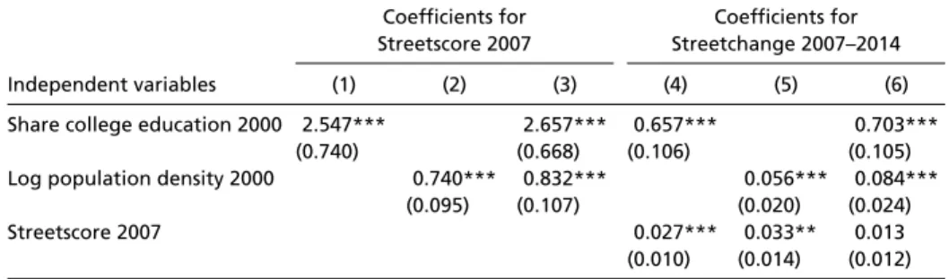
Table 2. Relationship between social characteristics and changes in Streetscore
Coefficients for Coefficients for
Streetscore 2007 Streetchange 2007–2014
Independent variables (1) (2) (3) (4) (5) (6)
Share college education 2000 2.547*** 2.657*** 0.657*** 0.703***
(0.740) (0.668) (0.106) (0.105)
Log population density 2000 0.740*** 0.832*** 0.056*** 0.084***
(0.095) (0.107) (0.020) (0.024)
Streetscore 2007 0.027*** 0.033** 0.013
(0.010) (0.014) (0.012)
All models control for city fixed effects.***P < 0.01,**P < 0.05.
total square footage corresponds to roughly half an SD increase
in Streetchange (seeSI Appendixfor details).
To relate the Streetscore indicators of neighborhood appear-ance to socioeconomic composition, we aggregated the Street-score and Streetchange variables at the census-tract level and obtained tract characteristic data from the 2000 US Census, adjusted to the 2010 census-tract boundaries (31). For summary statistics, see Table 1.
Results
We begin by presenting the cross-sectional demographic and economic correlates of cities’ physical appearances and changes in appearance, as estimated by 2007 Streetscore and Streetchange between 2007 and 2014 (Table 2). All regressions include city fixed effects and hold up in multivariate specifications. Addi-tionally, in all regressions we have corrected for spatial corre-lation in standard errors following Conley (32) using STATA routines developed by Hsiang (33). For each census tract we con-sider population density, level of education (share of college edu-cated adults), median income, housing price, rental costs, hous-ing vacancy, race, and poverty. From all of these variables the two strongest correlates of perception of safety are population density and education, so we present a table (Table 2) summarizing the coefficients of these two variables. (For a table with all controls seeSI Appendix, Table S4.)
Column 2 of Table 2 shows that Streetscores improve by 0.74 with the log of population density. This represents about one-quarter of an SD of Streetscore (2.6). Because Streetscores are
Fig. 2. Evidence of neighborhood tipping: We test the tipping model of neighborhood change. We group the data into 16 bins based on the initial value of Streetscore and plot the average Streetchange in each bin against the average initial Streetscore.
roughly linear in log density, the overall relationship is concave, meaning that perceived safety rises with density but the effect levels off. This fact lends some support to the idea that perceived safety increases with “eyes on the street” (34). However, our find-ing does not imply that dense urban spaces are seen as safer than low-density suburban or rural areas, because we do not have such low-density spaces in our sample. Our results suggest only that in five (generally dense) eastern US cities, spaces with high popula-tion densities are perceived as being safer than urban spaces with low population densities.
The second robust correlate of perceived safety is education (Table 2, column 1). As the share of the population with a col-lege degree increases by 20% (one SD), perceived safety rises by 0.51, or one-sixth of an SD in Streetscore. We suspect that the relationship reflects the tendency of educated people to be will-ing to pay for neighborhoods that appear safer, rather than the ability of educated residents to make a neighborhood feel safe.
We now move to changes in physical appearance—the primary contribution of this paper. Columns 4, 5, and 6 of Table 2 show the correlations between initial social characteristics, as mea-sured in the 2000 US Census, and neighborhood Streetchange as measured between 2007 and 2014.
Column 4 of Table 2 examines education, again controlling for initial Streetscore. The observed impact of education on Streetchange seems to be large. A one-SD increase in share with college degree in 2000 (20%) is associated with an increase in Streetchange of 0.13, or about one-sixth of an SD. Just as skilled cities have done particularly well over the last 50 y, skilled neigh-borhoods seem to have experienced more physical improvement. Column 5 of Table 2 shows that—controlling for initial Streetscore—as the log of density increases by 1 the growth in Streetscore increases by 0.06 points. The estimated impact of log
Table 3. Evidence of invasion
Coefficients for Streetchange 2007–2014
Independent variables (1) (2) (3) (4) Distance to CBD −0.042***−0.050***−0.051***−0.036*** (0.011) (0.011) (0.011) (0.011) Adjacent Streetscore 0.063*** 0.049** 2007 (0.019) (0.019)
Adjacent log population
density 2000 0.115** 0.093**
(0.046) (0.046)
Adjacent share college
education 2000 0.620*** 0.626***
(0.167) (0.172)
All models control for Streetscore 2007, Share college education 2000, and Log population density 2000 of a given census tract—along with city fixed effects.***
P < 0.01,**P < 0.05.
ECONOMIC SCIENCES
COMPUTER
SCIENCES
Fig. 3. The correlates of physical upgrading in neighborhoods: Positive urban change occurs in geographically and physically attractive areas with dense, highly educated populations, as illustrated here for Brooklyn, New York.
density on the Streetchange over a 7-y period is about 1/12 of the impact of log density on the level of Streetscore in 2007. Den-sity does seem to predict growth in Streetscore over the sam-ple period, but the relationship is far weaker than the connec-tion between density and the level of Streetscore in 2007. We did not find any robust relationships between Streetchange and median income, housing price, or rental costs; this suggests that the education effect is more likely to reflect skills than income (SI Appendix, Table S4).
The finding that variables that predict the level of Streetscore in 2007 also predict the change in Streetscore between 2007 and 2014 seems to support a positive feedback loop—the essence of tipping models (1, 2). Tipping is also suggested by the positive
correlation between 2007 Streetscore and Streetchange.‡
How-ever, we find a linear relationship, rather than the nonlinear rela-tionship suggested by the original tipping theory (2). Moreover, tipping models suggest that initially unattractive neighborhoods get worse over time—and that is not found in our data. The mean Streetchange by decile of 2007 Streetscore is positive even for the areas with the lowest scores (Fig. 2). It is not clear whether this represents tipping or a pattern in which visually safer areas are being upgraded first and faster. We suspect that the lack of downward movement may be particular to the time period under consideration. Despite the Great Recession, 2007–2014 was a relatively good time period for many of America’s eastern cities, and this may explain why we do not see declines even for less-attractive neighborhoods. Still, the data do show the overall pattern predicted by tipping models, in which upward growth is faster in initially better areas.
Next, we test for invasion (7) by regressing changes in Streetscore on characteristics of bordering neighborhoods and proximity to the CBD, after controlling for the predictors
identi-fied in Table 2 (2007 Streetscore, log of density, and education).§
The invasion hypothesis is just one of the reasons why areas may improve more when they have attractive neighbors—perhaps the most natural explanation is just that areas that are worse or bet-ter than their neighbors tend to mean-revert to the norm for their sections of the city. We test for the importance of loca-tion within the city by looking at the impact of proximity to the CBD. Column 1 of Table 3 shows that as the distance to the
‡Without the other controls, for each extra point of Streetscore in 2007, Streetscore
growth is 0.04 points higher over the next 7 y.
§CBD locations were based on the coding of Cortright and Mahmoudi (35).
CBD increases by 1 mile expected Streetscore growth falls by 0.04 points. Appearance upgrading is strongest closer to the city center, paralleling Kolko’s (36) finding that economic gentrifica-tion is more pronounced closer to the city center.
The original invasion hypothesis postulated a process under which low-income areas would gradually make their ways out from the center to nearby suburbs. The current pattern is instead one in which the central city sees particularly large upgrades in perceived street safety. One interpretation is that we are cur-rently witnessing the reversal of the process described by Burgess (7): City centers, which have always had a strong fundamental asset—proximity to jobs—are experiencing physical change that expresses a reversion to that fundamental.
Although the data do not suggest decay emanating out from a center, the core idea of the invasion hypothesis—that neighbor-hoods spill over into each other—is readily confirmed in the data. Column 1 of Table 3 also shows the effect of average Streetscore in surrounding areas on Streetchange. Notably, the coefficient on neighboring scores is more than double the impact of the neigh-borhood’s own score, implying that almost 1/10 of the Streetscore difference between a neighborhood and its neighbors is elimi-nated over a 7-y period. Because most of the movement over the sample period is positive, the regression should be interpreted as meaning that growth is faster in areas with more attractive neighbors. This strong convergence is exactly the prediction of the invasion theory.
Column 2 of Table 3 examines the effect of adjacent den-sity. Because adjacent density is highly correlated with adjacent Streetscore, it is not surprising to see that there is also a robust correlation here, although the connection is not as strong as with adjacent Streetscores. Column 3 of Table 3 looks at average share of the population with college degrees in adjacent areas. The relationship is positive and robust. As the share increases by 20%, Streetscore increases by 0.12 points. This again corrob-orates the results of Kolko (36), who found that gentrification is faster in areas with more educated neighbors. These findings point to a process of neighborhood spillovers and convergence,
which are, in a sense, at the heart of the invasion hypothesis.¶
¶In our working paper (37) we also looked at the “filtering” hypothesis, which suggests
the importance of the age of the building stock: Areas should gradually decline until they are upgraded. To test the hypothesis that building age shapes streetscape change, we regressed Streetchange on the shares of the building stock (as of the year 2000) built during different decades, controlling for 2007 Streetscore, log of density, and education. We found at best limited support for the filtering hypothesis (SI Appendix, Table S5).
Fig. 3 illustrates the relationship between location, education, population density, and physical improvement in neighborhoods
from Brooklyn, New York. InSI Appendix, Figs. S9–S28we
pro-vide similar map visualizations for all cities in our dataset. Conclusion
For decades, scholars from the social sciences and the humani-ties have discussed the importance of urban appearance and the factors that may contribute to physical urban change. Here, we test theories of urban change using Streetchange, a metric for change in urban appearance obtained from street-level imagery with a computer vision algorithm.
The data show that population density and education in both neighborhoods and their surrounding areas robustly predict improvements in neighborhoods’ physical environments; other variables show less correlation. The results also show strong sup-port for the invasion hypothesis of neighborhood change (7), which emphasizes spillovers across neighborhoods.
Our work suggests several open questions for future work. Is the correlation between density and perceived safety true more
generally, or does it mean-revert after a certain point? Does tip-ping appear when we examine cities with static or declining lev-els of Streetscore? We hope that future research, enabled in our part by our dataset and methods, can help address these ques-tions and continue exploring the links between the physical city and the humans that reside there.
ACKNOWLEDGMENTS. We thank Gary Becker, J ¨orn Boehnke, Graeme
Campbell, Steven Durlauf, Ingrid Gould Ellen, James Evans, Jay Garlapati, Lars Hansen, John William Hatfield, James Heckman, John Eric Humphries, Jackelyn Hwang, Paul Kominers, Michael Luca, Mia Petkova, Priya Ramaswamy, Matthew Resseger, Robert Sampson, Scott Stern, Zak Stone, Erik Strand, and Nina Tobio for helpful comments. This work was sup-ported by the International Growth Center, the Alfred P. Sloan Foundation, and a Star Family Challenge grant (to N.N., S.D.K., and E.L.G.); National Science Foundation Grants CCF-1216095 and SES-1459912 (to S.D.K.), the Harvard Milton Fund, the Ng Fund of the Harvard Center of Mathe-matical Sciences and Applications, and the Human Capital and Economic Opportunity Working Group sponsored by the Institute for New Economic Thinking (S.D.K.); the Taubman Center for State and Local Government (E.L.G.); as well as the Google Living Labs Award and a gift from Facebook (to C.A.H.).
1. Schelling TC (1969) Models of segregation. Am Econ Rev 59:488–493. 2. Grodzins M (1957) Metropolitan segregation. Sci Am 197:33–41.
3. Glaeser EL, Scheinkman JA, Shleifer A (1995) Economic growth in a cross-section of cities. J Monet Econ 36:117–143.
4. Bettencourt LM (2013) The origins of scaling in cities. Science 340:1438–1441. 5. Ciccone A, Hall RE (1996) Productivity and the density of economic activity. Am Econ
Rev 86:54–70.
6. Glaeser EL, Gottlieb JD (2009) The wealth of cities: Agglomeration economies and spatial equilibrium in the United States. J Econ Lit 47:983–1028.
7. Burgess EW (1925) The Growth of the City (Univ of Chicago Press, Chicago). 8. Lynch K (1960) The Image of the City (MIT Press, Cambridge, MA).
9. Rapoport A (1969) House Form and Culture (Prentice Hall, Englewood Cliffs, NJ). 10. Nasar JL (1998) The Evaluative Image of the City (Sage Publications, Thousand Oaks,
CA).
11. Milgram S (1976) Psychological maps of Paris. Environmental Psychology: People and
Their Physical Settings, eds Proshansky HM, Ittelson WH, Rivlin LG (Holt, Rinehart and
Winston, New York), pp 104–124.
12. Anguelov D, et al. (2010) Google street view: Capturing the world at street level. IEEE
Comput 43:32–38.
13. Rundle AG, Bader MD, Richards CA, Neckerman KM, Teitler JO (2011) Using Google street view to audit neighborhood environments. Am J Prev Med 40: 94–100.
14. Hwang J, Sampson RJ (2014) Divergent pathways of gentrification: Racial inequality and the social order of renewal in Chicago neighborhoods. Am Sociol Rev 79:726–751. 15. Salesses P, Schechtner K, Hidalgo CA (2013) The collaborative image of the city:
Map-ping the inequality of urban perception. PLoS One 8:e68400. 16. LeCun Y, Bengio Y, Hinton G (2015) Deep learning. Nature 521:436–444.
17. Naik N, Philipoom J, Raskar R, Hidalgo CA (2014) Streetscore – Predicting the per-ceived safety of one million streetscapes. Proceedings of the 2014 IEEE Conference
on Computer Vision and Pattern Recognition Workshops (IEEE, Washington, DC), pp
793–799.
18. Ordonez V, Berg TL (2014) Learning high-level judgments of urban perception.
Com-puter Vision – ECCV 2014. Lecture Notes in ComCom-puter Science, eds Fleet D, Pajdla T,
Schiele B, Tuytelaars T (Springer, Cham, Switzerland), Vol 8694, pp 494–510. 19. Porzi L, Rota Bul `o S, Lepri B, Ricci E (2015) Predicting and understanding urban
per-ception with convolutional neural networks. Proceedings of the 23rd ACM
Interna-tional Conference on Multimedia (ACM, New York), pp 139–148.
20. Been V, Ellen IG, Gedal M, Glaeser EL, McCabe BJ (2016) Preserving history or restrict-ing development? The heterogeneous effects of historic districts on local housrestrict-ing markets in New York City. J Urban Econ 92:16–30.
21. Harvey C, Aultman-Hall L (2016) Measuring urban streetscapes for livability: A review of approaches. Prof Geogr 68:149–158.
22. De Nadai M, et al. (2016) Are safer looking neighborhoods more lively? A multimodal investigation into urban life. Proceedings of the 2016 ACM on Multimedia
Confer-ence (ACM, New York), pp 1127–1135.
23. Doersch C, Singh S, Gupta A, Sivic J, Efros AA (2015) What makes Paris look like Paris?
Commun ACM 58:103–110.
24. Zhou B, Liu L, Oliva A, Torralba A (2014) Recognizing city identity via attribute analysis of geo-tagged images. Computer Vision – ECCV 2014. Lecture Notes in Computer Science, eds Fleet D, Pajdla T, Schiele B, Tuytelaars T (Springer, Cham, Switzerland), Vol 8691, pp 519–534.
25. Arietta SM, Efros AA, Ramamoorthi R, Agrawala M (2014) City forensics: Using visual elements to predict non-visual city attributes. IEEE Trans Vis Comput Graph 20:2624– 2633.
26. Glaeser EL, Kominers SD, Luca M, Naik N (2016) Big data and big cities: The promises and limitations of improved measures of urban life. Econ Inq, 10.1111/ecin.12364. 27. Hoiem D, Efros AA, Hebert M (2008) Putting objects in perspective. Int J Comput Vis
80:3–15.
28. Oliva A, Torralba A (2001) Modeling the shape of the scene: A holistic representation of the spatial envelope. Int J Comput Vis 42:145–175.
29. Malik J, Belongie S, Leung T, Shi J (2001) Contour and texture analysis for image segmentation. Int J Comput Vis 43:7–27.
30. Sch ¨olkopf B, Smola AJ, Williamson RC, Bartlett PL (2000) New support vector algo-rithms. Neural Comput 12:1207–1245.
31. Logan JR, Xu Z, Stults BJ (2014) Interpolating US decennial census tract data from as early as 1970 to 2010: A longitudinal tract database. Prof Geogr 66:412–420. 32. Conley TG (2008) Spatial econometrics. The New Palgrave Dictionary of Economics,
eds Durlauf SN, Blume LE (Palgrave Macmillan, New York).
33. Hsiang SM (2010) Temperatures and cyclones strongly associated with economic pro-duction in the Caribbean and Central America. Proc Natl Acad Sci USA 107:15367– 15372.
34. Jacobs J (1961) The Death and Life of Great American Cities (Vintage, New York). 35. Cortright J, Mahmoudi D (2014) Neighborhood change, 1970 to 2010: Transition and
growth in urban high poverty neighborhoods (Impresa Consulting, Portland, OR).
36. Kolko J (2010) The determinants of gentrification. Available at https://papers.ssrn. com/sol3/papers.cfm?abstract id=985714.
37. Naik N, Kominers SD, Raskar R, Glaeser EL, Hidalgo CA (2015) Do people shape cities,
or do cities shape people? The co-evolution of physical, social, and economic change in five major US cities. NBER Working Paper 21620 (National Bureau of Economic
Research, Cambridge, MA).