Complex Rotational Modulation of Rapidly
Rotating M Stars Observed with TESS
The MIT Faculty has made this article openly available. Please share
how this access benefits you. Your story matters.
Citation
Zhan, Z., et al. “Complex Rotational Modulation of Rapidly Rotating
M Stars Observed with TESS.” The Astrophysical Journal 876, 2 (May
2019): 127. © 2019 The American Astronomical Society
As Published
http://dx.doi.org/10.3847/1538-4357/AB158C
Publisher
American Astronomical Society
Version
Final published version
Citable link
https://hdl.handle.net/1721.1/124715
Terms of Use
Article is made available in accordance with the publisher's
policy and may be subject to US copyright law. Please refer to the
publisher's site for terms of use.
Complex Rotational Modulation of Rapidly Rotating M Stars Observed with
TESS
Z. Zhan1 , M. N. Günther2,14 , S. Rappaport2 , K. Oláh3 , A. Mann4 , A. M. Levine2 , J. Winn5 , F. Dai2,5 , G. Zhou6,15 , Chelsea X. Huang2,14 , L. G. Bouma5 , M. J. Ireland7 , G. Ricker2 , R. Vanderspek2 , D. Latham6 , S. Seager1,2,8 , J. Jenkins9 , D. A. Caldwell10 , J. P. Doty11, Z. Essack1 , G. Furesz2, M. E. R. Leidos9 , P. Rowden12 ,
J. C. Smith9,10 , K. G. Stassun13 , and M. Vezie2
1
Department of Earth, Atmospheric, and Planetary Sciences, MIT, Cambridge, MA 02139, USA;[email protected] 2
Department of Physics and Kavli Institute for Astrophysics and Space Research, MIT, Cambridge, MA 02139, USA 3
Konkoly Observatory, Research Centre for Astronomy and Earth Sciences, HAS, H-1121 Budapest, Konkoly Thege M.u. 15-17, Hungary 4
Department of Physics and Astronomy, University of North Carolina at Chapel Hill, Chapel Hill, NC 27599, USA 5
Department of Astrophysical Sciences, Princeton University, Princeton, NJ 08544, USA 6
Center for Astrophysics| Harvard & Smithsonian, 60 Garden Street, Cambridge, MA 02138, USA 7
Research School of Astronomy and Astrophysics, Australian National University, Canberra, ACT 2611, Australia 8
Department of Aeronautical and Astronautical Engineering, MIT, Cambridge, MA 02139, USA 9
NASA Ames Research Center, Moffett Field, CA 94035, USA 10
SETI Institute, Mountain View, CA 94043, USA 11
Noqsi Aerospace Ltd, 15 Blanchard Avenue, Billerica, MA 01821, USA 12
School of Physical Sciences, The Open University, Milton Keynes MK7 6AA, UK 13
Department of Physics and Astronomy, Vanderbilt University, 6301 Stevenson Center Lane, Nashville, TN 37235, USA Received 2019 February 24; revised 2019 April 1; accepted 2019 April 1; published 2019 May 10
Abstract
We have searched for short periodicities in the light curves of stars with Teff cooler than 4000 K made from
2-minute cadence data obtained in Transiting Exoplanet Survey Satellite sectors 1 and 2. Herein we report the discovery of 10 rapidly rotating M dwarfs with highly structured rotational modulation patterns among 371 M dwarfs found to have rotation periods less than 1 day. Starspot models cannot explain the highly structured periodic variations that typically exhibit between 10 and 40 Fourier harmonics. A similar set of objects was previously reported following K2 observations of the Upper Scorpius association. We examine the possibility that the unusual structured light curves could stem from absorption by charged dust particles that are trapped in or near the stellar magnetosphere. We also briefly explore the possibilities that the sharp structured features in the light curves are produced by extinction by coronal gas, by beaming of the radiation emitted from the stellar surface, or by occultations of spots by a dusty ring that surrounds the star. The last is perhaps the most promising of these scenarios. Most of the structured rotators displayflaring activity, and we investigate changes in the modulation pattern following the largestflares. As part of this study, we also report the discovery of 17 rapidly rotating M dwarfs with rotational periods below 4 hr, of which the shortest period is 1.63 hr.
Key words: circumstellar matter – stars: flare – stars: low-mass – stars: pre-main sequence – stars: variables: general – starspots
1. Introduction
Young M stars often are found to rotate rapidly, i.e., with periods2 days, and then are seen to be “active” in a number of different respects. The spectra of such stars may contain hydrogen and Ca H and K emission lines (Pettersen & Hawely 1989), flares on such stars are common (e.g.,
Davenport et al. 2019; Günther et al. 2019; Mondrik et al.
2019), and the stellar surfaces often have spots that result in
large-amplitude rotational modulations (e.g., EY Dra, Vida et al.2010; GJ 65A and 65B, Barnes et al.2017). Even though
the spots may be distributed around the stellar surface, the rotational modulation patterns are usually fairly simple, i.e., they may be adequately represented by just a few Fourier components. A small percentage of rotationally modulated stars, e.g., KIC 7740983(Rappaport et al.2014) and HSS 348
(Strassmeier et al. 2017), exhibit more complex rotational
modulations; even these can often be ascribed to particular sizes and arrangements of spots. Sometimes two distinct
rotation frequency signatures are seen, indicating the presence of two“twin-like” M stars (Rappaport et al.2014).
Two other quite distinct categories of young rotating M stars have recently been identified. First, there is a class of young late-type stars that exhibit “dipping activity” (see, e.g., Cody et al. 2014; Ansdell et al. 2016). Such stars can exhibit dips
with depths that range from∼5% to 50% and that may recur periodically, quasi-periodically, or without any apparent underlying pattern. These stars typically exhibit strong emission in the WISE 3 and 4 bands, indicating that dusty disks are present. Second, there is a class of stars found by Stauffer et al.(2017,2018) that may be related to the dippers,
which the authors describe as“rapidly rotating weak-line T Tau stars with orbiting clouds of material at the Keplerian co-rotation radius.” These stars were found in the Upper Scorpius and ρ Oph star-forming associations and exhibit highly structured rotational modulations that, according to the authors, cannot be explained by starspots.
In this work we present the discovery with the Transiting Exoplanet Survey Satellite (TESS; Ricker et al. 2015) of 10
rapidly rotating M stars in the southern hemisphere with quite complex rotational modulation patterns (the “10 complex rotators”). Half of these stars are in the star-forming stellar
© 2019. The American Astronomical Society. All rights reserved.
14
Juan Carlos Torres Fellow. 15
association Tucana Horologium (“THA”). In Section 2 we discuss the data from Sectors 1 and 2 that we searched for interesting rapid rotators. In Section3 we describe the Fourier transform survey of all the 2-minute cadence targets in Sectors 1 and 2 and discuss the Fourier amplitude spectra, the rotational modulation patterns, and other characteristics of the 10 complex rotators. Low- and medium-resolution spectra of a sample of the stars are presented in Section 4. We attempt to model the light curves with a starspot modeling code in Section 5, but we conclude that such a model falls short of explaining the observations. In Section 6 we discuss another model involving charged dust particles trapped in the stellar magnetosphere, but we find that this scenario also has difficulties. A model—perhaps the most promising one considered here—that involves a spotted host star rotating obliquely inside a dusty ring is presented in Section 7. In Section 8 we raise the possibility that the highly structured rotational modulations might be due to beamed emission. Changes in the structured modulation pattern around the time of a superflare in one of the rapid rotators are discussed in Section 9. In Section 10 we discuss the stellar associations where these 10 stars are found and their likely ages. We summarize our work and discuss some related issues in Section 11.
2. TESS Observations
In this study we utilized the 2-minute cadence (short-cadence) data collected by TESS during Sectors 1 and 2. The targets selected for short cadence are chosen from the candidate target list (CTL; Stassun et al. 2018). The light curves were
produced by the Science Processing Operations Center(SPOC) pipeline(Jenkins et al.2016), which is operated by the NASA
Ames Research Center, and are available online.16For Sectors 1 and 2, 2-minute cadence data were obtained for a total of 24,809 unique targets, of which 7074 were observed in both sectors. Although the primary goal of TESS is to search for terrestrial planets that transit nearby bright stars, the large number of targets monitored with 2-minute cadence enables the study of other astrophysical phenomena on timescales down to the Nyquist limit of 360 cycles day−1(4-minute period).
We opted to use the SAP_FLUX light-curve data and do our own detrending. For each light curve, we split the nonde-trended SAP_FLUX time series into separate orbits and then normalized the data for each orbit by the mean flux of that orbit. Since we were primarily interested in finding rapidly rotating M dwarfs, we detrended each orbit using a 3-day spline filter to remove any longer-timescale fluctuations in the flux.
We note that many of the M dwarfs in this study were added to the CTL as a part of the Cool Dwarf specially curated catalog(Muirhead et al.2018).
3. Analysis 3.1. Fourier Analysis
We used a basic fast Fourier transform (FFT) method to search for rapidly rotating M dwarf stars. The FFT method is fast and efficient when used to search for periodic signals that have high-duty cycles, or, equivalently, smoothly varying rotation profiles. The FFT search used here is similar to the one employed by Sanchis-Ojeda et al. (2013, 2014) but is
optimized for the TESS data. Given that the data set essentially consists of samples uniformly spaced in time and minimally affected by window functions, we did not see that any particular advantage would be gained by using the Lomb-Scargle transform (Lomb 1976; Scargle 1982). Accurate
periods and the corresponding uncertainties for any interesting objects are found via a Stellingwerf transform (Stelling-werf 1978) that utilizes a phase dispersion minimization
algorithm.
The preprocessed data for each orbit are stitched together into one data array, the mean flux is subtracted, and the data gaps are filled with zeros. The data array was extended by padding with zeros to a power of 2 number of bins, which represents approximately eight times the length of the nonzero part of the data array. This yields Fourier “interpolation” in frequency. In the case where only one TESS sector (two satellite orbits) of data (∼20,000 data points) is available, the final data array comprises 217bins. We then compute the FFT
using Python with the SciPy FFT package, which takes≈0.1 s for each object on a computer with a 2.9 GHz Intel Core i7 Processor. From the complex FFT we form the amplitude spectrum.
We apply the data preparation and Fourier transform operations to the data for all of the 2-minute cadence target stars. However, in this paper we focus on the results of our search for rapidly rotating M stars.
3.2. Finding Rapidly Rotating M Stars
To find rapidly rotating M dwarfs, we first select all stars among the 2-minute cadence targets with reported stellar temperatures Teff4000 K. Rapidly rotating M dwarfs are
known to be activeflaring stars; flares can add significant noise to the Fourier transform and thereby adversely affect the search (see Section 3). Therefore, flares are removed prior to
application of the FFT using a 5σ flare detection threshold andflare fitting technique developed and discussed in Günther et al.(2019).
To detect rapidly rotating M dwarfs, we compute a local, i.e., 128 frequency bin, mean and local rms(σ) for each bin in each Fourier amplitude spectrum. We consider a detection to be significant if at least one value in the amplitude spectrum exceeds the local mean by at least 5 localσ anywhere in the frequency range17of 1–48 cycles day−1and is accompanied by at least one higher harmonic or subharmonic that exceeds its local mean by 3 local σ. We vetted the targets that pass this threshold by eye to confirm detection and, in the process, eliminated eclipsing M star binaries and objects with other obvious nonrotational signals. The result was the detection of approximately 500 potentially rapidly rotating M dwarfs with periods shorter than 1 day in either one or both sectors, which accounts for roughly 1/10 of the M dwarf stars in the CTL for Sectors 1 and 2.
3.3. The Collection of Rapidly Rotating M Stars We found a total of 17 M dwarf stars to be rotating with periods less than 4 hr among 371 M dwarfs with periods below
16
http://archive.stsci.edu/tess/bulk_downloads.html
17
As noted earlier, the TESS short-cadence frequency range reaches 360 cycles day−1; however, we truncated our search at 48 cycles day−1 because even an M star of mass 0.1 Meand radius 0.15 Recannot rotate with a period
below 1/2 hr without breaking up owing to centrifugal forces (see discussion in Section3.3and Equation(1)).
2
1 day and∼1000 with periods below 2 days. With a period of 1.63 hr, TIC 204294226 is the most rapidly rotating M dwarf discovered thus far.
The 17 fastest rotators are listed in Table 1, along with coordinates and effective temperatures. The ratio of rotation frequency to breakup angular frequency is also listed for each star. The estimated breakup frequency of each star is based on the stellar mass, M*, and radius, R*, expressed as simple functions of the absolute K magnitude, MK, following Mann
et al.(2015,2019): R M M M a bM cM dM eM fM 1.9515 0.3520 0.01680 log , 1 K K K K K K K 2 10 2 3 4 5 * * - + + ¢ + ¢ + ¢ + ¢ + ¢ ( ) ( )
where MK¢ º MK -7.5 and the coefficients a−f are a=−0.642, b=−0.208, c=−0.000843, d=0.00787, e=0.000142, and f=−0.000213. The ratio of Ω/Ωcrit is
computed from the expression
P R GM r m P 2 2.8 hr , 2 crit 3 3 * * * * * * p W W = ⎛ ⎝ ⎜ ⎞⎠⎟ ( ) where m* and r* are the mass and radius in solar units, respectively, and P*is the rotational period in hours.
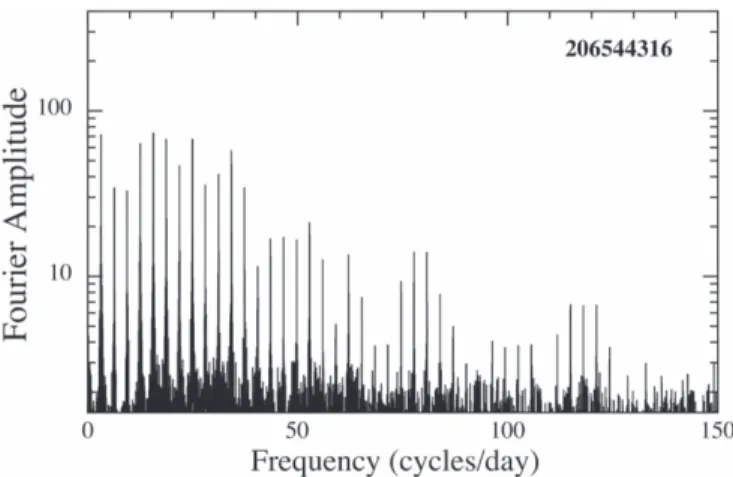
3.4. Identifying Highly Structured Rotation Profiles In the process of vetting the rapidly rotating M stars, we discovered a number of stars with highly structured rotational modulation patterns. The first clue came from examining the unusual harmonic structure in their amplitude spectra. An extreme example of this is shown in Figure 1. While the amplitude spectrum of a rotating M star usually contains two to
four detectable harmonics, TIC 206544316 exhibits 40 higher harmonics. This is indicative of a highly structured rotation profile.
The raw light curves for four of these objects are shown, as examples, in Figure 2. Note that each of these has a sharp structure that occurs over small fractions of a rotation cycle.
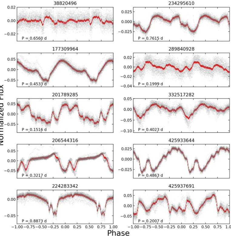
In all, wefind 10 similarly structured rotation curves among our sample of rapid rotators. Each of these objects exhibits 10–40 significant harmonics in the frequency range 1–96 cycles day–1. These contrast with most rapidly rotating M dwarfs that have comparatively simple modulation patterns and therefore exhibit only one to five significant harmonics. The folded light curves for these 10 rotators with complex modulation patterns are presented in Figure 3, and some of their properties are presented in Table2.
Table 1
M Stars with Rotation Periods P<4 hr in TESS Sectors 1 and 2
TIC R.A. J2000 Decl. J2000 Perioda(hr) T
effbK Ω/Ωcritc MKd Sectorse
204294226 345.3914 −22.0765 1.631(2) 3383 0.572 6.864 2 332507607 350.5944 −26.7901 2.100(1) 2877 0.332 7.719 2 261089844 81.5581 −83.6062 2.151(1) 3705 L L 1 231838187 24.9002 −64.9294 2.306(1) 2830 0.275 7.99 1, 2 120522722 2.8139 −37.9487 2.409(1) 2771 0.273 7.891 2 12419331 2.0585 −24.2320 3.149(1) 3336 0.320 6.627 2 300741820 115.1874 −66.8087 3.168(1) 2996 L L 1, 2 272466980 120.4676 −74.1727 3.318(1) 3143 0.397 5.802 2 389051009 333.4603 −63.7028 3.436(1) 2885 0.120 9.228 1 453095489 113.9139 −67.6945 3.699(1) 3299 0.285 6.488 1, 2 158596311 22.1261 −49.3526 3.711(1) 3096 0.281 6.525 2 441055710 359.4175 −15.8517 3.722(1) 2782 0.140 8.541 2 220478846 75.8890 −56.5118 3.827(1) 3665 0.410 5.267 1, 2 350296377 83.6215 −54.2042 3.833(2) 3410 0.274 6.507 1 314888837 50.9265 −81.8043 3.920(1) 2996 0.149 8.214 1 31381302 88.3600 −71.5638 3.965(1) 2871 0.109 9.069 1, 2 206502540 15.8985 −55.2656 3.998(1) 2898 L L 2 Notes. a
Error bars in parentheses are in the last digit, and error bars in the next digit are rounded to 1. b
The stellar temperature for each star is from TIC version 7(Stassun et al.2018) and was obtained via the Mikulski Archive for Space Telescopes (MAST) online portal.
c
The masses and radii required to evaluate the fractional breakup rotation frequency are obtained from the absolute K magnitudes and Equation(1). d
The absolute K magnitude is obtained from VizieR(http://vizier.u-strasbg.fr/; UCAC4 Zacharias et al.2013) and the Gaia distance (Lindegren et al.2018). Gaia parallaxes are not available for three of the objects.
e
Sector 1 spans BJD–2,457,000 from 1325 to 1353, while Sector 2 covers 1354–1382.
Figure 1.Fourier transform of the Sector 2 TESS data for TIC 206544316. The frequencies corresponding to the rotation period of 7.7274 hr and more than 40 detectable harmonics are evident, indicating that there is considerable high-frequency structure in the light curve down to timescales of∼4 minutes.
We see in Figure3an array of exotic rotational modulation patterns. To the extent we can generalize, the amplitudes of the modulations are typically 5%–10% peak to peak. The amplitudes and structures of the profiles seem roughly independent of rotation period between 2.5 and 21 hr. The structures of the profiles are not simple to describe; the term “scalloped shell” (Stauffer et al.2017), while descriptive, does
only partial justice. “Highly structured,” “comprised of many Fourier components,” and “multi- and sharply peaked” further describe the profile shapes.
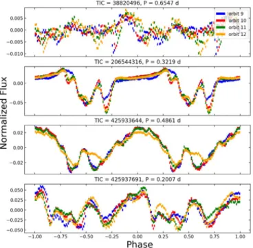
3.5. Variability of the Rotation Profiles over Time Figure 4 shows the light curves of four of our highly structured rotators for which data were obtained from both Sectors 1 and 2, i.e., from TESS orbits 9, 10, 11, and 12.18Each color-coded folded profile represents the data taken in one TESS orbit, i.e., 2 weeks. While there are clearly variations in the detailed shapes of the rotational modulations, the basic profiles remain recognizably similar over 2 months.
In Figure 5 we show the time evolution of the Fourier amplitude spectrum for TIC 332517282. For these calculations we used the software package TiFrAn (for details see Rappaport et al. 2014). Even though the amplitudes of some
of the features in the rotational modulation pattern are clearly changing with time, the fundamental frequency and its numerous harmonics remain essentially constant to within the frequency resolution over the course of a month.
3.6. Comparison with Highly Structured Rotators Found in Upper Sco andρ Oph
The rotational modulation profiles of the 10 M stars discussed in this work are very similar to those that Stauffer et al.(2017) describe as “scalloped shell” modulation profiles.
Of course, the 2-minute time resolution of the TESS data, when compared to the 30-minute resolution of the K2 data, allows for higher-frequency structure to be recorded. The “scalloped shell” rotators in Upper Sco and ρ Oph have a typical age of 5–10 Myr, a typical distance of 135 pc, and a median Ks
magnitude of 10.5 (median MK;4.9). The comparable
rotators in this work are ;45 pc away (closer), are ;45 Myr old (older), and have a similar median Ks magnitude but a
median MK;6.4, which is notably 1.5 mag less luminous than
the“scalloped shell” modulators in Upper Sco and ρ Oph. We also note that the range of periods of our 10 systems of 2.5–21 hr is comparable to the range of 6.2–15.4 hr of the “scalloped shell” modulators in Upper Sco and ρ Oph. Finally, we point out that the WISE W3fluxes of the stars in one set are similar to those of the other set, and the upper limits in the W4 band for the two sets of stars are similar.
4. Spectroscopic Observations
We obtained low- and medium-resolution spectra for a select sample of the rapidly rotating M dwarfs with complex rotational modulations to search for activity signatures and additional signs of rapid rotation. Low-resolution observations were obtained for four of the systems using the Wide Field Spectrograph(WiFeS; Dopita et al.2007) on the ANU 2.3 m
telescope at Siding Spring Observatory, Australia, on the nights of 2019 January 18 and 19. The data covered the wavelength region of 5200–7000 Å at a resolution of R≡λ/Δλ=7000 and were reduced per the procedure described in Bayliss et al. (2013). The spectra are displayed in Figure6. The spectra of all of the M dwarfs sampled by WiFeS exhibit strong Hα emission features with equivalent widths in the range of 4–6 Å, and none show signs of the composite nature expected if a system is composed of multiple stars. These Hα equivalent widths are quite typical of rapidly rotating M stars.
In addition to the low-resolution spectra from WiFeS, we also obtained a medium-resolution spectrum of TIC 206544316 using the echelle spectrograph on the ANU 2.3 m telescope. The echelle yields a spectral resolution of R=24000 over the wavelength region 4200–6725 Å, and the observations were reduced as per Zhou et al.(2014). The echelle spectrum of TIC
206544316 revealed that it is rapidly rotating at a rate of veqsin i∼77 km s−1, consistent with the equatorial rotational
velocity of the star derived from the photometric period. As with the WiFeS spectra, no obvious signatures of spectral blending indicative of multiple stars in the system are apparent. Wefind no evidence of ongoing accretion in these M dwarf systems. The Hα emission strengths as measured from our spectra are in line with that expected from rapidly rotatingfield M dwarfs(Newton et al.2017) and as such are not indicative of
accretion. It is difficult to quantitatively constrain the extent of veiling in our low-resolution spectra. We do not have accurate measurements of the rotational broadening, and as such it is more difficult to match the low-resolution spectra against synthetic templates while simultaneously fitting for line dilutions due to veiling. We suggest future observations at high resolution that may be able to address this problem.
Figure 2.Segments of raw data for four illustrative light curves of the rapid M star rotators we have found in the TESS Sectors 1 and 2 data that exhibit highly structured rotational modulations. Each plot shares the same time axis and is 1.4 days long.
18
Although there are data for TIC 177309964 from both sectors, they are not plotted because the modulation pattern is quite stable over the course of 2 months.
4
To further probe the spectra of our 10 highly structured rotators, especially in the near-IR (NIR), we utilized the observed spectral energy distribution (SED). We made use of photometric magnitudes from Gaia GBPand GRP(Brown et al.
2018); Two Micron All Sky Survey (2MASS) J, H, and Ks
bands (Cutri et al. 2003); and WISE W1, W2, W3, and W4
where available(Cutri et al.2013) to describe the SED of all 10
of our stars listed in Table2.
We compared the SEDs to a set of unreddened optical and NIR spectra from the TW Hydra or β Pic moving groups
(10–25 Myr; Bell et al. 2015), following the method from
Mann et al. (2016), which we briefly summarize here. We
restricted our comparison to templates with spectral types or Teffestimates consistent with the stars in Table2. Spectral types
and Teffvalues for the SED-fitting templates were determined
in an identical manner and hence were on the same overall scale. Gaps in the coverage of each template werefilled with PHOENIX BT-SETTL models (Allard et al. 2012). We
assumed zero reddening, as all targets are within the Local Bubble(Sfeir et al.1999).
Figure 3.Folded light curves for the 10 rapidly rotating M stars with complex rotational modulation profiles found in Sectors 1 and 2 with TESS. The fold periods are indicated. The red points are the folded and binned data, while the gray points are individualflux measurements (with flares removed). Almost all of the high-frequency features seen in the folds are statistically significant. The large fluctuations in the data for TIC 289840928 are due to the presence of another independent period at 15.606 hr. By contrast, the data for TIC 38820496 are intrinsically noisy.
Table 2
Rapidly Rotating M Stars with Complex Rotation Modulation Profiles
Object Name 38820496 177309964 201789285 206544316 224283342 234295610 289840928 332517282 425933644 425937691 R.A. J2000a 7.19516 103.45258 33.88868 18.41884 356.35758 357.98325 317.63150 350.87860 3.69942 5.36556 Decl. J2000a −67.86237 −75.70396 −56.45488 −59.65974 −40.33782 −64.79293 −27.18311 −28.12114 −60.06352 −63.85226 Teff(K)b 2987 3289 L 3112 3198 3082 3120 3032 3176 2733 d(pc)a 44.1±0.1 91.3±0.5 45.4±0.2 43.1±0.1 38.2±0.1 48.2±0.1 40.4±0.2 39.1±0.1 44.3±0.2 43.9±0.2 pmra(mas yr−1)a +89.2±0.1 +4.7±0.1 +95.3±0.1 +96.7±0.1 +108.4±0.1 74.6±0.1 +67.8±0.1 +109.3±0.1 +88.8±0.2 +91.6±0.2 pmdec(mas yr−1)a −50.9±0.1 39.3±0.1 −14.7±0.1 −41.0±0.1 −78.8±0.1 −59.7±0.1 −75.1±0.1 −123.5±0.1 −56.9±0.2 −53.9±0.2 Ga 14.77±[2] 14.45±[2] 15.63±[2] 12.95±[2] 13.66±[1] 13.89±[1] 13.60±[1] 14.74±[3] 12.71±[1] 14.76±[2] GBPa 16.80±0.01 16.13±0.01 18.04±0.01 14.61±[6] 15.42±[4] 15.65±[7] 15.56±[4] 16.70±0.02 14.31±[6] 17.12±0.02 GRPa 13.42±[4] 13.19±[6] 14.19±[5] 11.72±[5] 12.39±[2] 12.61±[4] 12.27±[2] 13.41±0.01 11.48±[3] 13.34±[7] Jc 11.40±0.03 11.36±0.03 11.93±0.02 9.95±0.02 10.53±0.02 10.72±0.026 10.30±0.02 11.41±002 9.71±0.02 11.02±0.02 Hc 10.77±0.02 10.73±0.03 11.32±0.03 9.34±0.03 9.95±0.02 10.17±0.024 9.71±0.03 10.83±003 9.10±0.02 10.48±0.03 Kc 10.5±0.02 10.48±0.03 10.95±0.02 9.06±0.03 9.69±0.02 9.88±0.021 9.41±0.02 10.51±0.02 8.83±0.02 10.11±0.03 MKa,c 7.278 5.680 7.666 5.888 6.784 6.464 6.379 7.545 5.602 6.896 W1d 10.31±0.02 10.35±0.02 10.66±0.02 8.90±0.02 9.50±0.02 9.71±0.022 9.06±0.02 10.32±0.02 8.70±0.02 9.91±0.02 W2d 10.09±0.02 10.15±0.02 10.40±0.02 8.71±0.02 9.30±002 9.51±0.019 8.81±0.02 10.13±0.02 8.51±0.02 9.66±0.02 W3d 9.95±0.05 10.00±0.04 10.16±0.05 8.58±0.02 9.13±0.03 9.27±0.034 8.77±0.03 9.90±0.05 8.36±0.02 9.40±0.03 W4d 8.65 9.35 8.5 8.46±0.26 8.5 8.46 8.41±0.33 8.5 8.17±0.25 8.5 Radius(Re)e 0.28±0.01 0.49±0.02 0.24±0.01 0.46±0.01 0.34±0.01 0.38±0.01 0.38±0.01 0.25±0.01 0.51±0.02 0.32±0.01 Mass(Me)e 0.25±0.01 0.49±0.02 0.18±0.01 0.35±0.01 0.25±0.01 0.37±0.01 0.29±0.01 0.19±0.01 0.38±0.01 0.30±0.01 Period(hr)f 15.727(6) 10.881(6) 3.638(1) 7.727(3) 21.298(11) 18.288(13) 4.780(3) 9.660(9) 11.669(6) 4.816(2)
Associationf THA CAR THA/CAR ABDMG COL THA BPMG ABDMG THA THA
Data sectorsg 1, 2 1, 2 2 1, 2 2 1 1 2 1, 2 1, 2
Notes.Error bars in parentheses are in the last digit, and error bars in square brackets are in the following digit.
a
Gaia DR2(Lindegren et al.2018).
b
TIC v.7(Stassun et al.2018).
c
2MASS catalog(Skrutskie et al.2006).
d
WISE point-source catalog(Cutri et al.2013).
e
See Equation(1); Mann et al. (2015,2019).
f
See Table3for more details; Gagné et al.(2018).
g
Sector 1 spans BJD–2,457,000 from 1325 to 1353, while Sector 2 covers 1354–1382.
6 The Astrophysical Journal, 876:127 (15pp ), 2019 May 10 Zhan et al.
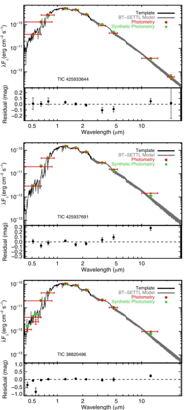
Afterfitting all 10 SEDs, we reach several conclusions: (1) Four of the SEDs show no NIR excess, e.g., TIC 206544316 and TIC 425933644 (see top panel of Figure 7) have W4
magnitudes, and both are in excellent agreement with the
model+template, and TIC 38820496 and TIC 177309964 are wellfit without any need for an excess. (2) Three of the systems show a clear NIR excess, e.g., TIC 425937691 (see middle panel of Figure7) and TIC 234295610 have W3 magnitudes
that are 4σ above the model, even considering the range of possible model fits, and TIC 201789285 is also a fairly clear case, with a possible W2 excess and a larger break at W3.(3) The remaining three systems fall in the ambiguous range, e.g., TIC 224283342 appears to show a W3 excess, but it is only barely significant. TIC 332517282ʼs W3 excess is not significant, just suggestive (see bottom panel of Figure7).
These results may be similar to what we would find if we were to randomly sample stars in these young stellar associations. However, the fact that some show clear excesses does lend credence to the notion that dust is involved. In particular, these excesses are consistent with what we would expect to see from a small dust disk near the star whose projected area is less than an order of magnitude larger than that of the host star, and having equilibrium grain temperatures of500 K (see Section7).
5. Modeling the Complex Light Curves with Spots 5.1. Fitting Stellar Spots withALLESFITTER
We studied whether the periodic variability of the 10 M stars may be explained by the presence of spots on the stellar surfaces. For this, we use theALLESFITTERpackage(Günther & Daylan 2019) to fit spot models of different complexities.
Using Nested Sampling(Skilling2006), we explore the entire
physical parameter space and compute the Bayesian evidence for different models.
Figure 4.Four examples of persistence of the rotational modulation patterns from TESS orbit to orbit. Orbits 9 and 10(color-coded blue and red) comprise TESS Sector 1 data, and similarly orbits 11 and 12(green and orange) comprise Sector 2 data.
Figure 5. Time-evolving Fourier amplitude spectrum for TIC 332517282 showing the stability of the modulation frequencies. The top panel shows the corresponding time series during Sector 2. The FWHM of the Gaussian window is 0.94 days, and the data are binned to 7.2 minutes, leading to a frequency resolution and Nyquist frequency of 1.1 and 200 cycles day−1, respectively. The Gaussian window is stepped by∼0.82 hr between Fourier transforms.
Figure 6.Low-resolution spectra for four of the rapidly rotating M dwarfs obtained with the ANU 2.3 m WiFeS facility. In each spectrum, we see strong Hα emission features at equivalent widths of 4–8 Å, indicative of strong chromospheric activity. We alsofind no evidence of binarity in any of the spectra. For comparability, each spectrum is normalized by the mean flux between 6000 and 6200Å.
ALLESFITTER19 is a publicly available, user-friendly soft-ware package built on the packages ELLC (light-curve and
radial velocity models; Maxted 2016), AFLARE (stellar flares;
Davenport et al.2014),DYNESTY(static and dynamic Nested
Sampling20), EMCEE (Markov chain Monte Carlo sampling;
Foreman-Mackey et al. 2013), and CELERITE (GP models;
Foreman-Mackey et al.2017).
We note two intrinsic approximations in the followingfits using ALLESFITTER. First, broadband photometric observa-tions, such as those represented by TESS light curves, do not allow us to discern any wavelength dependency of individual stellar surface features (e.g., warm plages vs. cool spots). Second, our approach describes a mean model, averaging over the lifetime and variability timescales of individual features (which can range from days to weeks).
5.2. Verification of Our Model on HSS 348
We verify our ability to fit spot models with ALLESFITTER
using the example of HSS 348, which shows one of the more complex spot configurations modeled in the literature (Strass-meier et al. 2017). HSS 348 is a B8+B8.5 double-lined
spectroscopic binary system. For comparison, we adopt the authors’ assumption that all spots are on one star. We mask out the eclipse region and phase-fold the CoRot data on the period reported in Strassmeier et al.(2017).
We ran two models, each containing four dark spots, on the phase-folded data. In the first model, the spin axis of the spotted star isfixed, according to the inclination of the binary system, which is known from eclipse observations to be normal to the binary orbital plane. The dilution is fixed to 50% to account for the light of the other star. We fit for 18 free parameters and adopt the following priors: four parameters for each of the four dark spots (longitude (0 , 360),21 latitude
90 , 90
- ( ), size (0 , 30), relative brightness (0, 1)), a linear limb-darkening term (0, 1), and the logarithm of a parameter for scaling the photometric error bars -( 8, 1) truncated to(−23, 0).22A small baseline offset taken to be the mean of the residuals is subtracted as part of each step in the sampling.
In the second model we keep the previous settings, except that we relax the assumption of afixed spin axis and fit for the additional parameter, the cosine (prior (0, 1)) of the angle between the axis of the spotted star and the plane of the sky.
Both spot models provide an excellentfit to the variability patterns of HSS 348. We compute the Bayesian evidence for each model in order to compare them quantitatively. Wefind significant Bayesian evidence for the model with the free spin axis. The best fit of the phase-folded profile and spot configuration for this model are shown in Figure8.
A casual comparison of our distribution of spots on the stellar surface with that of Strassmeier et al. (2017) indicates
some differences. This is not surprising, as those authors state that their spot solution is not mathematically unique. However, the difference lies basically in the fact that our modeling allows a different temperature for each spot while Strassmeier et al. (2017) assigned a temperature 1000K below that of the stellar
effective temperature to all four spots. A single spot in each quadrant of stellar longitude is sufficient to reproduce the light curve fairly well in both solutions, including the four observed minima. An advantage of using Nested Sampling is that it
λ λ
λ λ
λ
λ
Figure 7.SEDs of TIC 425933644, TIC 425937691, and TIC 332517282, with the optical defined by the Gaia GBPand GRPand the infrared defined by the
2MASS and WISE magnitudes. Observed magnitudes are shown in red, with vertical errors corresponding to the observed magnitude uncertainties (including stellar variability) and the horizontal errors corresponding to the width of thefilter. Synthetic magnitudes from the best-fit template spectrum (black) and BT-SETTL model (gray) are shown as green circles.
19
https://github.com/MNGuenther/allesfitter, online 2019 January 14.
20
https://github.com/joshspeagle/dynesty, online 2019 January 14, (Speagle2019).
21
A uniform probability distribution from a to b is denoted by(a b, ). 22
I.e., a normal distribution with a mean of−8 and standard deviation of 1, which is truncated to the range from−23 to 0.
8
allows one to search for multiple local and global maxima in the likelihood function. The solution shown in Figure 8 is in fact the only global likelihood maximum for our model.
5.3. Spots Alone Cannot Describe the Rapid Rotators Using models of two,five, or eight spots, which can here be either bright or dark, we try to describe the complex periodic variations of the rapid rotators using the ALLESFITTER code. We apply this to the light-curve data extracted by the SPOC pipeline. We do not apply any detrending procedure other than correcting for the dilution of known background stars. Each light curve is phase-folded on the prominent period identified for the respective object. We fit for the following parameters with priors: four parameters for each of the two,five, or eight spots (longitude (0 , 360), latitude - ( 90 , 90), size
0 , 30
( ), relative brightness(0, 2)), the cosine of the spin axis inclination (0, 1), a linear limb-darkening term(0, 1), and the logarithm of the parameter for scaling the photometric error bars -( 8, 1) truncated to(−23, 0). At each step in the sampling, the mean value of the residuals is computed and subtracted to remove any small baseline offset.
Figure 9 shows the results of the fit of eight spots to the rotational profile for TIC 201789285. The Bayesian evidence favors the eight-spot model over the two-spot and five-spot models. This is likely due to the fact that none of the models
yield an entirely adequatefit—the eight spots merely give the most freedom to“bend” the model curve to fit the sharp, high-frequency features. We note that the spot configuration shown in Figure9is locally nonphysical; in the model, overlying spots lead to a local stellar surface area with negativeflux.
In conclusion, even complex spot configurations cannot describe the sharp features found in the phase-folded light curves of these rapid rotators. While spots might contribute to the overall variability, additional physical effects close to the stars must be involved in the formation of the rotational profiles.
6. Magnetically Constrained Dust
Stauffer et al.(2017,2018) have suggested that the highly
structured rotational modulation patterns in their sample of Upper Sco andρ Oph stars are produced by “orbiting clouds of material at the Keplerian co-rotation radius.” Whatever produces the high-frequency structure in the phase-folded profiles of those stars is likely to also apply to the stars we report on in this work. Stauffer et al.(2017,2018) go on to say
that“we attribute their flux dips as most probably arising from eclipses of warm coronal gas clouds.” In this section we reexamine the possibility that absorption by dust rather than scattering by warm gas may be responsible for the dips.
Figure 8.A model of four spots on one star can describe nearly all of the periodic variability of HSS 348.ALLESFITTERwith Nested Sampling is used to compare different models. Wefind a single global likelihood maximum for the best-fit four-spot model. Left panel: phase-folded photometric data (blue error bars) and 20 posterior models(red curves). Right panel: best-fit spot configuration for one posterior sample.
Figure 9.A model comprising eight spots cannot adequately describe the periodic variability of TIC 201789285. While a simpler spot model can account for some overall trends, the sharp, high-frequency features of TIC 201789285 need to be explained by a different process.ALLESFITTERwith Nested Sampling was used to compare different spot models. Left panel: phase-folded photometric data(blue error bars) and 20 posterior models (red curves). Right panel: one posterior sample of the best-fit spot configuration. We note that this spot configuration is locally nonphysical, as overlying spots lead to a local stellar surface area that emits a negative flux. This stems from the model trying to replicate the sharp, non-spot-like features.
In order for dust to be the cause of the sharp rotational modulations, three requirements must be met:(1) there must be a sufficient amount of dust to account for the observed attenuation in flux, (2) the dust must be able to survive for at least days to weeks before sublimating, and (3) the dust must be located where it will corotate with the star, perhaps by virtue of being electrically charged and effectively locked onto magnetic field lines of the star (see, e.g., Farihi et al.2017).
Given that these stars are typically 40 Myr old, it is not obvious how much dust might remain close to each of them. A dust sheet comprising ∼1017g in submicron dust particles is required to block∼5%–10% of a star’s light.
Regarding the third point, the gyroradii of the charged dust particles must be much smaller than the orbital distance of the grains and no larger than the stellar radius. The radius of gyration is
R mv c
qB cgs , 3
g= ^ ( ) ( )
where m and q are the mass and charge of the dust grain, respectively, v⊥is the velocity perpendicular to the magnetic field of strength B, and c is the speed of light. If expressed as a ratio with respect to the stellar radius, the requirement becomes
R R c a Ne GM d d B R R R a N B P d R 4 3 2 1 0.06 1, 4 g s g 3 3 4 4 0.1 m 3 1000 1 3kG 1 crit,hr 1 5 2 * * * * * p r x x m - - - ⎛ ⎝ ⎜ ⎞⎠⎟ ( ) where, in the top equation, a is the grain radius, ρ is the bulk density of the grains, N is the number of electron charges on each grain, e is the electron charge, M*is the mass of the host star,ξ is v⊥in units of the freefall speed, Pcritis the rotational
breakup period of the host star, Bsis the surface magneticfield
(assumed dipolar), and d is the distance of the grain from the host star. In the bottom equation the expression has been evaluated for plausible values, e.g., the grain size in microns, number of charges per grain in units of 1000, Bs the surface
field in units of 3 kG, Pcritin units of hours,ξ normalized to 0.1,
and ρ is taken to be 3 g/cc. For the somewhat arbitrary normalizations used for these parameters, and for d/R*∼1 ( i.e., near the stellar surface), it is likely that the dust grains can be shepherded.
Regarding magneticfield strengths, the rapidly rotating and flaring M dwarf star V374 Peg is similar to the stars investigated in the present paper. Its rotational period is 0.4457 days=10.70 hr, while its mass and radius are 0.30 Me and 0.34 Re, respectively, all within the parameter ranges of the stars in Table2. V374 Peg has a low-amplitude stable light variation with some minor changes over time and has exhibited many flares, as well as a possible coronal mass ejection (see Vida et al. 2016for details). More importantly, this star may have a stable global poloidal magnetic field as modeled by Morin et al. (2008). The magnetic field of V374 Peg, in
locations, reaches strengths of 3–4 kG, implying an overall 1.5–2 kG field of the star (see Donati et al. 2006). New
measurements by Shulyak et al. (2017) reveal a 5.3±1kG
field on the star. Interestingly, the T Tauri star MN Lupi appears to have nearly the same rotation period, a large magneticfield of several kilogauss, and an active accretion disk
connected to the star via magneticfield lines (Strassmeier et al.
2005).
We next assess whether dust grains could survive for substantial times, e.g., a few days, close enough to the M stars that we are considering in this work. We do this in two steps by (1) computing the equilibrium dust grain temperatures, Teq, for
unshielded grains in circular orbits at each of a range of distances, i.e., orbital radii, from 1R* to 30R*, and(2) using Teqand the bulk properties of the grain material to compute the
sublimation time,τsub. We do this for grains of three different
sizes (0.1, 1, and 10 μm) and six different compositions revolving around a canonical M star with M*=0.3 Me, R*=0.4 Re, and Teff=3200 K. In order to compute Teq, we
solve the thermal balance equation by matching the emission of radiation at Teqto the absorption of radiation from the host star
at Teff (we ignore the cooling effects of sublimation, as this
effect is rarely important). To solve this equation, we utilize the grain absorption cross sections based on Mie scattering theory following Croll et al.(2014) and Xu et al. (2018). In turn, the
Mie calculations require, as input, the real and imaginary parts of the indices of refraction (n and k, respectively) of the dust grains(taken to be spherically shaped). We study six minerals that have been considered for the tails of the so-called “disintegrating exoplanets” (see, e.g., van Lieshout & Rappa-port 2018 for a review). These include iron (Querry 1985),
corundum(Begemann et al.1997), forsterite (Jäger et al.2003),
enstatite(Jäger et al.2003), and fayalite,23where the citations in parentheses are original sources of the corresponding n and k values. The sixth mineral is a generic “astronomical silicate” mixture (Draine1985). We obtained the indices of refraction
from the HITRAN aerosol database(Gordon et al. 2017) and
bulk mineral properties, such as the vapor pressure versusTeq,
from Table 5 of van Lieshout et al.(2016).
The results of this grain survival study are shown in Figure 10. The top panel shows the equilibrium grain temperatures as a function of distance from the host star out to 20R*; the corresponding Keplerian orbital periods are labeled along the top axis. For distances of5R*, the temperatures of the grains of iron, corundum, and fayalite (as well as cosmic silicates) are modestly high, while for forsterite and enstatite (the Mg-based silicates) the temperatures can be surprisingly low. This is due to the fact that these last two minerals have low values of k(∼0.001) near the wavelengths they are absorbing and relatively high values of k (∼1) at the much longer emission wavelengths. Grain sublimation times for 15 combinations of grain sizes and compositions that we consider are shown as a function of distance in the bottom panel of Figure 10. (Sublimation times for the astronomical silicate mixture are not given since there is no single set of mineral properties for this collection of materials.) We see that grains with sizes in a relevant range and composed of a number of kinds of minerals can survive for more than a day at distances of5R*, while grains of three offive mineral types can survive at distances of3R*; two offive can even survive relatively close to the stellar surface.
Perhaps the biggest difficulty with the dust grain model, or any other model invoking obscuration by intervening material (including coronal gas), lies in the distance from the host star where the material must be located. In order for any attenuating material to produce narrow duty-cycle features in the rotational
23
https://www.astro.uni-jena.de/Laboratory/Database/jpdoc/f-dbase.html
10
light curve, it must be situated considerably above the stellar surface. If f is the full width of the feature divided by the rotation period, the distance, d, from the stellar center, in units of the radius of the host star, R*, must be
dR*csc(pf). ( )5 If, for example, we consider narrow features with duty cycles, f, of 1%–10% (see, e.g., Figures 2–4), then d should be
3R*–30R*.(This is basically the reason that starspots with d/R*=1 do not work.) Such large factors of d/R* in Equation (4), raised to the 5/2 power, increase the leading
coefficient from 0.06 to values of ∼1–300, which quickly violates the requirement for meaningful constraint by the magnetic field.
7. A Dusty Ring Model
We now consider a model where the star is orbited by one or more rings composed of dust-size or somewhat larger particles. In this model, there would be no requirement for dust to be magnetically entrained in the stellar magneticfield at distances
of many stellar radii where the magnetic field would be relatively weak as in the magnetically constrained dust model discussed in Section 6. The ring particles would move in Keplerian orbits at relatively large distances from the star, and therefore the sublimation lifetime would not be an issue even if the particles are dust-like in size. Furthermore, there would be no requirement for small coherent dust structures to form and be maintained.
A sketch of the envisioned geometry is shown in Figure11. In terms of radial structure, either the disk could be mostly continuous with some gaps or thin regions, or it could comprise a small number of concentric rings. The ring(or rings) would be viewed at a tilt angle with respect to the edge-on orientation, ζ, which is small enough for the ring to partially occult the star. For a range of orientations of the star’s rotation axis such as that shown in thefigure, cool or warm spots will be hidden by the tilted rings for short time intervals as the star rotates and thereby produce rapid photometric changes.
Consider first just a single ring extending from radius r to r+Δr, or a gap in a more continuous ring of the same dimensions. We assume that the disk is thin, i.e., having a half-thickness h that satisfies h=Δr. With this configuration, there would be a nearly linear feature across the star of extra transmission or attenuation having a thickness ζΔr and a vertical displacement from the center of the star of ζr. A requirement for this gap to produce a sharp temporal feature as the star and its spots rotate beneath it is thatζΔr=R*. Afinal requirement is the existence of stellar surface features that can produce photometric modulations of order 1% by this mechanism. In turn, this implies the existence of regions with characteristic sizes where ~ D ~z r 0.1 *R and with surface brightnesses that are sufficiently different from the mean stellar surface brightness to produce∼1% effects.
Finally, in regard to a possible occulting ring, we can estimate a lower bound on its mass. The mass of a single uniform ring is given by
R R , 6
ring out2 in2
(p - )S ( )
where Rout and Rin are the outer and inner radii of the ring,
respectively, andΣ is the mass column density of the particles composing the ring in the direction normal to the ring plane. An illustrative set of parameters that could produce a sharp feature of width a few percent of the modulation period with ∼1% amplitude would be Rin=10R*, Rout=15R*,
R
0.2 *
= , and ζ=0.04;2°.
A ring consisting of micron-size dust particles with a projected number column density of∼1 μm−2would involve a minimum total mass to provide the desired light attenuation. In that case, for grains whose bulk material density is∼3 gm/cc,
Figure 10.Dust grain properties as a function of their distance in units of host star radius from a“standard” M star (see text). The corresponding Keplerian orbital periods are also indicated. Top panel: equilibrium temperature; bottom panel: sublimation lifetime. The color-coding legend describes the five minerals being considered; black on the top panel only indicates the “astronomical silicate” mixture of Draine (1985). Continuous, short-dashed, and long-dashed curves are for particle sizes of 0.1, 1, and 10μm, respectively. Dust grains composed of Mg-rich silicates(e.g., forsterite and enstatite) can survive for substantial periods quite close to the host star.
Figure 11. Sketch of a dusty ring geometry that might produce sharp modulation features. The disk plane is tilted by a small angleζ with respect to the edge-on orientation, and the stellar spin axis is oriented such that the stellar rotation will carry spots behind the disk for short time intervals. The radius of a stellar spot is denoted as .
the mass of a grain is ∼10−11 g, and Σ≈0.001 ζ g cm−2. Plugging this value for Σ, the above illustrative values of Rin,
Rout, andζ, and R*∼0.3 Reinto Equation(6), we find a mass
of≈1019g. The mass of the disk ring would be larger for larger particle sizes, Δr, or ζ.
Finally, we estimate the precession time for an inclined disk with the above parameters. We take the apsidal motion constant, k2, for the M stars to be that of an n=3/2 polytrope
with a value of k2;0.14 (Brooker & Olle 1955). From that,
we compute the J2 quadrupole term to be in the range of
0.001–0.024 for stellar rotation periods in the range of 1.6–4 hr. The resultant disk precession times are in the range of 10–70 yr, even for the shortest periods among the highly structured rotators.
8. Radiation Beaming
Beaming of the outgoing radiation is possibly another way of producing sharp features in rotational profiles. This could come about if radiation passing through magnetized plasma near the stellar surface has an anisotropic transmission factor.
Hamada & Kanno(1974) have computed how the Thomson
scattering cross section is modified in the presence of a strong magnetic field. For an unpolarized beam, incident at angle θ with respect to the magneticfield direction, the total scattering cross section is(Hamada & Kanno 1974)
u u u u
1 1 2 3 sin , 7
Th 2 2
s=s ( - )- [ + +( )( - ) q] ( )
where u is the ratioνC/νrad,νCis the cyclotron frequency,νrad
is the frequency of the radiation, and σTh is the classical
Thomson cross section. The cyclotron frequency is νC;3 BkGGHz, while the frequency of the radiation in the
TESS band is≈3×10¹⁴Hz. Since u is obviously quite small, we can expand Equation (7) in a Taylor series to show that
u
1 3 1 sin 2 . 8
Th 2
ss [ + ( - q ) ] ( )
Therefore, the magnitude of the difference in the cross section of radiation incident in the direction of the magnetic field versusperpendicular to it is of the order u∼10 ppm and therefore appears to be unable to lead to significant beaming.
Barring some other type of physical effect that can yield beaming that can, in turn, produce a ∼5% amplitude with beaming angles smaller than∼20°, we do not see how beaming can produce the effects we see.
9. Large Flares and Changes to the Rotational Modulation Pattern
The large flares that are sometimes observed in these stars may provide clues to the origin of the complex rotational modulation patterns. In fact, Stauffer et al.(2017,2018) found
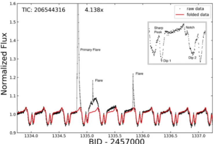
that the rotational modulation profile changed significantly afterflares were observed in some of the systems in Upper Sco. This prompted us to examine the behavior of our 10 rotators with structured modulation profiles after the occurrences of flares. In the TESS light curves, large flares where the intensity was seen to increase by more than a factor of two were observed on only 2 of our 10 stars, and of these, a distinct change in modulation profile was seen only in the light curve of TIC 206544316 after a large 4× superflare (Ebol=1.
7×1034erg; Günther et al.2019).
The light curve of this star around the time of this event is shown in Figure 12. In this figure the average 0.32-day
complex modulation pattern is shown in red, while the photometric measurements are shown in black. After the 4× flare, the three subsequent rotational profiles have larger amplitudes and somewhat different shapes. Two additional smallerflares erupt later, one during the next profile that has a strongly enhanced maximum brightness, and another three cycles later, again at higher maximum light than before or well after the bigflare.
About 25 rotations later than theflares shown in Figure12
another series of three or four flares with smaller peak brightnesses are observed within an interval offive rotations, and they occur at rotational phases similar to those seen in Figure12.
The two smaller flares seen in Figure 12 are likely “sympathetic flares,” that is, flares that sometimes appear, not merely by coincidence in time, soon after a large flare in analogy to such events that have been observed on the Sun(for the solar case see Török et al. 2011). Such temporally
correlated solar flares may be produced subsequent to disturbances of the large-scale magnetic field of the Sun from certain flares, as particular types of disturbances of the field may give rise later to other events at other locations on the Sun (see Schrijver & Title 2011). TIC206544316 has parameters
similar to those of V374Peg, which is inferred to have a strong and stable global magneticfield (see Section6). Thus, we can
suppose that there is a similar strong, global magneticfield on TIC206544316, which, after being disturbed, could induce additionalflaring events.
In light of the above, we interpret the disturbance to the light curve of TIC 206544316 in Figure 12 in the following way. First, we havefit the large flare by the same model discussed in Günther et al.(2019) and find it to be consistent with the flare
having decayed away by the time of the subsequent rotation of the host star. Second, the two prominent dips in the light curve are mostly unaffected by the flare for the next few rotations. However, another smaller feature (the “notch”), just after the maximum in the rotational profile, changes permanently after the flare. Third, we believe that the excess amplitude of the
Figure 12.Light curve of TIC 206544316 showing changes to the rotational modulation pattern following a large flare and around the times of two subsequent smaller flares. The black points are the normalized fluxes with 2-minute cadence. The overplotted red curve is the average rotational modulation pattern for this source. Substantial deviations from the mean profile are seen for three rotational cycles following the large flare. The inset panel shows a zoom-in on one of the modulation cycles that occurs well after the largeflare and is annotated to define various features discussed in the text.
12
profiles in the three rotations following the flare may be attributed to the aftermath of theflare.
Aside from this one dramatic event in TIC 206544316, we find no other case where a flare appears to be associated with a distinct change in either the shape or amplitude of the highly structured rotational profile of any of the other nine stars of our set.
In the dust model, a large flare could at least temporarily change the modulation profile of the star by, e.g., inducing changes in the configuration of the magnetic field, by increasing the rates at which grains sublimate, or by inducing changes in the amounts of net electrical charge on the grains. Likewise, in the model noted by Stauffer et al.(2017), which
invokes corotating coronal gas as a scattering mechanism, a largeflare may also be expected to result in temporary changes in the modulation profiles. Our observation of changes in the modulation profile of one star following one flare is not sufficient to give us insight into the physical mechanisms underlying the modulations and certainly on its own does not confirm or contradict any of the models we have considered.
10. The Stellar Associations
Rapidly rotating M dwarfs are often young and, conse-quently, close to the stellar associations into which they were born. In such cases, the stellar ages may be estimated from the ages of the stellar associations. To try tofigure out which stellar association each of our target stars might belong to, we used the online BANYANΣ Bayesian analysis tool relevant to nearby young associations (Gagné et al. 2018). If provided sufficient
information about the six-dimensional phase-space coordinates of a star(Table2), BANYAN Σ assesses the likelihood that the
star belongs to one of the 27 known and well-characterized young associations within 150 pc of the Sun.
Each of our 10 objects is most likely to be a member of the stellar association given in Table2. Five out of 10 belong to the association Tucana Horologium. For convenience, we give in Table3the names, distances, and ages of thefive associations listed in Table2. These associations all have distances between 30 and 50 pc, and the ages of four of thefive are between 25 and 50 Myr.
These ages of ∼40 Myr are considerably older than the nominal 10 Myr age of the Upper Scorpius association(Pecaut et al. 2012; Feiden 2016), which houses many of the known
dippers, as well as the structured rotators found by Stauffer et al.(2017,2018). It is not clear whether it is reasonable or not
to postulate that 40 Myr old M stars can accrete sufficient amounts of dust into their magnetospheres to produce the observed rotational modulations.
11. Summary and Discussion
In this work we have reported the discovery, using thefirst two sectors of TESS data, of 10 new rapidly rotating M dwarfs with highly structured rotational modulation patterns. The overall shapes of the periodic patterns can remain stable for weeks, while individual features can change within days. As part of this study, we also report the discovery of 17 rapidly rotating M dwarfs with periods <4 hr, of which the shortest period is 1.63 hr. These objects are part of a sample of 371 rapidly rotating M dwarfs also found in thefirst two sectors of TESS data with Teff cooler than 4000 K and with rotation
periods<1 day.
We attempt to better understand the nature of the rapidly rotating M dwarfs with highly structured rotational modulation patterns, which are similar in their properties to a number of stars found in the Upper Sco stellar association(Stauffer et al.
2017). First, we fitted general starspot models, able to
accommodate large numbers of spots, to these periodic variations, which exhibit large amounts of structure (Section5). However, we show that spots are not likely to be
able to explain the sharp features in the light curves(see also Stauffer et al.2017). Next, we explored the possibility that the
highly structured rotational modulation patterns are due to absorption by charged dust particles that are trapped by the stellar magnetosphere(see Section6). We have shown that dust
grains may be able to survive for a number of rotation periods in the magnetosphere at the corotation radius. However, such dust would have to be substantially far from the host star(see Equation (5)) to produce the sharp features observed in the
rotation profiles, and the existing magnetic fields at those distances would likely be too weak to trap charged dust particles (see Section 6). Beaming of the emitted radiation
would be a desirable mechanism, but we show, at least in the case of electron scattering in a magneticfield, that the observed amplitudes of a few percent are not achievable(Section8). We
did not explore the scenario, proposed by Stauffer et al.(2017),
involving attenuation by scattering from warm coronal material because it is difficult to conceive of a situation where it would produce significant emission or absorption.
Perhaps the most natural of the scenarios we have explored is that of a spotted host star rotating obliquely inside of a dusty ring of material a few tens of stellar radii away (Section 7).
While potentially very promising, this model has not been fully fleshed out, and a determination of whether it can quantitatively explain the sharp modulation structures that are observed will require further exploration. However, this is beyond the scope of the present work.
In addition, we explore whether largeflares could serve as probes of the highly structured rotational modulation patterns. We found 32 largeflaring events with flux increases larger than two times the stellarflux. However, we do not see any changes in the intrinsic rotational modulation pattern after mostflares. The exception is a large 4× superflare event (Ebol=1.7×1034erg) on TIC206544316, which is the
strongest flare observed to date in such a rapidly rotating M dwarf with highly structured rotational modulation patterns. This superflare apparently changes the subsequent periodic modulation by increasing the maximum brightness for a few rotations and altering one feature permanently.
Because most of our 10 highly structured rotators are in well-studied stellar associations, their ages are known reasonably well. Therefore, we are able to compare some of the properties
Table 3
Data from Gagné et al.(2018)
Name Abbr. Ave. Dist.(pc) Age(Myr)
AB Doradus ABDMG 30-+1020 149-+1951 β Pictoris βPMG 30 1020 -+ 24±3 Carina CAR 60±20 45-+711 Columba COL 50±20 42 46 -+
of our stars with the“scalloped shell” rotators in Upper Sco and ρ Oph. The latter have ages of 5–10 Myr, distances of about 135 pc, and a median Ks magnitude of 10.5 (median
MK;4.9). The comparable rotators in this work are some
three times closer and several times older. Both sets of stars have a similar median Ks magnitude but a median MK;6.4,
which is, perhaps not surprisingly, 1.5 mag less luminous than the “scalloped shell” modulators in upper Sco and ρ Oph, which are younger.
A small sample of low-mass stars revealing periodic optical variability has also been found to be radio active (see, e.g., Harding et al. 2013)—however, we note that their optical
modulations seem not as sharp featured as those of our rapid rotators. For these radio active low-mass stars, electron cyclotron maser emission is suggested to cause periodic, circularly polarized radio pulses (see, e.g., Hallinan et al.
2007). Notably, the ultracool dwarf TVLM 512-46546 shows
sharp radio bursts every 1.96 hr (Hallinan et al. 2007) and
smooth optical modulations with a similar ∼2 hr period (Littlefair et al. 2008; Harding et al. 2013). The latter was
attributed to inhomogeneous dust clouds in the relatively cool stellar atmosphere (Littlefair et al.2008). This short period is
remarkably similar to the periods of our 10 complex rotators and suggests that the optical and radio emission are linked by common magnetic phenomena. The modulation signal of TVLM 512-46546, for example, is stable over a time span of 5 yr. Neither spots nor magnetically constrained dust could explain such long-term stability. Whether the modulations of our targets are as long-lived may be studied in the future.
The mechanism that produces the observed highly structured rotational modulation patterns has not yet been confidently identified. In that regard, we have discussed, in Section 7, a promising idea. Continued observation of these 10 complex rotators will also provide opportunities to further understand the relevant physical processes. Ideally, this will encompass observations of time variability in the radio band, in both optical and NIR bandpasses, and in Hα; spectroscopy well beyond that presented in Section 4); and direct imaging.
Finding ∼100 more of these objects in the upcoming TESS sectors, as we anticipate, will hopefully further elucidate their nature.
This work was carried out as part of a larger search for rapid rotation and high-frequency oscillations in the TESS data. The methods described herein can also be applied to other high-frequency stellar phenomena.
The authors are grateful to the reviewer, Klaus Strassmeier, for a number of important suggestions that improved the manuscript. We acknowledge the use of public data collected by the TESS mission, which are from pipelines at the TESS Science Office and at the TESS Science Processing Operations Center and made publicly available from the Mikulski Archive for Space Telescopes (MAST). Funding for the TESS mission is provided by NASA’s Science Mission directorate. Resources supporting this work were provided by the NASA High-End Computing (HEC) Program through the NASA Advanced Supercomputing(NAS) Division at Ames Research Center for the production of the SPOC data products. M.N.G. acknowl-edges support from MIT’s Kavli Institute as a Torres postdoctoral fellow. We are grateful to Lidia van Driel-Gesztelyi for input about solar analogs to some of the observed features of the systems studied in this work.
Software:PYTHON (Rossum 1995), NUMPY (van der Walt
et al. 2011), SCIPY (Jones et al. 2001), MATPLOTLIB
(Hunter 2007), TQDM (doi:10.5281/zenodo.1468033), SEA-BORN (https://seaborn.pydata.org/index.html), ALLESFITTER
(Günther & Daylan 2019, in preparation),ELLC(Maxted2016),
AFLARE (Davenport et al. 2014), DYNESTY (Speagle 2019),
CORNER(Foreman-Mackey2016). ORCID iDs Z. Zhan https://orcid.org/0000-0002-4142-1800 M. N. Günther https://orcid.org/0000-0002-3164-9086 S. Rappaport https://orcid.org/0000-0003-3182-5569 K. Oláh https://orcid.org/0000-0003-3669-7201 A. Mann https://orcid.org/0000-0003-3654-1602 A. M. Levine https://orcid.org/0000-0001-8172-0453 J. Winn https://orcid.org/0000-0002-4265-047X F. Dai https://orcid.org/0000-0002-8958-0683 G. Zhou https://orcid.org/0000-0002-4891-3517
Chelsea X. Huang https://orcid.org/0000-0003-0918-7484
L. G. Bouma https://orcid.org/0000-0002-0514-5538 M. J. Ireland https://orcid.org/0000-0002-6194-043X G. Ricker https://orcid.org/0000-0003-2058-6662 R. Vanderspek https://orcid.org/0000-0001-6763-6562 D. Latham https://orcid.org/0000-0001-9911-7388 S. Seager https://orcid.org/0000-0002-6892-6948 J. Jenkins https://orcid.org/0000-0002-4715-9460 D. A. Caldwell https://orcid.org/0000-0003-1963-9616 Z. Essack https://orcid.org/0000-0002-2482-0180 M. E. R. Leidos https://orcid.org/0000-0003-4724-745X P. Rowden https://orcid.org/0000-0002-4829-7101 J. C. Smith https://orcid.org/0000-0002-6148-7903 K. G. Stassun https://orcid.org/0000-0002-3481-9052 References
Allard, F., Homeier, D., & Freytag, B. 2012,RSPTA,370, 2765 Ansdell, M., Gaidos, E., Rappaport, S., et al. 2016,ApJ,816, 69
Barnes, J. R., Jeffers, S. V., Haswell, C. A., et al. 2017,MNRAS,471, 811 Bayliss, D, Zhou, G., Penev, K, et al. 2013,AJ,146, 113
Begemann, B., Dorschner, J., Henning, Th., et al. 1997,ApJ,476, 199 Bell, C. P. M., Mamajek, E. E., & Naylor, T. 2015,MNRAS,454, 593 Brooker, R. A., & Olle, T. W. 1955,MNRAS,115, 101
Brown, A. G. A., Vallenari, A., Prusti, T., et al. 2018,A&A,616, A1 Cody, A. M., Stauffer, J., Baglin, A., et al. 2014,ApJ,147, 82 Croll, B, Rappaport, S., DeVore, J., et al. 2014,ApJ,786, 100
Cutri, R. M., Skrutskie, M. F., van Dyk, S., et al. 2003, The IRSA 2MASS All-Sky Point Source Catalog, NASA/IPAC Infrared Science Archive Cutri, R. M., Wright, E. L., Conrow, T., et al. 2013, Explanatory Supplement to
the AllWISE Data Release Products, wise.rept, 1C
Davenport, J. R. A., Covey, K. R., Clarke, R. W., et al. 2019,ApJ,871, 241 Davenport, J. R. A., Hawley, S. L., Hebb, L., et al. 2014,ApJ,797, 122 Donati, J.-F., Forveille, T., Collier Cameron, A., et al. 2006,Sci,311, 633 Dopita, M., Hart, J., McGregor, P., et al. 2007,Ap&SS,310, 255 Draine, B. T. 1985,ApJS,57, 587
Farihi, J., von Hippel, T., & Pringle, J. E. 2017,MNRAS,471, 145 Feiden, G. A. 2016,A&A,593, A99
Foreman-Mackey, D. 2016,JOSS,1, 24
Foreman-Mackey, D., Agol, E., Ambikasaran, S., & Angus, R. 2017, AJ, 154, 220
Foreman-Mackey, D., Hogg, D. W., Lang, D., & Goodman, J. 2013,PASP, 125, 306
Gagné, J., Mamajek, E. E., Malo, L., et al. 2018,ApJ,856, 23 Gordon, I. E., Rothman, L. S., Hill, C., et al. 2017,JQSRT,203, 3 Günther, M. N., & Daylan, T. 2019, Flexible Star and Exoplanet Inference
from Photometry and Radial Velocity Astrophysics Source Code Library, ascl:1903.003
Günther, M. N., Zhan, Z., Seager, S., et al. 2019, ApJ, arXiv:1901.00443 Hallinan, G., Bourke, S., Lane, C., et al. 2007,ApJ,663, L25
14