HAL Id: hal-01410206
https://hal.archives-ouvertes.fr/hal-01410206
Submitted on 16 May 2020
HAL is a multi-disciplinary open access
archive for the deposit and dissemination of sci-entific research documents, whether they are pub-lished or not. The documents may come from teaching and research institutions in France or abroad, or from public or private research centers.
L’archive ouverte pluridisciplinaire HAL, est destinée au dépôt et à la diffusion de documents scientifiques de niveau recherche, publiés ou non, émanant des établissements d’enseignement et de recherche français ou étrangers, des laboratoires publics ou privés.
Nicolas Forquet, Matthieu Dufresne
To cite this version:
Nicolas Forquet, Matthieu Dufresne. Simple deterministic model of the hydraulic buffer effect in septic tanks. Water and Environment Journal, Wiley, 2015, 29 (3), pp.360-364. �10.1111/wej.12114�. �hal-01410206�
Simple deterministic model of the hydraulic buffer effect in septic
1
tanks
2
Nicolas Forquet1 and Matthieu Dufresne2 3
Abstract
4
Septic tanks are widely used in on-site wastewater treatment systems. In addition to anaerobic pre-5
treatment, hydraulic buffering is one of the roles attributed to septic tanks. However there is still no 6
tool for assessing it, especially in dynamic conditions. For gravity fed-system, it could help both 7
researchers and system designers. This technical note reports a simple mechanistic model based on the 8
assumption of flow transition between the septic tank and the outflow pipe. The only parameter of this 9
model was calibrated using CFD modeling for a wide range of discharge rates. The resulting model 10
highlights that a septic tank plays a hydraulic buffer role when faced with sudden and large discharge 11
flow but this role tends to disappear when input hydrographs are smoother. In those cases there is an 12
observable lag between the input hydrograph and outflow hydrograph. 13
Key words: on-site wastewater treatment – septic tank – buffer effect – mechanistic modeling
14
Introduction
15
On-site wastewater systems usually consist of a septic tank followed by a treatment unit. In many 16
countries (including the USA and France), treatment units are commonly gravity-fed from the outlet of 17
the septic tank (e.g. a drainfield trench or vertical flow sand filter). Because flow at the outlet of a 18
septic tank is not constant, the distribution over the surface of the treatment unit is rather uneven, 19
especially in early filter operation (Bridson-Pateman et al., 2013; Gill et al., 2009). Flow variability 20
stems mainly from household water usage patterns, but the septic tank also induces some flow 21
modulation. The hydraulic buffer effect of septic tanks is often cited but to our knowledge there is still 22
no method for quantifying it. It is often assumed that for the purposes of studying of long-term 23
phenomena (like clogging of the treatment unit at month-long or year-long scale), the outflow can be 24
considered constant (Winstanley & Fowler, 2013). However, as we gain progressively more 25
knowledge on the actual hydrograph produced by a household, it may be interesting to quantify how 26
effectively the septic tank can buffer large inflow rates. This may be of particular interest for 27
estimating the efficiency of gravity-driven distribution on secondary treatment unit and to eventually 28
optimize it. 29
1 Irstea, UR MALY, centre de Lyon-Villeurbanne, 5 rue de la Doua – CS 70077, 69626 Villeurbanne Cedex,
France. [email protected]
2 Ecole Nationale du Génie de l'Eau et de l'Environnement de Strasbourg, Laboratoire ICube (Université de
Two possible approaches were identified: (i) using a tank model where the law governing outflow is 30
obtained by a statistical learning or neural network method (Vazquez et al., 1999) or (ii) the overflow 31
analogy. A statistical learning or neural network method is able to mimic complex hydraulic systems 32
without the need to compile advanced knowledge of the constitutive elements. However, it requires a 33
large dataset for model learning, which is not compatible with our needs. The overflow analogy is 34
based on a simple mechanistic approach based on the assumption that critical flow occurs at the outlet 35
of the septic tank. In this paper, we briefly present the model and its practical implementation, and 36
then report selected results based on several hydrographs. 37
Model presentation
38
Model equations
39
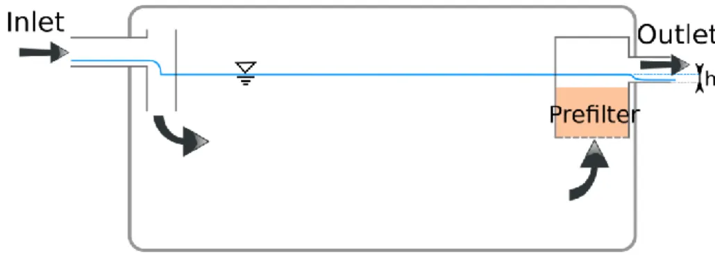
Figure 1 presents a sketch of the usual design of a septic tank. The upstream section of the outflow 40
pipe of a septic tank is a local maximum of the bottom profile. With no downstream influence 41
(guaranteed by the large slope of the pipe, which is usually over 0.5%; AFNOR, 2007), this 42
configuration is responsible for producing critical flow (Hager 1999). Critical flow is the transition 43
between subcritical flow (here, a nearly horizontal water surface with a very small velocity in the 44
septic tank) and supercritical flow (here, a fast flow in the outflow pipe). The occurrence of critical 45
flow guarantees a direct relationship between water level h in the tank and the outflow discharge (Qout
46
[L3T-1]). We used this relationship in association with a water mass balance in the septic tank to build 47
a time-dependent model. 48
49
Figure 1. Sketch of the water flow through a septic tank
50
The discharge Qout corresponding to the critical water depth hc [L] can be evaluated considering a
51
Froude number equal to unity (transition from subcritical to supercritical flow), according to: 52 hc c out
S
gD
Q
(1) 53where Qout is outflow discharge [L 3
T-1], Sc is critical cross-section [L 2
], g is gravitational acceleration 54
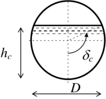
[L T-2] and Dhc is critical hydraulic diameter [L]. Both Sc and Dhc are linked to the critical water depth
55
(hc) by relationships (Equations 2, 3 and 4) using the angle δc as illustrated in Figure 2.
h
cD
c57
Figure 2. Relationships between critical water depth and hydraulic section and pipe diameter
58
c c c
cD
S
sin
cos
4
2
(2) 59
c c c c hcD
D
sin
4
cos
sin
(3) 60
c
cD
h
1
cos
2
(4) 61where D is outlet pipe diameter [L]. The angle δc may be expressed as a function of D and hc:
62
D
h
a
c ccos
1
2
(5) 63Equation 1 links the outflow discharge to the critical water depth in the outflow pipe. We are now 64
seeking out a relationship between critical water depth (hc) and the water depth in the tank (h [L],
65
measured from the invert of the outflow pipe). Knowing the critical water depth (hc), the critical
66
energy head Hc [L] can be calculated with the following expression.
67 2 2
2
c out c cgS
Q
h
H
(6) 68The head loss ΔH [L] between the tank and the critical section can be evaluated as a local head loss, 69 thus: 70 2 2
2
c outgS
Q
K
H
(7) 71The loss coefficient K [-] was evaluated by CFD using the OpenFOAM software package (2013) for a 72
100 mm diameter pipe and a flow rate ranging from 0.10 to 1.50 L/s. The conclusion of the numerical 73
simulations is that the loss coefficient K is approximately 0.4 for the whole discharge range. Using this 74
value and an estimation of the numerical uncertainty based on a grid sensitivity analysis, the 75
uncertainty on the outflow discharge (Qout) for a given water depth (h) was evaluated as 5%. Finally,
the water depth in the tank (h) can be evaluated using equation 7 (Bernoulli equation written between 77
the critical section and the tank where the velocity head is close to zero). 78
H
H
h
c
(8)79
Based on equations 6 and 7, equation 8 can be rewritten as: 80
2 22
1
c out cgS
Q
K
h
h
(9) 81Replacing hc and Sc in equation (9) by expressions dependent solely on Qout will lead to an expression
82
relating tank water depth (h) to outflow discharge (Qout). However, analytically solving this equation
83
would prove cumbersome due to the sinusoidal functions involved. An alternative solution was found 84
that consisted in rewriting equation 8 into a minimization problem. Incorporating equation (1) into 85 equation (9) implies: 86 hc c
D
K
h
h
2
1
(10) 87Rewriting equation 10 into the form of an objective function (obj.fun) gives: 88 2
2
1
)
(
.
c hc cD
K
h
h
h
fun
obj
(11) 89For a given value of h, finding the value of hc that minimizes the objective function makes it possible
90
to compute the outflow discharge (Qout) using equation 1. Once this relation has been established, it
91
can be associated to the septic tank mass balance equation to build a time-dependent model. For a 92
septic tank, the water mass balance can be written as: 93 out in
Q
Q
dt
dh
S
(12) 94where S is horizontal surface of the septic tank at the level of the invert of the outflow pipe [L2], and 95
Qin is inflow rate [L3T-1]. 96
After an explicit discretization, equation 12 becomes: 97
)
(
)
(
)
(
)
(
t
Q
t
Q
t
t
h
t
t
h
S
in
out
(13) 98The value of Qin(t) is an input while the value of Qout(t) needs to be estimated (except for the initial
99
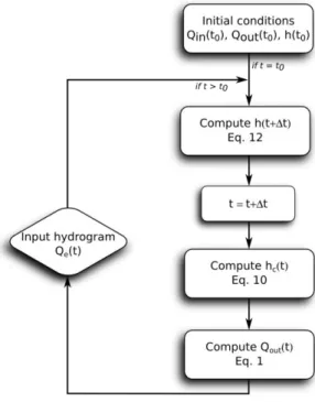
value). This is carried out by minimizing the objective function (11) at time t. Figure 3 schematizes the 100
basic computation steps. 101
102
Figure 3. Computation steps
103
Model implementation
104
The model was implemented in R (R Core Team, 2013). The method used for minimizing the 105
objective function is a combination of golden section search and successive parabolic interpolation 106
(Brent, 1973). Accuracy was set to 1 x 10⁻¹⁰ m. 107
Practical test cases
108
This technical note presents three test cases. (1) It is often assumed that the largest inflow rate for a 109
septic tank (if properly disconnected from rainwater) corresponds to the emptying of a bath (200 litres 110
in 3 minutes). (2) In France, new treatment systems require authorization before being 111
commercialized. Since 2009, this authorization is given based on the results of normalized 112
experiments (AFNOR, 2013) carried out by accredited laboratories. Feeding of the wastewater 113
treatment system during these normalized experiments is carried out according to a distribution of the 114
daily hydraulic load that is based on the assumed consumption of a typical household. Based on this 115
distribution, a synthetic hydrograph was generated, corresponding to a two person-household. Daily 116
hydraulic load was estimated at 84 L/pers./day according to Cauchi & Vignolles (2012). (3) Butler & 117
Graham (1995) and Butler & Gatt (1996) presented synthetic hydrographs of wastewater discharge in 118
person-equivalents. Despite the fact that these studies were done on sewage, they are often cited as a 119
benchmark for on-site wastewater treatment systems due to the lack of input hydrographs in this 120
domain (Roland et al., 2009). Here, we used the one presented in Butler and Gatt (1996) as an input in 121
our model. The daily hydrograph was pre-normalized so that daily hydraulic load is the same as in 122
case 2. For all three test cases, the characteristics of the septic tank are the same, i.e. a 4 m2 area at the 123
invert of the outflow pipe (100 mm in diameter) that corresponds to a commercial standard. 124
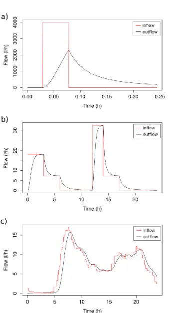
Figure 4 presents the results. A single event, like a bath emptying (case a), is considerably smoothed 125
by the septic tank. The outflow discharge reaches only 57% of the inflow rate at the end of loading. 126
Many treatment systems (e.g. sand filters) downstream of the septic tank have gravity-driven 127
distribution systems and therefore depend on inflow velocity to ensure an even distribution. If the 128
septic tank significantly smoothes its outflow discharge, this could affect the quality of hydraulic 129
distribution in the treatment system. When applied to more averaged hydrographs such as those 130
obtained synthetically based on daily hydraulic load and typical household water usage (AFNOR, 131
2013; case b) or those experimentally observed at sewer level (Butler & Gatt, 1996; case c), the 132
smoothing effect tends to be less significant: mean outflow discharges are only 0.6% and 3.75% lower 133
than mean inflow rates for the second and third test cases, respectively. In these cases, the septic tank 134
only induces a lag in the propagation of the hydrograph. In addition, case b shows that the septic tank 135
may help ensure a better spreading of hydraulic load over the day. 136
Evaluation of septic tank buffering on effluent distribution over the secondary treatment unit would 137
requires better measurements of the inlet hydrograph with a small time resolution. The hydrograph 138
suggested by (AFNOR, 2013) is too averaged and actually presents a shape close to the observed in 139
sewers. Patel et al. (2008) measured outflow at the inlet of gravity distribution devices (after the septic
140
tank) and concluded that the most common flow rates were between 0.0016-2.0.03 l h-1 with peak
141
values up to 0.2 l h-1. For secondary treatments that are not fed by gravity, the septic tank buffer effect 142
may help to ensure a better spreading of the influent over time. Furthermore, the current model could 143
be easily applied to septic tank alternative designs such as tank in series and tank in parallels as they 144
are already widespread in USA and tend to develop in Europe. A sensitivity analysis on parameters S
145
and D could also indicate which one influence the most buffer effect and lag time.
146
Finally, we would like to stress that not only septic tank induces a buffer effect. Pipes, conducting
147
flow to and out of the septic tank, may also be of importance regarding their diameter (typically 100
148
mm).
150
Figure 4. Inflow and outflow hydrographs for three test cases: a) bath emptying, b) synthetic daily dataset, c) dry
151
weather sewage flow (Butler & Gatt, 1996)
152
Conclusions
153
We built a simple mechanistic model suitable for modeling the hydraulic buffering induced by a septic 154
tank. The only constant in the model, i.e. the loss coefficient, was calibrated using deterministic CFD 155
modeling. Results highlight significant modulation of flow in single relatively large events such as a 156
bath emptying. However, on smoother hydrographs, such as those currently available for 157
characterizing a household effluent, the flow modulation only adds a lag time into the influent 158
hydrograph. As we progressively gain more knowledge on the actual shape and amplitude of the 159
hydrograph at the inlet of a septic tank, this simple tool could prove be useful for modeling septic tank 160
outflow and its impact on the spread of wastewater over the treatment unit in configurations based on 161
gravity-driven distribution. 162
References
163
AFNOR (2007). XP DTU 64.1. Mise en œuvre des dispositifs d’assainissement non collectif (dit 164
autonome). [in French] 165
AFNOR (2013) NF EN 12566-3. Petites installations de traitement des eaux uses jusqu’à 50 PTE – 166
partie 3 : stations d’épuration des eaux usées domestique prêtes à l’emploi et/ou assemblées sur site. 167
[in French]. 168
Brent, R. (1973). Algorithms for Minimization without Derivatives. Englewood Cliffs N.J., Prentice-169
Hall. 170
Bridson-Pateman, E., Hayward, J., Jamieson, R., Boutillier, L., Lake, C. (2013). The effects of dosed 171
versus gravity-fed loading methods on the performance and reliability of contour trench disposal fields 172
used for on-site wastewater treatment. Journal of Environmental Quality 42(2): 553-561. 173
Butler, D., Graham, N. (1995). Modeling dry weather wastewater flow in sewer networks. Journal Of 174
Environmental Engineering 121(2): 161-173. 175
Butler, D., Gatt, K. (1996). Synthesising dry weather flow input hydrographs: A Maltese case study. 176
Water Sci. Technol. 34 (3-4): 55-62. 177
Cauchi, A., Vignolles, C. (2012). Characteristics of raw water from the individual house. L’eau, 178
l’industrie, les nuisances. 354: 91-95. [in French]. 179
Gill, L.W., O’Luanaigh, N., Johnston, P.M., Misstear, B.D.R., O’Suilleabhain, C. (2009). Nutrient 180
loading on subsoils from on-site wastewater effluent, comparing septic tank and secondary treatment 181
systems. Water Research 43: 2739-2749. 182
Hager W. H. (1999). Wastewater hydraulics. Springer. 183
OpenFOAM (2013). OpenFOAM – The open source CFD toolbox – User guide. OpenFOAM 184
Foundation. 185
Patel, T, O’Luanaigh, N., Gill, L.W. (2008). A comparison of gravity distribution devices used in
on-186
site domestic wastewater treatment systems. Journal of Water, Air & Soil Pollution 191: 55-69.
187
R Core Team (2013). R: A language environment for statistical computing. R Foundation for 188
Statistical Computing, Vienna, Austria, URL http://www.R-project.org/. 189
Roland, L. (2009). Comparative analyses of seepage: clogging tools for the diagnosis. Université 190
Montpellier II, Sciences et Techniques du Languedoc, PhD Thesis, 224 pp. [in French]. 191
Vazquez, J., Zug, M., Bellefleur, D., Grandjean, B., Scrivener, O. (1999). Use of neural network to 192
apply the Muskingum model to sewer networks. Journal of Water Science 12(3): 577-595. 193
Winstanley, H.F., Fowler, A.C. (2013). Biomat development in soil treatment units for on-site 194
wastewater treatment. Bulletin of Mathematical Biology 75: 1985-2001. 195