Conditional Lower Bounds for Graph Sensitivity
Problems
by
Bertie Ancona
B.S., Massachusetts Institute of Technology (2018)
Submitted to the Department of Electrical Engineering and Computer Science
in Partial Fulfillment of the Requirements for the Degree of
Master of Engineering in Electrical Engineering and Computer Science
at the
MASSACHUSETTS INSTITUTE OF TECHNOLOGY
June 2019
c
○ Massachusetts Institute of Technology 2019. All rights reserved.
Author . . . .
Department of Electrical Engineering and Computer Science
June 7, 2019
Certified by . . . .
Virginia Vassilevska Williams
Associate Professor
Thesis Supervisor
Accepted by . . . .
Katrina LaCurts
Chair, Master of Engineering Thesis Committee
Conditional Lower Bounds for Graph Sensitivity Problems
by
Bertie Ancona
Submitted to the Department of Electrical Engineering and Computer Science on June 7, 2019, in partial fulfillment of the
requirements for the Degree of
Master of Engineering in Electrical Engineering and Computer Science
Abstract
In this thesis, we show conditional lower bounds for graph distance problems in the sensitivity setting, a restriction on the dynamic setting. We consider graph diameter, radius, and eccentricities over a few distance metrics, and sensitivities both constant and logarithmic in the size of the graph. Despite these restrictions, we find that many lower bound results from the static and fully dynamic settings still hold under popular conjectures. We show many of these lower bounds for graphs with constant maximum degree as well.
Thesis Supervisor: Virginia Vassilevska Williams Title: Associate Professor
Acknowledgments
I would like to thank my advisor Virginia V. Williams for all of her guidance and teaching (and chocolates) over the past year. I would also like to thank Nicole Wein for helpful discussions and proof debugging. Thanks to Magdalen and Kyle for their support through the process of researching and writing the thesis.
Contents
1 Introduction 13
1.1 Results . . . 14
1.1.1 Approximation in Undirected Graphs . . . 14
1.1.2 Approximation in Directed Graphs . . . 16
1.1.3 Finite Approximation in Directed Graphs . . . 17
1.2 Related Work . . . 18
2 Preliminaries 21 2.1 Notation and Problems Considered . . . 21
2.2 Conjectures . . . 23
2.3 Proof Ideas and Base Graphs . . . 24
2.3.1 SETH and 3HSH Reduction Outline and Base Graph 𝐺𝛿 . . . 24
2.3.2 𝑘CC Reduction Outline and Base Graph 𝐺𝑘 . . . 26
3 Approximation in Undirected Graphs 29 3.1 (2 − 𝜖)-Approximation Requires Linear Time . . . 29
3.2 (3/2 − 𝜖)-Approximation Requires Quadratic Time . . . 31
4 Approximation in Directed Graphs 39 4.1 Directed Diameter . . . 39
5 Finite Approximation in Directed Graphs 51 5.1 𝑘-Cycle Constructions . . . 51 5.2 SETH Construction for Min Radius and Eccentricity . . . 56
List of Figures
2-1 Sketch of 𝐺𝛿 construction . . . 25
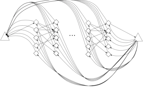
2-2 Sketch of 𝐺𝑘 construction . . . 27
3-1 Sketch of Theorem 3.2.1 construction . . . 32
3-2 Sketch of Theorem 3.2.2 construction . . . 34
4-1 Sketch of Theorem 4.1.2 construction . . . 41
4-2 Sketch of Theorem 4.2.1 construction . . . 44
List of Tables
1.1 Summary of Undirected Approximation Results . . . 16 1.2 Summary of Directed Approximation Results . . . 17 1.3 Summary of Finite Approximation Results . . . 18
Chapter 1
Introduction
Lower bounds on computational problems allow us to determine when an algorithm is optimal or close to it, but unconditional lower bounds can be difficult to determine for many problems. An alternative approach is to take a conjecture that some problem requires a particular running time, and to reduce this problem to others to show conditional lower bounds; that is, the lower bound of the problems are conditional on the assumption of the lower bound for the original problem. These conditional lower bounds can be much stronger than their unconditional counterparts, though they are weakened by the assumption made.
This thesis explores conditional lower bounds for graph eccentricities, diameter and radius in the sensitivity setting, a restriction on the dynamic setting. The eccentricity of a node is the largest shortest-path distance from that node to any other node. The diameter of a graph is simply the maximum of all eccentricities, and the radius is the minimum of all eccentricities. These distance problems are fundamental, and algorithms for them have been extensively studied in the static and dynamic settings. We consider a few notions of distance for these problems: one-way distance; maximum distance, where the distance between two nodes is the larger of the two one-way distances between those nodes; and minimum distance, where the distance is the smaller of the two one-way distances. These are all equivalent when the graph is undirected, but in a directed graph it is not clear that these are equivalently difficult to compute.
In the fully dynamic setting, an algorithm is allowed to preprocess its input for some polynomial amount of time, but then the input graph may be updated before queries to the algorithm. The updates considered in this thesis are graph edge additions and deletions, which may respectively decrease or increase distance between nodes in the graph.
The sensitivity setting is a type of dynamic setting in which algorithms can expect re-strictions on the updates received before a query. The updates come in small batches, and the size of the batch is termed the sensitivity of the problem. Updates are only performed on the original input; after a query, the algorithm rolls back to its original state after pre-processing. The updates are also only of one type: incremental, where only edge additions are allowed, or decremental, where only edge deletions are allowed.
One may expect that the restrictions of the sensitivity setting may make problems easier than the dynamic case. For example, determining the diameter of a graph after a constant number of edge additions seems like it could be easier than finding the diameter after edge additions in batches logarithmic in the size of the graph, or at least easier than after adding all edges of the graph. We further restrict the possible input graphs when possible to provide stronger lower bounds, by giving graph constructions that have constant maximum degree or are acyclic. Despite all of these restrictions, we show that in many cases, approximating the diameter, radius, or eccentricities in this setting is as hard as in the fully dynamic setting, or even as hard as recomputing the answer from scratch every update.
1.1
Results
1.1.1
Approximation in Undirected Graphs
Our main contribution is a construction showing the difficulty of approximating the above graph distance problems on undirected, unweighted graphs to any factor better than 2, assuming the Strong Exponential Time Hypothesis (SETH). (More information about con-jectures used in this thesis appears in section 2.2.) Under SETH, any algorithm guaranteeing a (2 − 𝜖)-approximation for any constant 𝜖 > 0 of diameter, radius, or single-vertex
eccentric-ity requires linear time per update or query on a sparse graph with 𝑛 nodes, even on graphs with constant maximum degree and restricting the sensitivity to 𝜔(log 𝑛). This improves on an earlier lower bound by Henzinger et al [9] for calculating diameter in 𝑛12−𝑜(1) time, which
applied only to weighted graphs in the fully dynamic setting.
An interesting feature of this construction is that it provides a lower bound for approxi-mating graph radius under SETH; we are unaware of a previous SETH reduction to radius. The difficulty of reducing from 𝑘-SAT to radius stems from the difference in quantifiers of the two problems: 𝑘-SAT (like diameter) has only existence quantifiers, because we wish to find the existence of a satisfying assignment, whereas radius has quantifiers ∃∀, because we wish to find the existence of a node which has a small distance to all other vertices.
We get around this difficulty by mirroring the constructed graph about a single, central node, which constrains all paths from one side of the graph to the other to pass through the central node. The central node thus has the minimum eccentricity of all nodes, and because the graph is mirrored and all paths must go through the central node, the diameter is simply twice the maximum distance from any node to the central node. In other words, the diameter is always exactly twice the radius of the graph. We use this graph mirroring technique for some of our finite approximation results as well.
A similar construction without constant-degree appeared [4], where it was shown that because the eccentricity of the central node is always the radius of the graph, the construction provides a way to show a lower bound for calculating the eccentricity of a single fixed vertex, instead of the eccentricities of all vertices in the graph as in some of our other constructions. We also extend previous results on the hardness of (3/2 − 𝜖)-approximate diameter and radius, and (5/3 − 𝜖)-approximate eccentricities. For diameter and eccentricities, we simply extend previous results [4] under SETH to graphs with constant maximum degree, and for radius, we extend static results [3], [8] to the sensitivity setting under a variant of the Hitting Set hypothesis. All of our constructions yield lower bounds of quadratic time per update or query with sensitivity 𝜔(log 𝑛) for sparse graphs with 𝑛 nodes.
Problem Approx. Sens. Lower Bounds Deg. Inc/Dec Conj. Ref. 𝑝(𝑛) 𝑢(𝑛), 𝑞(𝑛)
Diameter 3/2 − 𝜖 𝜔(log 𝑛) 𝑛𝑡 𝑛2−𝜖 𝑂(1) Inc/Dec SETH 3.2.1
2 − 𝜖 𝜔(log 𝑛) 𝑛𝑡 𝑛1−𝜖 𝑂(1) Inc/Dec SETH 3.1.1
Radius 3/2 − 𝜖 𝜔(log 𝑛) 𝑛𝑡 𝑛2−𝜖 𝑂(1) Inc/Dec 3HSH 3.2.2
2 − 𝜖 𝜔(log 𝑛) 𝑛𝑡 𝑛1−𝜖 𝑂(1) Inc/Dec SETH 3.1.1
Eccentricities 5/3 − 𝜖 𝜔(log 𝑛) 𝑛𝑡 𝑛2−𝜖 𝑂(1) Inc/Dec SETH 3.2.3
Fixed-Vertex
Eccentricity 2 − 𝜖 𝜔(log 𝑛) 𝑛
𝑡 𝑛1−𝜖 𝑂(1) Inc/Dec SETH 3.1.1
Table 1.1: A summary of our lower bound results for graph distance approximation prob-lems in undirected graphs.
1.1.2
Approximation in Directed Graphs
For directed graphs, we consider three different distance measures between nodes: one-way distance, min-distance, and max-distance. Distance in the real world is often asymmetric, so that the distance from location 𝑢 to 𝑣 is different from the distance from 𝑣 to 𝑢. Our results in this section are less complete, but begin to paint a picture of possible differences in complexity between the different variations of diameter and between diameter and radius. We note that the lower bound for undirected diameter applies also to one-way diameter (which is equivalent to max diameter) and min diameter, and we cannot hope to achieve a higher approximation ratio for one-way diameter with a quadratic time lower bound due to upper bounds for 3/2-approximation of ˜𝑂(𝑚3/2) by [7] and of ˜𝑂(𝑚𝑛1/2) by [13] (with
small additive error). However, we do extend a static result for min diameter by [3] to the sensitivity setting, showing that (2 − 𝜖)-approximation requires quadratic time per update or query with sensitivity 𝜔(log 𝑛) on weighted sparse graphs with 𝑛 nodes. Whether a similar lower bound exists for unweighted graphs remains unknown, though we suspect that it does. The variations of radius are more uniform in terms of run-time lower bounds. We extend from previous static results [3] to show that (2 − 𝜖)-approximation of any of the radius vari-ations requires quadratic time per update or query with sensitivity 𝜔(log 𝑛) on unweighted sparse graphs with 𝑛 nodes. These imply the same lower bounds for the various versions of eccentricities, because we may simply query all eccentricities and find the radius in linear
Problem Approx. Sens. Lower Bounds Deg. Inc/Dec Conj. Ref. 𝑝(𝑛) 𝑢(𝑛), 𝑞(𝑛) Diam and Min-Diam. 3/2 − 𝜖 𝜔(log 𝑛) 𝑛 𝑡 𝑛2−𝜖 𝑂(1) Inc/Dec SETH 4.1.1 Min-Diam. (Weighted) 2 − 𝜖 𝜔(log 𝑛) 𝑛 𝑡 𝑛2−𝜖 𝑂(1) Inc/Dec SETH 4.1.2 One-Way Rad.
and Eccs. 2 − 𝜖 𝜔(log 𝑛) 𝑛
𝑡 𝑛2−𝜖 𝑂(1) Inc/Dec 3HSH 4.2.1 Max-Rad. and Max-Eccs 2 − 𝜖 𝜔(log 𝑛) 𝑛 𝑡 𝑛2−𝜖 𝑂(1) Inc/Dec 3HSH 4.2.2 Min-Rad., Fixed-Vertex Min-Ecc. 2 − 𝜖 𝜔(log 𝑛) 𝑛𝑡 𝑛2−𝜖 𝑂(𝑛) Inc/Dec 3HSH 4.2.3
Table 1.2: A summary of our lower bound results for graph distance approximation prob-lems in directed graphs.
time afterward.
1.1.3
Finite Approximation in Directed Graphs
The previous two sections describe results suggesting that approximating diameter, radius, and eccentricities to within constant factors in the sensitivity setting requires linear or quadratic time. However, one could consider a more basic question: is the diameter or radius of a graph finite, or infinite? Depending on the distance metric we are using, infinite distance could mean that two vertices are not reachable from each other, or that one or both cannot reach the other. It seems feasible that such queries may be computed quite easily.
However, we show that for all of these distance variations, diameter, radius, and eccen-tricity of a fixed vertex require linear time per update or query, or quadratic preprocessing time, under the 𝑘-Cycle Conjecture (𝑘CC). These bounds hold for constant sensitivity and constant maximum degree, though they only hold in the incremental case. The construc-tions are based heavily on one appearing in [4] for fully dynamic finite approximation of diameter. We further show that even allowing arbitrary polynomial processing time, SETH implies that min-radius and min-eccentricity of a fixed vertex also requires linear update or query time, even with constant sensitivity and maximum degree. The constant sensitivity is
Problem Sens. Lower Bounds Deg. Inc/Dec Conj. Ref. 𝑝(𝑛) 𝑢(𝑛), 𝑞(𝑛)
Diam., Min-Diam., Fixed-Vertex Ecc. & Max-Ecc.
2 𝑛2−𝜖 𝑛1−𝜖 𝑂(1) Inc 𝑘CC 5.1.1 One-Way Rad. Max-Rad. 4 𝑛2−𝜖 𝑛1−𝜖 𝑂(1) Inc 𝑘CC 5.1.2.1 Min-Rad., Fixed-Vertex Min-Ecc. 5.1.2.2 Min-Rad., Fixed-Vertex Min-Ecc. 𝐾(𝜖, 𝑡) 𝑛𝑡 𝑛1−𝜖 𝑂(1) Inc/Dec SETH 5.2.1
Table 1.3: A summary of our lower bound results for graph distance finite-approximation problems in directed graphs.
a function of the 𝜖 and the preprocessing time of the algorithm, and uses a technique from [2] and [10] to reduce the sensitivity to a constant. We do not use this technique for our other constructions because it weakens the approximation guarantees, but in this case the approximation is finite either way.
Most of these constructions make use of the trick of mirroring the graph about one vertex in order to force all paths from one side of a symmetric graph to the other through the central vertex, guaranteeing that the central vertex is the center of the graph.
1.2
Related Work
In [10] many sensitivity results were shown, including that (4/3 − 𝜀)-approximation of the diameter or all ecentricities in sparse graphs requires 𝑛2−𝑜(1) time per update or per query
under the Boolean Matrix Multiplication conjecture and SETH, respectively. They also showed that (4/3 − 𝜖)-approximation of diameter with constant sensitivity requires linear team per update or query. [2] also showed a host of dynamic sensitivity lower bounds, including that (4/3 − 𝜀)-approximation of the diameter requires quadratic time per update or query under SETH, and provided the basis for a sensitivity reduction technique used in
[10].
In [4], the approximation ratios of lower bounds for diameter and eccentricities in the sensitivity setting were improved to 5/3 − 𝜖 and 3/2 − 𝜖 respectively. Sensitivity bounds were also shown for (2 − 𝜖)-approximate one-way radius, finite-approximate diameter, radius, and fixed-vertex eccentricities. Previous versions of constructions in this thesis also appeared, but the graphs did not have bounded degree.
In [9] many lower bounds in the fully dynamic setting based on the Online Matrix Vector (OMv) conjecture appeared. Particularly, they determined that the OMv conjecture implied a fully dynamic lower bound of 𝑛1/2−𝑜(1) per update or query for a (2 − 𝜀)-approximation of weighted diameter, but no previous sensitivity lower bound exists for this approximation ratio.
Our SETH constructions, both in the undirected and directed cases, extend or are inspired by the constructions from the above sources, and similar constructions appear in [1] and [6]. Under SETH, [13] showed that in the static case, (3/2−𝜖)-approximate diameter requires quadratic time, and [5] showed that (5/3 − 𝜖)-approximate diameter requires 𝑛1.5−𝑜(1) time. [7] showed that under SETH, (5/3 − 𝜖)-approximate eccentricities requires quadratic time. Under the balanced Hitting Set conjecture, [3] showed that static (3/2 − 𝜖)-approximation of radius requires 𝑛2−𝑜(1) time in unweighted, undirected graphs, and (2 − 𝜖)-approximation
of one-way, max-, and min-radius require 𝑛2−𝑜(1)time in unweighted, directed graphs. In [4], it was shown that (2 − 𝜖)-approximate one-way radius (termed source radius in the paper) requires quadratic time per update or query. Our constructions for these variants of radius build from and strengthen theirs to the sensitivity setting, with constant maximum degree. [8] showed quadratic lower bounds under SETH for (3/2 − 𝜖)-approximate diameter and radius and (5/3 − 𝜖)-approximate eccentricities in the static setting on unweighted, undi-rected sparse graphs where the maximum degree is bounded by a constant. [1] used similar degree reduction techniques, and [2] also used full binary trees in their dynamic lower bound constructions. We use similar techniques to reduce the maximum degree in many of our constructions.
Chapter 2
Preliminaries
2.1
Notation and Problems Considered
This section provides more formal definitions of the problems considered in this thesis, as well as notation used for clarity and brevity.
Graphs A graph 𝐺 consists of nodes 𝑉 and edges 𝐸 which are (possibly directed) pairs of nodes. We will sometimes refer to nodes as vertices. Unless otherwise defined, 𝑛 = |𝑉 | and 𝑚 = |𝐸|.
Sensitivity A dynamic graph algorithm is allowed some preprocessing time on the original graph, and then undergoes a series of updates to graph and queries to some property of the current graph. The algorithm is incremental if only edge insertions are allowed as updates, decremental if only edge deletions are allowed, and fully dynamic if the updates may be either edge insertions or deletions. An algorithm with sensitivity 𝜎 is either incremental or decremental, and after preprocessing undergoes only 𝜎 updates in a batch before a query. After a query, the algorithm rolls back to its state just after preprocessing.
Distance Let d(𝑢, 𝑣) denote the shortest one-way distance from 𝑢 to 𝑣, and let d𝑚𝑖𝑛(𝑢, 𝑣) =
𝑣, then d(𝑢, 𝑣) = ∞.
Approximation An algorithm for property 𝑃 is 𝛼-approximate if the value ˆ𝑃 it produces satisfies either 𝑃 ≤ ˆ𝑃 ≤ 𝛼𝑃 , or 𝛼𝑃 ≤ ˆ𝑃 ≤ 𝑃 . An algorithm produces a finite approximation if it distinguishes between finite and infinite values of 𝑃 .
Eccentricities Define the eccentricity of a node 𝑢 to be 𝑒𝑐𝑐(𝑢) = max𝑣∈𝑉 {d(𝑢, 𝑣)}, and let
min- and max-eccentricity be defined as 𝑒𝑐𝑐𝑚𝑖𝑛(𝑢) = max𝑣∈𝑉 {d𝑚𝑖𝑛(𝑢, 𝑣)} and 𝑒𝑐𝑐𝑚𝑎𝑥(𝑢) =
max𝑣∈𝑉 {d𝑚𝑎𝑥(𝑢, 𝑣)} respectively. We consider two eccentricity problems: calculating all
eccentricities of a graph, and calculating the eccentricity of a fixed node of a graph.
Diameter and Radius Let the diameter of a graph 𝐺 = (𝑉, 𝐸) be 𝐷 = max𝑢∈𝑉 {𝑒𝑐𝑐(𝑢)},
and let the min-diameter be 𝐷𝑚𝑖𝑛 = max𝑢∈𝑉 {𝑒𝑐𝑐𝑚𝑖𝑛(𝑢)}. Note that an analogous
max-diameter is equivalent to the max-diameter. Let the radius of a graph 𝐺 = (𝑉, 𝐸) be 𝑅 = min𝑢∈𝑉 {𝑒𝑐𝑐(𝑢)}, and let the min- and max-radius be 𝑅𝑚𝑖𝑛 = min𝑢∈𝑉 {𝑒𝑐𝑐𝑚𝑖𝑛(𝑢)} and
𝑅𝑚𝑎𝑥 = min𝑢∈𝑉 {𝑒𝑐𝑐𝑚𝑎𝑥(𝑢)} respectively.
Trees Let 𝑇𝑘, −𝑇→𝑘, 𝑇←−𝑘, and←𝑇→𝑘 be full binary trees with 2⌈log 𝑘⌉< 2𝑘 leaves, where:
∙ 𝑇𝑘 has undirected edges,
∙ −𝑇→𝑘 has directed edges going away from the root,
∙ ←𝑇−𝑘 has directed edges going toward the root, and
∙ ←𝑇→𝑘 has directed edges in both directions.
Denote a node in a tree 𝑇 as available if it is not connected to any node outside of 𝑇 . Let 𝑟(𝑇 ) be the root of tree 𝑇 , and let 𝐿(𝑇 ) be the set of leaves of tree 𝑇 . Note that the height of a tree 𝑇𝑘 is 𝑂(log 𝑘).
2.2
Conjectures
This section lays out the conjectures upon which the lower bounds of this thesis rely. 𝑘-SAT is a well-known, NP-complete problem that poses whether, given a Boolean for-mula 𝐹 in conjunctive normal form with 𝑘 literals per clause on 𝑛 variables, there is an assignment to the variables that satisfies 𝐹 . No algorithm has done significantly better than the trivial algorithm of trying every possible assignment in 𝑂(2𝑛poly(𝑛)) time, which led to the following conjecture:
Conjecture 2.2.1 ([11]). Strong Exponential Time Hypothesis (SETH): For each 𝜖 > 0, there exists a 𝑘 ∈ N such that no algorithm exists that solves 𝑘-SAT in time 𝑂(2(1−𝜖)𝑛poly(𝑛)).
It is equivalent to restrict the CNF formulas to 𝑂(𝑛) clauses, due to the sparsification lemma of [12]. We will sometimes find it simpler to use the 𝑘-Orthogonal Vectors problem (𝑘-OV) instead of 𝑘-SAT. The 𝑘-OV problem is as follows: given 𝑘 sets {𝑈𝑖}𝑖∈[𝑘] of Boolean
vectors of size 𝑑 = 𝜔(log 𝑛), does there exist a 𝑢𝑖 from each 𝑈𝑖 such that for all vector
coordinates 𝑐, ∏︀
𝑖∈[𝑘]𝑢𝑖[𝑐] = 0? [14] showed that, if SETH holds, then for all 𝜖 > 0, no
algorithm for 𝑘-OV exists on vector sets {𝑈𝑖}𝑖∈[𝑘] running in time (︀ ∏︀𝑖∈[𝑘]|𝑈𝑖|
)︀1−𝜖 .
Certain problems, notably graph radius, do not lend themselves well to using SETH, due to the quantifiers describing the 𝑘-SAT problem. For these problems, we will use a problem related to 3-OV, introduced in [4]: unbalanced 3-HS. The unbalanced 3-HS problem is as follows: given 𝑈, 𝑉, 𝑊 ⊂ {0, 1}𝑑 with |𝑈 | = 𝑛, |𝑉 | = 𝑛𝑎, |𝑊 | = 𝑛𝑏 for constants 𝑎, 𝑏 > 0, are there 𝑢 ∈ 𝑈 and 𝑤 ∈ 𝑊 such that for all 𝑣 ∈ 𝑉 , 𝑢 · 𝑣 · 𝑤 ̸= 0? This is similar to 3-OV except that the quantifier for the last set is changed to ∀. This leads to the following conjecture, which is also implied by the balanced QBF conjecture from [15]:
Conjecture 2.2.2 ([4]). Unbalanced 3-HS Hypothesis (3HSH): For each 𝜖 > 0, no algorithm exists that solves unbalanced 3-HS on sets 𝑈, 𝑉, 𝑊 ⊂ {0, 1}𝑑 in time 𝑂((|𝑈 | · |𝑉 | · |𝑊 |)1−𝜖).
For one version of radius, we show a lower bound for finite approximation under SETH; however, SETH is unwieldy for most of the versions of diameter, radius, and eccentricities for showing such lower bounds. We turn to another problem called 𝑘-cycle: given a directed
graph, is there a cycle in the graph of length 𝑘? The 𝑘-Cycle Conjecture, used previously in the lower bounds of [4] and , states the following:
Conjecture 2.2.3 ([4]). 𝑘-Cycle Conjecture (𝑘CC): for all 𝜖 > 0, there exists a 𝑘 such that no algorithm exists that solves 𝑘-cycle in a graph of 𝑛 vertices and 𝑚 edges in time 𝑂(𝑚2−𝜖).
2.3
Proof Ideas and Base Graphs
We will generally assume for the sake of contradiction that a dynamic (𝛼 − 𝜖)-approximation algorithm exists (for the appropriate value of 𝛼) for diameter, radius, or eccentricities with preprocessing time 𝑛𝑡, amortized update time 𝑛2−𝜖′ and query time 𝑛2−𝜖′, for positive numbers
𝜖, 𝜖′, and 𝑡. We define 𝛿 = 1−𝜖𝑡 ′.
Our constructions sometimes include a parameter 𝑎 such that the supposed (𝛼 − 𝜖)-approximation algorithm may distinguish between the existence or non-existence of an or-thogonal triple or hitting set in each stage. We usually set 𝑎 = 𝜔(log 𝑛) so that any constant number of traversals from the root to a leaf (or vice versa) of a tree of depth 𝑂(log 𝑛) will be dwarfed in distance by a single traversal of a path of length 𝑎; this allows the use of binary trees to reduce the degree of nodes, as in [8].
After construction, there will be a series of stages in which the graph is updated, the sensitivity algorithm is queried, then the graph is rolled back to its original state. The updates described will be incremental, though most of our SETH reductions may be easily extended to decremental as well. We will then argue runtime and correctness.
2.3.1
SETH and 3HSH Reduction Outline and Base Graph 𝐺
𝛿We usually begin with an instance of 3-OV or 3-HS with vector sets 𝑈 , 𝑉 , and 𝑊 such that |𝑈 | = |𝑉 | = 𝑁𝛿 and |𝑊 | = 𝑁1−2𝛿. We first discard degenerate vectors and coordinates: any
coordinates that are 0 for every vector in 𝑈 , every vector in 𝑉 , or every vector in 𝑊 , and any vectors that are all zeroes. Note that removing degenerate coordinates does not change the correct output value. If there is a degenerate vector in a 3-OV instance or in 𝑈 or 𝑊
in a 3-HS instance, the correct output value is always “yes", while if there is a degenerate vector in 𝑉 in a 3-HS instance, removing it does not change the correct output value.
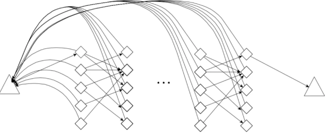
Construction of 𝐺𝛿 For each coordinate 𝑐, create two trees1 𝑇𝑁
𝛿
, and denote one by 𝑇𝑐𝑈
and the other by 𝑇𝑐𝑉. Next, create a path 𝜋(𝑢) of length 𝑎 for each vector 𝑢 ∈ 𝑈 ; denote
the 𝑖th node on the path by 𝜋(𝑢)𝑖, for 𝑖 in {0, . . . , 𝑎}. Add a tree 𝑇𝑢 = 𝑇𝑑 for each 𝑢, and
add an edge between 𝑟(𝑇𝑢) and 𝜋(𝑢)𝑎. We make a similar path 𝜋(𝑣) ending in a tree 𝑇𝑣 for
each 𝑣 ∈ 𝑉 . Encode each vector 𝑢 ∈ 𝑈 in the graph by adding a path of length 𝑎 between an available leaf of 𝑇𝑢 and an available leaf of 𝑇𝑐𝑈 iff 𝑢[𝑐] = 1. Encode each 𝑣 ∈ 𝑉 by adding
a path of length 𝑎 between an available leaf of 𝑇𝑣 and an available leaf of 𝑇𝑐𝑉 iff 𝑣[𝑐] = 1.
Figure 2-1: Sketch of 𝐺𝛿 construction. Bold edges represent paths, whose labels denote
their length. Triangles represent binary trees, and circles represent nodes.
Stages We proceed in 𝑁1−2𝛿 stages, one for each element 𝑤 ∈ 𝑊 . Generally, we will add
an edge to 𝐺𝛿 between 𝑟(𝑇𝑐𝑈) and 𝑟(𝑇𝑐𝑉) if 𝑤[𝑐] = 1, for all coordinates 𝑐. Then, we will
make a query to an algorithm we assume exists for the sake of contradiction. Depending on the result of the query, we will either detect an orthogonal vector triple or hitting set and halt, or we will undo our edge additions for this stage and continue to the next 𝑤.
Each stage may be modified to be decremental by initializing 𝐺𝛿 with edges between the
roots of each 𝑇𝑐𝑈, 𝑇𝑐𝑉 pair and removing the excess edges during each stage.
Analysis We prove correctness separately for each individual reduction. We note here that 𝐺𝛿 has constant maximum degree, as each binary tree has maximum degree 3 and all other
nodes are in paths, and all nodes have a constant number of additional edges.
The running time analysis is the same for all of the reductions from 3-OV and 3-HS. The preprocessing time of the algorithm for a graph of size ˜𝑂(𝑁𝛿) is ˜𝑂((𝑁𝛿)𝑡) = ˜𝑂(𝑁1−𝜖′). The
larger of the update or query time is 𝑂((𝑁𝛿)2−𝜖′), so after 𝑁1−2𝛿 stages wherein we make ˜
𝑂(1) updates and queries, the total time is ˜𝑂(𝑁1−𝛿𝜖′). This gives an algorithm for 3-OV or
3-HS in ˜𝑂(𝑁1−𝜖′ + 𝑁1−𝛿𝜖′) = 𝑂((|𝑈 ||𝑉 ||𝑊 |)1−𝜖′′) for a positive constant 𝜖′′, refuting SETH or 3HSH.
2.3.2
𝑘CC Reduction Outline and Base Graph 𝐺
𝑘We begin with an instance of 𝑘-cycle, with directed graph 𝐺 = (𝑉, 𝐸), where |𝑉 | = 𝑛 and |𝐸| = 𝑚 = ˜𝑂(𝑛). The lower bounds we prove with 𝑘-cycle are all for finite approximation algorithms, and unlike the SETH and 3HSH reductions, cannot easily be converted to decre-mental. The main idea is to create 𝑘 + 1 layers of 𝐺, so that there is a path from a node 𝑣 ∈ 𝑉 in the first layer to the copy of 𝑣 in the (𝑘 + 1)th layer iff 𝑣 participates in a 𝑘-cycle.
Construction We construct the base graph 𝐺𝑘 as follows, starting from an empty graph.
For each 𝑣 ∈ 𝑉 with in-degree 𝑑𝑒𝑔𝑖𝑛(𝑣) and out-degree 𝑑𝑒𝑔𝑜𝑢𝑡(𝑣), let
←− 𝑇𝑣 = ←−−−−−−−−−− 𝑇max {3,𝑑𝑒𝑔𝑖𝑛(𝑣)} and −→𝑇𝑣 = −−−−−−−−−−→
𝑇max {3,𝑑𝑒𝑔𝑜𝑢𝑡(𝑣)} (The tree must have at least 3 leaves to make later proofs easier).
Add 𝑘 + 1 copies each of ←𝑇−𝑣 and
− →
𝑇𝑣, denoted by
←−
𝑇𝑣𝑖 and −→𝑇𝑣𝑖 for 𝑖 ∈ [𝑘 + 1]. Also add trees 𝑇𝑠 =
←−−−−−
𝑇3(𝑘+1)𝑚 and 𝑇 𝑡 =
−−−−−→
𝑇3(𝑘+1)𝑚. For all 𝑖, add an edge from the root of ←𝑇−𝑖
𝑣 to the root of
− →
𝑇𝑣𝑖. For each edge 𝑢 → 𝑣 in 𝐸 and for all 𝑖, add an edge from an available leaf of −→𝑇𝑢𝑖 to an available leaf of ←−−𝑇𝑖+1
𝑣 , for all 𝑖. For each leaf ℓ of all
− → 𝑇𝑖
𝑣, add an edge from ℓ to an available
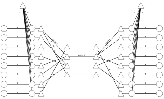
Figure 2-2: Sketch of 𝐺𝑘 construction. Diamond shapes represent two binary trees with
an edge between their roots.
Stages We proceed in 𝑛 stages, one for each element of 𝑉 . For the current 𝑣, we generally add to the graph an edge from 𝑟(𝑇𝑠) to any leaf of
←−
𝑇𝑣0 and an edge from any leaf of −𝑇→𝑘
𝑣 to 𝑟(𝑇𝑡) (if there are no such leaves, add the edges to or from the root of the trees),
then query the algorithm we assume exists for the sake of contradiction. If the queried value is infinite, we remove the edges we added in this stage and continue to the next 𝑣.
Analysis We prove correctness separately for each individual reduction, though we note that each node has degree at most three. All nodes are part of a tree ←𝑇 or− −→𝑇 and are either (1) roots of these trees, (2) leaves of these trees, or (3) neither. The construction of 𝐺𝑘 adds
at most a single edge to any root (1), at most two edges to any leaf (2), and no edges to any other node in the graph. Since roots begin with degree 2, leaves with degree 1, and all others with degree 3, all nodes in 𝐺′ have at most degree 3.
The running time analysis is roughly the same for all of the reductions from 𝑘CC. The graph has 𝑂(𝑘𝑚) = ˜𝑂(𝑛) nodes and edges. We perform 𝑂(𝑛) edge updates and 𝑛 queries, so the total update and query time is ˜𝑂(𝑛2−𝜖′). The preprocessing time is ˜𝑂(𝑛2−𝜖′) as well. For large 𝑘, this contradicts the 𝑘-cycle conjecture, which states that no algorithm exists for 𝑘-cycle in 𝑂(𝑛2−𝑓 (𝑘)−𝜖′′) time for any 𝜖′′ > 0 and any function 𝑓 that goes to 0 as 𝑘 goes to infinity.
Chapter 3
Approximation in Undirected Graphs
3.1
(2 − 𝜖)-Approximation Requires Linear Time
Theorem 3.1.1. Let 𝜖, 𝜖′, 𝑡 be positive constants. SETH implies that there exists no incre-mental or decreincre-mental dynamic algorithm for any of the following problems on undirected, unweighted graphs with 𝑛 vertices, ˜𝑂(𝑛) edges, and constant maximum degree which has sen-sitivity 𝜔(log 𝑛), preprocessing time 𝑝(𝑛) = 𝑛𝑡, and update time 𝑢(𝑛) and query time 𝑞(𝑛)
such that max {𝑢(𝑛), 𝑞(𝑛)} = 𝑛1−𝜖′:
∙ (2 − 𝜖)-approximate diameter, ∙ (2 − 𝜖)-approximate radius, and
∙ (2 − 𝜖)-approximate fixed-vertex eccentricity. Proof of Theorem 3.1.1.
Construction
Initialization Let 𝑎 = 𝜔(log 𝑁 ) and 𝛿 = 1−𝜖𝑡 . We begin with an instance of 2-OV with vector sets 𝑈 and 𝑉 of vectors of dimension 𝑑, with |𝑈 | = 𝑁𝛿 and |𝑉 | = 𝑁1−𝛿. We create
except instead of encoding elements of both 𝑈 and 𝑉 , we encode elements of 𝑈 twice to create a mirrored graph; denote one side by “left” and the other by “right”, instead of with “𝑈 ” and “𝑉 ” subscripts. Add also two trees 𝑇𝑠,𝑙𝑒𝑓 𝑡 = 𝑇𝑑 and 𝑇𝑠,𝑟𝑖𝑔ℎ𝑡 = 𝑇𝑑, and a node 𝑠 with
edges (𝑠, 𝑟(𝑇𝑠,𝑟𝑖𝑔ℎ𝑡) and (𝑠, 𝑟(𝑇𝑠,𝑟𝑖𝑔ℎ𝑡). We note that the graph has ˜𝑂(𝑁𝛿) nodes and edges.
Stages We proceed in 𝑁1−𝛿 stages, one for each element 𝑣 ∈ 𝑉 . For the current 𝑣, for
each coordinate 𝑐 where 𝑣[𝑐] = 1, we add an edge each from an available leaf of 𝑇𝑠,𝑙𝑒𝑓 𝑡 to
𝑟(𝑇𝑐𝑙𝑒𝑓 𝑡) and an available leaf of 𝑇𝑠,𝑟𝑖𝑔ℎ𝑡 to 𝑟(𝑇𝑐𝑟𝑖𝑔ℎ𝑡).
We then query the diameter or the radius of 𝐺 or the eccentricity of 𝑠. We will show that the eccentricity of 𝑠 is always equal to the radius, and we will show that if the diameter is least (8 + 𝑜(1)) · 𝑎 or the radius is at least (4 + 𝑜(1)) · 𝑎, then there is an orthogonal pair 𝑢, 𝑣; otherwise, the diameter is at most (4 + 𝑜(1)) · 𝑎 or the radius is at most (2 + 𝑜(1)) · 𝑎. We have set 𝑎 such that a (2 − 𝜖)-approximation algorithm for diameter or radius of 𝐺 or eccentricity of 𝑠 distinguishes between these two cases and can thus detect an orthogonal pair 𝑢, 𝑣 if one exists. If the query does not detect such an orthogonal pair, we undo the edge additions for the stage and continue to the next 𝑣.
We can modify the stage to be decremental by beginning with a matching between 𝐿(𝑇𝑠,𝑙𝑒𝑓 𝑡) and the set of roots of 𝑇𝑐𝑙𝑒𝑓 𝑡 and a matching between and 𝐿(𝑇𝑠,𝑟𝑖𝑔ℎ𝑡) and the roots
of 𝑇𝑐𝑟𝑖𝑔ℎ𝑡, and removing the excess edges each stage.
Analysis
Correctness We first claim that 𝑠 is always the center of 𝐺, so the eccentricity of 𝑠 and the radius of 𝐺 are always equal. Let 𝑥𝑟𝑖𝑔ℎ𝑡 be the node farthest from 𝑠 on the right
side of 𝐺. Since the graph is exactly symmetrical, the counterpart 𝑥𝑙𝑒𝑓 𝑡 of 𝑥𝑟𝑖𝑔ℎ𝑡 is such that
d(𝑠, 𝑥𝑟𝑖𝑔ℎ𝑡) = d(𝑠, 𝑥𝑙𝑒𝑓 𝑡). Any node 𝑦 to the left of 𝑠 must pass through 𝑠 to reach 𝑥𝑟𝑖𝑔ℎ𝑡, so
𝑦 must have a higher eccentricity than 𝑠 because it is farther from the node farthest from 𝑠. Symmetrically, any node 𝑦 to the right of 𝑠 must pass through 𝑠 to reach 𝑥𝑙𝑒𝑓 𝑡, so 𝑦 must
If for the current stage, for all 𝑢, 𝑢 · 𝑣 ̸= 0, then for each 𝑢 there must be some coordinate 𝑐 such that 𝑢[𝑐] = 𝑣[𝑐] = 1. Then there is a path of length 𝑂(log 𝑁 ) = 𝑜(𝑎) from 𝑠 to 𝑟(𝑇𝑐𝑙𝑒𝑓 𝑡), and a path of length 𝑂(log 𝑁 ) + 𝑎 + 𝑂(log 𝑑) = (1 + 𝑜(1)) · 𝑎 from 𝑟(𝑇𝑐𝑙𝑒𝑓 𝑡) to
𝜋(𝑢𝑙𝑒𝑓 𝑡)𝑎, for all 𝑢. The same is true on the right side. Then since all nodes are of distance
at most (1 + 𝑜(1)) · 𝑎 from some node 𝜋(𝑢𝑙𝑒𝑓 𝑡)𝑎 or 𝜋(𝑢𝑟𝑖𝑔ℎ𝑡)𝑎, all nodes are accessible in at
most (2 + 𝑜(1)) · 𝑎 steps from 𝑠. This means that the radius of 𝐺 and eccentricity of 𝑠 is (2 + 𝑜(1)) · 𝑎, and the diameter is at most (4 + 𝑜(1)) · 𝑎.
If for the current stage there is some 𝑢 such that 𝑢 · 𝑣 = 0, then there is no direct path from 𝑠 to 𝜋(𝑢)0 on either side via a tree 𝑇𝑐 and 𝜋(𝑢)𝑎. A path via a different 𝜋(𝑢′)𝑎 would
be of length at least (4 + 𝑜(1)) · 𝑎, because returning to a 𝑇𝑐′ where 𝑢[𝑐′] = 1 across two
length-𝑎 paths would cost at least an additional 2𝑎 from the direct path. Thus d(𝑠, 𝜋(𝑢)0)
would be at least (4 + 𝑜(1)) · 𝑎. The radius of 𝐺 and eccentricity of 𝑠 must then be at least (4 + 𝑜(1)) · 𝑎 and diameter must be at least (8 + 𝑜(1)) · 𝑎.
We note that the degree of all nodes is constant, because we only add binary trees to 𝐺𝛿
and add a constant number of edges for any node after that.
Running time We assume for the sake of contradiction that the algorithm of Theorem 3.1.1 exists. Let 𝑛 = ˜𝑂(𝑁𝛿) be the size of 𝐺. We have that max {𝑢(𝑛), 𝑞(𝑛)} = ˜𝑂((𝑁𝛿)1−𝜖′).
After initialization and |𝑉 | = 𝑁1−𝛿 stages, the total update and query time is then at most ˜
𝑂(𝑁1−𝛿𝜖′). The preprocessing time 𝑝(𝑛) for the algorithm on 𝐺 is ˜𝑂((𝑁𝛿)𝑡) = ˜𝑂(𝑁1−𝜖′).
Thus the total time of the algorithm is ˜𝑂(𝑁1−𝜖′ + 𝑁1−𝛿𝜖′). This contradicts SETH, because SETH implies that no algorithm exists for 2-OV in 𝑂((|𝑈 | · |𝑉 |)1−𝜖′′) = 𝑂(𝑁1−𝜖′′) time for
any 𝜖′′ > 0.
3.2
(3/2 − 𝜖)-Approximation Requires Quadratic Time
Theorem 3.2.1. Let 𝜖, 𝜖′, 𝑡 be positive constants. SETH implies that there exists no incre-mental or decreincre-mental dynamic algorithm for (3/2 − 𝜖)-approximate diameter on undirected,
unweighted graphs with 𝑛 vertices, ˜𝑂(𝑛) edges, and constant maximum degree which has sen-sitivity 𝜔(log 𝑛), preprocessing time 𝑝(𝑛) = 𝑛𝑡, and update time 𝑢(𝑛) and query time 𝑞(𝑛)
such that max {𝑢(𝑛), 𝑞(𝑛)} = 𝑛2−𝜖′. Proof of Theorem 3.2.1.
Construction
Initialization Let 𝑎 = 𝜔(log 𝑁 ) and 𝛿 = 1−𝜖𝑡 . We begin with an instance of 3-OV and construct a graph 𝐺 by first creating 𝐺𝛿 from subsection 2.3.1. We add two trees 𝑇𝑥= 𝑇𝑁
𝛿
and 𝑇𝑦 = 𝑇𝑁
𝛿
. For each node 𝑢 ∈ 𝑈 , add a path of length 𝑎 between 𝜋(𝑢)𝑎 and an available
leaf of 𝑇𝑥. Do the same between nodes 𝜋(𝑣)𝑎 and available leaves of 𝑇𝑦.
Figure 3-1: Sketch of Theorem 3.2.1 construction. Bold edges represent paths, whose labels denote their length.
Stages We proceed in 𝑁2−𝛿 stages, one for each element 𝑤 ∈ 𝑊 . For the current 𝑤,
for each coordinate 𝑐 where 𝑤[𝑐] = 1, we add an edge between 𝑟(𝑇𝑐𝑈) and 𝑟(𝑇𝑐𝑉). We then
query the diameter of 𝐺. We will show that if there is an orthogonal triple that includes 𝑤, then the diameter is least (6 + 𝑜(1)) · 𝑎, and otherwise, the diameter is at most (4 + 𝑜(1)) · 𝑎.
A (3/2 − 𝜖)-approximation algorithm for diameter distinguishes between these two cases and can thus detect an orthogonal triple that includes 𝑤 if one exists. If such an orthogonal triple is not detected, we undo the edge additions for the stage and continue to the next 𝑤. We can modify the stage to be decremental by beginning with a matching between {𝑟(𝑇𝑐𝑈) | 𝑐 ∈ [𝑑]} and {𝑟(𝑇𝑐𝑉) | 𝑐 ∈ [𝑑]}, and removing the excess edges each stage.
Analysis
Correctness If for the current stage, for all 𝑢 ∈ 𝑈 , 𝑣 ∈ 𝑉 , 𝑢 · 𝑣 · 𝑤 ̸= 0, then for each 𝑢, 𝑣 there exists a coordinate 𝑐 such that 𝑢[𝑐] = 𝑣[𝑐] = 𝑤[𝑐] = 1. Thus, for all 𝑢 and 𝑣, d(𝜋(𝑢)𝑎, 𝜋(𝑣)𝑎) = (2+𝑜(1))·𝑎 via 𝑇𝑢, the path between 𝑇𝑢and 𝑇𝑐𝑈, the edge between 𝑇𝑐𝑈 and
𝑇𝑐𝑉, and the path between 𝑇𝑐𝑉 and 𝑇𝑣. Also, for all 𝑢, 𝑢
′ ∈ 𝑈 , d(𝜋(𝑢)
𝑎, 𝜋(𝑢′)𝑎) ≤ (2 + 𝑜(1)) · 𝑎
via 𝑇𝑥, and for all 𝑣, 𝑣′ ∈ 𝑉 , d(𝜋(𝑢)𝑎, 𝜋(𝑢′)𝑎) ≤ (2 + 𝑜(1)) · 𝑎 via 𝑇𝑦. We note that every
vertex in the graph is of distance at most (1 + 𝑜(1)) · 𝑎 from some vertex 𝜋(𝑢)𝑎 or 𝜋(𝑣)𝑎.
Thus, the diameter is at most (4 + 𝑜(1)) · 𝑎.
Suppose for the current stage there exist 𝑢 ∈ 𝑈 , 𝑣 ∈ 𝑉 such that 𝑢 · 𝑣 · 𝑤 = 0. Fix 𝑢 and 𝑣. We claim that d(𝜋(𝑢)0, 𝜋(𝑣)0) ≥ (6 + 𝑜(1)) · 𝑎. The only paths between 𝜋(𝑢)0 and 𝜋(𝑣)0 go
through 𝜋(𝑢)𝑎and 𝜋(𝑣)𝑎. There does not exist a coordinate such that 𝑢[𝑐] = 𝑣[𝑐] = 𝑤[𝑐] = 1,
so every path between 𝜋(𝑢)𝑎 and 𝜋(𝑣)𝑎 must visit a vertex 𝜋(𝑢′ ̸= 𝑢)𝑎 or 𝜋(𝑣′ ̸= 𝑣)𝑎 which
are of distance (2 + 𝑜(1)) · 𝑎 from 𝜋(𝑢)𝑎 and 𝜋(𝑣)𝑎, respectively. The (2 + 𝑜(1)) · 𝑎 distance
from any 𝜋(𝑢′)𝑎 to any 𝜋(𝑣′)𝑎 must also be crossed. Thus, d(𝜋(𝑢)𝑎, 𝜋(𝑣)𝑎) ≥ (4 + 𝑜(1)) · 𝑎 so
d(𝜋(𝑢)0, 𝜋(𝑣)0) ≥ (6 + 𝑜(1)) · 𝑎.
The maximum degree is still constant in this construction, as only binary trees and paths are added to 𝐺𝛿 and constant additional edges are added to any particular node.
Running time 𝐺 is of size ˜𝑂(𝑁𝛿) with ˜𝑂(𝑁𝛿) edges, and we perform ˜𝑂(1) updates
Theorem 3.2.2. Let 𝜖, 𝜖′, 𝑡 be positive constants. 3HSH implies that there exists no incre-mental or decreincre-mental dynamic algorithm for (3/2 − 𝜖)-approximate radius on undirected, unweighted graphs with 𝑛 vertices, ˜𝑂(𝑛) edges, and constant maximum degree which has sen-sitivity 𝜔(log 𝑛), preprocessing time 𝑝(𝑛) = 𝑛𝑡, and update time 𝑢(𝑛) and query time 𝑞(𝑛)
such that max {𝑢(𝑛), 𝑞(𝑛)} = 𝑛2−𝜖′. Proof of Theorem 3.2.2.
Construction
Initialization Let 𝑎 = 𝜔(log 𝑁 ) and 𝛿 = 1−𝜖𝑡 . We begin with an instance of 3-HS and construct a graph 𝐺 by first creating two copies of the graph from Theorem 3.2.1; call these copies 𝐺𝑙𝑒𝑓 𝑡 and 𝐺𝑟𝑖𝑔ℎ𝑡. 𝐺 will be the graph composed of 𝐺𝑙𝑒𝑓 𝑡 and 𝐺𝑟𝑖𝑔ℎ𝑡, where for each
𝑢 ∈ 𝑈 , we merge the vertex 𝜋(𝑢𝑙𝑒𝑓 𝑡)0 in 𝐺𝑙𝑒𝑓 𝑡 with the vertex 𝜋(𝑢𝑟𝑖𝑔ℎ𝑡)0 in 𝐺𝑟𝑖𝑔ℎ𝑡; denote this
node by 𝜋(𝑢)0.
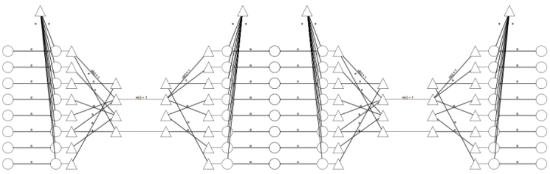
Figure 3-2: Sketch of Theorem 3.2.2 construction. Bold edges represent paths, whose labels denote their length.
Stages We proceed in 𝑁2−𝛿 stages, one for each element 𝑤 ∈ 𝑊 . For the current 𝑤,
for each coordinate 𝑐 where 𝑤[𝑐] = 1, we add an edge between 𝑟(𝑇𝑐𝑈,𝑙𝑒𝑓 𝑡) and 𝑟(𝑇𝑐𝑉,𝑙𝑒𝑓 𝑡), and
do the same on the right side. We then query the radius of 𝐺. We will show that if there is a hitting set that includes 𝑤, then the radius is at most (4 + 𝑜(1)) · 𝑎, and otherwise, the radius is at least (6 + 𝑜(1)) · 𝑎. A (3/2 − 𝜖)-approximation algorithm for radius distinguishes between these two cases and can thus detect a hitting set that includes 𝑤 if one exists. If
such a hitting set is not detected, we undo the edge additions for the stage and continue to the next 𝑤.
We can modify the stage to be decremental by beginning with a matching between {𝑟(𝑇𝑐𝑈,𝑙𝑒𝑓 𝑡) | 𝑐 ∈ [𝑑]} and {𝑟(𝑇𝑐𝑉,𝑙𝑒𝑓 𝑡) | 𝑐 ∈ [𝑑]} and a matching between {𝑟(𝑇𝑐𝑈,𝑟𝑖𝑔ℎ𝑡) | 𝑐 ∈ [𝑑]}
and {𝑟(𝑇𝑐𝑉,𝑟𝑖𝑔ℎ𝑡) | 𝑐 ∈ [𝑑]}, and removing the excess edges each stage.
Analysis
Correctness Suppose there is a hitting set {𝑢, 𝑤} for the current stage. We will show that the node 𝜋(𝑢)0 is of distance at most (4 + 𝑜(1)) · 𝑎 from every other node. The node
𝜋(𝑢)0 can reach 𝜋(𝑢)𝑎 on either side in 𝑎 steps, and for all other 𝑢′ ∈ 𝑈 , d(𝜋(𝑢)0, 𝜋(𝑢′)𝑎) ≤
(3 + 𝑜(1)) · 𝑎 for 𝜋(𝑢′)𝑎 on either side of the graph, via 𝑇𝑥,𝑙𝑒𝑓 𝑡or 𝑇𝑥,𝑟𝑖𝑔ℎ𝑡. Since 𝑢 and 𝑤 define
a hitting set, for all 𝑣 there is a coordinate 𝑐 such that 𝑢[𝑐] = 𝑣[𝑐] = 𝑤[𝑐] = 1. Thus by the same argument as Theorem 3.2.1, d(𝜋(𝑢)𝑎, 𝜋(𝑣𝑙𝑒𝑓 𝑡)𝑎) = (2 + 𝑜(1)) · 𝑎 for all 𝑣, and the
same for the right side. This implies that 𝜋(𝑢)0 has a path of length (3 + 𝑜(1)) · 𝑎 to all
𝜋(𝑣)𝑎 on both sides of the graph. We note that all nodes are at distance (1 + 𝑜(1)) · 𝑎 from
some node 𝜋(𝑢′)𝑎 or 𝜋(𝑣′)𝑎, either on the left or right side of the graph. Then the radius
𝑅 ≤ 𝑒𝑐𝑐(𝜋(𝑢)0) = (4 + 𝑜(1)) · 𝑎.
Suppose there is no hitting set involving the current 𝑤 and any 𝑢. Fix a side of the graph (we will omit subscripts left and right ). The only paths between any 𝜋(𝑢)0 and any 𝜋(𝑣)0
go through 𝜋(𝑢)𝑎 and 𝜋(𝑣)𝑎 (on the appropriate side of the graph). For all 𝑢, there exists a
𝑣 such that there does not exist a coordinate 𝑐 with 𝑢[𝑐] = 𝑣[𝑐] = 𝑤[𝑐] = 1; in other words, 𝑢, 𝑣, 𝑤 form an orthogonal triple. Then by a similar argument as Theorem 3.2.1, any 𝜋(𝑢)0
is at distance at least (6 + 𝑜(1)) · 𝑎 from 𝜋(𝑣)0. All other nodes have a higher eccentricity
than some 𝜋(𝑢)0, because they must travel via some 𝜋(𝑢)0 to the other side of the graph and
are thus farther from 𝜋(𝑢)0’s farthest node (of which it has at least one on either side of the
graph, by symmetry). Thus, the radius must be at least (6 + 𝑜(1)) · 𝑎.
The maximum degree of the construction is still constant, as we simply mirror the con-stant maximum degree graph in Theorem 3.2.1.
Running time 𝐺 is of size ˜𝑂(𝑁𝛿) with ˜𝑂(𝑁𝛿) edges, and we perform ˜𝑂(1) updates
and queries each stage, so the running time argument from subsection 2.3.1 holds.
Theorem 3.2.3. Let 𝜖, 𝜖′, 𝑡 be positive constants. SETH implies that there exists no in-cremental or dein-cremental dynamic algorithm for (5/3 − 𝜖)-approximate all eccentricities on undirected, unweighted with 𝑛 vertices, ˜𝑂(𝑛) edges, and constant maximum degree which has sensitivity 𝜔(log 𝑛), preprocessing time 𝑝(𝑛) = 𝑛𝑡, and update time 𝑢(𝑛) and query time 𝑞(𝑛) such that max {𝑢(𝑛), 𝑞(𝑛)} = 𝑛2−𝜖′.
Proof of Theorem 3.2.3.
Construction
Initialization Let 𝑎 = 𝜔(log 𝑁 ) and 𝛿 = 1−𝜖𝑡 . We begin with an instance of 3-OV and construct a graph 𝐺 by first creating 𝐺𝛿 from subsection 2.3.1. We add tree 𝑇𝑥 = 𝑇𝑁
𝛿
. For each 𝑢 ∈ 𝑈 , add an edge between 𝜋(𝑢)0 and an available leaf of 𝑇𝑥.
Stages We proceed in 𝑁2−𝛿 stages, one for each element 𝑤 ∈ 𝑊 . For the current 𝑤,
for each coordinate 𝑐 where 𝑤[𝑐] = 1, we add an edge between 𝑟(𝑇𝑐𝑈) and 𝑟(𝑇𝑐𝑉). We then
query all eccentricities of 𝐺. We will show that if there is an orthogonal triple 𝑢, 𝑣, 𝑤, then 𝑒𝑐𝑐(𝜋(𝑢)𝑎) = (5 + 𝑜(1)) · 𝑎, and otherwise, 𝑒𝑐𝑐(𝜋(𝑢)𝑎) = (3 + 𝑜(1)) · 𝑎 for all 𝑢. A (5/3 −
𝜖)-approximation algorithm for all eccentricities distinguishes between these two cases and can thus detect an orthogonal triple that includes 𝑤 if one exists. If such an orthogonal triple is not detected, we undo the edge additions for the stage and continue to the next 𝑤.
We can modify the stage to be decremental by beginning with a matching between {𝑟(𝑇𝑐𝑈) | 𝑐 ∈ [𝑑]} and {𝑟(𝑇𝑐𝑉) | 𝑐 ∈ [𝑑]}, and removing the excess edges each stage.
Correctness If for the current stage, for all 𝑢 ∈ 𝑈 , 𝑣 ∈ 𝑉 , 𝑢 · 𝑣 · 𝑤 ̸= 0, then for each 𝑢, 𝑣 there exists a coordinate 𝑐 such that 𝑢[𝑐] = 𝑣[𝑐] = 𝑤[𝑐] = 1. Thus, for all 𝑢 and 𝑣, d(𝜋(𝑢)𝑎, 𝜋(𝑣)𝑎) = (2 + 𝑜(1)) · 𝑎 via 𝑇𝑢, 𝑇𝑐𝑈, 𝑇𝑐𝑉, and 𝑇𝑣. This implies that the
distance from 𝜋(𝑢)𝑎 to 𝜋(𝑣)0 is at most (3 + 𝑜(1)) · 𝑎, for all 𝑢 and 𝑣. Also, for all 𝑢, 𝑢′ ∈ 𝑈 ,
d(𝜋(𝑢)𝑎, 𝜋(𝑢′)𝑎) = (2+𝑜(1))·𝑎 via 𝑇𝑥. Thus the eccentricities of 𝜋(𝑢)𝑎are at most (3+𝑜(1))·𝑎
for all 𝑢.
Suppose for the current stage there exist 𝑢 ∈ 𝑈 , 𝑣 ∈ 𝑉 such that 𝑢 · 𝑣 · 𝑤 = 0. Fix 𝑢 and 𝑣. We claim that d(𝜋(𝑢)𝑎, 𝜋(𝑣)0) ≥ (5 + 𝑜(1)) · 𝑎. The only paths between 𝜋(𝑢)𝑎 and 𝜋(𝑣)0
go through 𝜋(𝑣)𝑎. There does not exist a coordinate such that 𝑢[𝑐] = 𝑣[𝑐] = 𝑤[𝑐] = 1, so
every path between 𝜋(𝑢)𝑎 and 𝜋(𝑣)𝑎must visit a vertex 𝜋(𝑢′ ̸= 𝑢)𝑎or 𝜋(𝑣′ ̸= 𝑣)𝑎which are of
distance at least (2 + 𝑜(1)) · 𝑎 from 𝜋(𝑢)𝑎 and 𝜋(𝑣)𝑎, respectively. The (2 + 𝑜(1)) · 𝑎 distance
from any 𝜋(𝑢′)𝑎 to any 𝜋(𝑣′)𝑎 must also be crossed. Thus, d(𝜋(𝑢)𝑎, 𝜋(𝑣)𝑎) ≥ (4 + 𝑜(1)) · 𝑎 so
d(𝜋(𝑢)𝑎, 𝜋(𝑣)0) ≥ (5 + 𝑜(1)) · 𝑎.
The construction does not increase the degree of any node from 𝐺𝛿 by more than a
constant, and only adds a binary tree, so the graph has constant degree.
Running time 𝐺 is of size ˜𝑂(𝑁𝛿) with ˜𝑂(𝑁𝛿) edges, and we perform ˜𝑂(1) updates
Chapter 4
Approximation in Directed Graphs
4.1
Directed Diameter
Note that the three variants of distance are all equivalent in undirected graphs or graphs where 𝑢 → 𝑣 implies 𝑣 → 𝑢. Thus we may reduce undirected diameter to any of its directed variants by replacing each edge with two directed edges.
Corollary 4.1.1. SETH implies the same lower bound as in Theorem 3.2.1 for the following problems on directed, unweighted sparse graphs with constant maximum degree:
∙ (3/2 − 𝜖)-approximate one-way diameter, ∙ (3/2 − 𝜖)-approximate min-diameter, and ∙ (3/2 − 𝜖)-approximate max-diameter.
However, we prove a stronger result for weighted min-diameter, based on a construction of [3]:
Theorem 4.1.2. Let 𝜖, 𝜖′, 𝑡 be positive constants. SETH implies that there exists no incre-mental or decreincre-mental dynamic algorithm for (2 − 𝜖)-approximate min-diameter on directed, weighted graphs with 𝑛 vertices, ˜𝑂(𝑛) edges, and constant maximum degree which has sen-sitivity 𝜔(log 𝑛), preprocessing time 𝑝(𝑛) = 𝑛𝑡, and update time 𝑢(𝑛) and query time 𝑞(𝑛)
Proof of Theorem 4.1.2.
Construction
Initialization Let 𝑎 = 𝜔(log 𝑁 ) and 𝛿 = 1−𝜖𝑡 . We begin with an instance of 3-OV and construct a graph 𝐺 by first creating 𝐺𝛿 from subsection 2.3.1. First, replace all undirected
edges with directed edges in both directions of weight 1. Next, remove all nodes 𝜋(𝑢)𝑖 and
𝜋(𝑣)𝑖 for all 𝑖 ∈ [𝑑], 𝑢 ∈ 𝑈 , and 𝑣 ∈ 𝑉 . Replace the length-𝑎 paths encoding the vectors 𝑈
and 𝑉 in 𝐺𝛿 with single edges of weight 𝑎, directed from the leaves of 𝑇𝑢 to the leaves 𝑇𝑐𝑈
and from the leaves of 𝑇𝑐𝑉 to the leaves of 𝑇𝑣.
Add a tree 𝑇𝑧 =
←→
𝑇𝑑. For each 𝑐 ∈ [𝑑] add edges 𝑟(𝑇𝑐𝑈) ↔ 𝐿(𝑇𝑧)𝑐 (i.e. the 𝑐th leaf of 𝑇𝑧)
and edges 𝑟(𝑇𝑐𝑉) ↔ 𝐿(𝑇𝑧)𝑐 all of weight 𝑎.
Add a tree 𝑇𝑥 =
←−−→
𝑇𝑑+𝑁𝛿. For each 𝑐 ∈ [𝑑], add edge 𝑟(𝑇𝑐𝑈) → 𝐿(𝑇𝑥)𝑐 and edge 𝑟(𝑇𝑐𝑉) →
𝐿(𝑇𝑥)𝑐 all of weight 1. For each 𝑢 ∈ 𝑈 , let ℓ be an available leaf of 𝑇𝑥. Add edge 𝑟(𝑇𝑢) → ℓ
of weight 1 and edge ℓ → 𝑟(𝑇𝑢) of weight 2𝑎.
Add a tree 𝑇𝑦 =
←−−→ 𝑇𝑑+𝑁𝛿
. For each 𝑐 ∈ [𝑑], add edge 𝐿(𝑇𝑦)𝑐 → 𝑟(𝑇𝑐𝑈) and edge 𝐿(𝑇𝑦)𝑐→
𝑟(𝑇𝑐𝑉), all of weight 1. For each 𝑣 ∈ 𝑉 , let ℓ be an available leaf of 𝑇𝑦. Add edge ℓ → 𝑟(𝑇𝑣)
of weight 1 and edge 𝑟(𝑇𝑣) → ℓ of weight 2𝑎.
Finally, add edge 𝑟(𝑇𝑦) → 𝑟(𝑇𝑥) of weight 1.
Stages We proceed in 𝑁2−𝛿 stages, one for each element 𝑤 ∈ 𝑊 . For the current 𝑤, for each coordinate 𝑐 where 𝑤[𝑐] = 1, add edge 𝑟(𝑇𝑐𝑈) → 𝑟(𝑇𝑐𝑉) of weight 1. We then query
the min-diameter of 𝐺. We will show that if there is an orthogonal triple that includes 𝑤, then the min-diameter is least (4 + 𝑜(1)) · 𝑎, and otherwise, the min-diameter is at most (2 + 𝑜(1)) · 𝑎. A (2 − 𝜖)-approximation algorithm for min-diameter distinguishes between these two cases and can thus detect an orthogonal triple that includes 𝑤 if one exists. If such an orthogonal triple is not detected, we undo the edge additions for the stage and continue to the next 𝑤.
Figure 4-1: Sketch of Theorem 4.1.2 construction. Bold edges represent edges with weight greater than 1, and dotted lines represent edges in either direction where the weights are different in each direction. The labels of edges denote their weight.
{𝑟(𝑇𝑐𝑈) | 𝑐 ∈ [𝑑]} to {𝑟(𝑇𝑐𝑉) | 𝑐 ∈ [𝑑]} of weight-1 edges, and removing the excess edges each
stage.
Analysis
Correctness First we note that all trees in the construction are bidirected and have height 𝑜(𝑎), so reaching any node in a tree is roughly equivalent to reaching any node in the tree. We claim that the min-distance between all nodes in the graph and any node in 𝑇𝑥,𝑇𝑦,𝑇𝑧, all 𝑇𝑐𝑈, and all 𝑇𝑐𝑉 is at most (2 + 𝑜(1)) · 𝑎:
∙ 𝑇𝑥 is at min-distance 𝑜(𝑎) from all 𝑇𝑐𝑈, all 𝑇𝑐𝑉, and 𝑇𝑦 via edges between leaves of
these trees, and min-distance (1 + 𝑜(1)) · 𝑎 from 𝑇𝑧 via any 𝑇𝑐 tree. There are edges to
𝑇𝑥 directly from all 𝑇𝑢 of weight 1, and edges from all 𝑇𝑣 to 𝑇𝑦 of weight 2𝑎, which is
∙ 𝑇𝑦 has edges to all 𝑇𝑣 from its leaves of weight 1, edges of weight 1 from its leaves to
the 𝑇𝑐𝑈 and 𝑇𝑐𝑉, and from there edges of weight 𝑎 to 𝑇𝑧. 𝑇𝑦 can reach 𝑇𝑥 via the edge
between their roots, and from there reach all 𝑇𝑢 via the weight-2𝑎 edges from 𝑇𝑥 to
the 𝑇𝑢.
∙ 𝑇𝑧 has weight-𝑎 edges from its leaves to the roots of the 𝑇𝑐𝑈 and 𝑇𝑐𝑉, and from the 𝑇𝑐𝑉
may reach the 𝑇𝑣 in (1 + 𝑜(1)) · 𝑎 more distance. The 𝑇𝑢 may reach 𝑇𝑧 via the weight-𝑎
edges to the 𝑇𝑐𝑈 and from there the weight-𝑎 edges to 𝑇𝑧.
∙ All 𝑇𝑐𝑈 and 𝑇𝑐𝑉 are reachable by all 𝑇𝑣 in distance (2 + 𝑜(1)) · 𝑎 via 𝑇𝑦, and all 𝑇𝑐𝑈 and
𝑇𝑐𝑉 may reach all 𝑇𝑢 in distance (2 + 𝑜(1)) · 𝑎 via 𝑇𝑥.
If for the current stage, for all 𝑢 ∈ 𝑈 , 𝑣 ∈ 𝑉 , 𝑢 · 𝑣 · 𝑤 ̸= 0, we will show that the min-distance between any pair of nodes is at most (2 + 𝑜(1)) · 𝑎. We need only consider a node in some 𝑇𝑢 and one in some 𝑇𝑣, as all other nodes are close, as shown above. For each 𝑢, 𝑣 there
exists a coordinate 𝑐 such that 𝑢[𝑐] = 𝑣[𝑐] = 𝑤[𝑐] = 1. Thus there is a length-(2 + 𝑜(1)) · 𝑎 path from 𝑇𝑢 to 𝑇𝑣 via the weight-𝑎 edge from a leaf of 𝑇𝑢 to one of 𝑇𝑐𝑈, the edge from 𝑟(𝑇𝑐𝑈)
to 𝑟(𝑇𝑐𝑉), and the weight-𝑎 edge from a leaf of 𝑇𝑐𝑉 to one of 𝑇𝑣. Thus the min-diameter of
𝐺 is at most (2 + 𝑜(1)) · 𝑎.
Suppose for the current stage there exist 𝑢 ∈ 𝑈 , 𝑣 ∈ 𝑉 such that 𝑢 · 𝑣 · 𝑤 = 0. Fix 𝑢 and 𝑣. We claim that d𝑚𝑖𝑛(𝑟(𝑇𝑢), 𝑟(𝑇𝑣)) ≥ (4 + 𝑜(1)) · 𝑎. There does not exist a coordinate such
that 𝑢[𝑐] = 𝑣[𝑐] = 𝑤[𝑐] = 1, so every path from 𝑟(𝑇𝑢) to 𝑟(𝑇𝑣) must visit a vertex 𝑟(𝑇𝑢′̸=𝑢)
via 𝑇𝑥 or 𝑟(𝑇𝑣′̸=𝑣) via 𝑇𝑦, both of which incur (2 + 𝑜(1)) · 𝑎 distance leaving or entering 𝑇𝑥 and
𝑇𝑦 respectively; or the path must go through some 𝑇𝑐′̸=𝑐 via 𝑇𝑧, which incurs (2 + 𝑜(1)) · 𝑎
distance entering and leaving 𝑇𝑧. Incurring (2+𝑜(1))·𝑎 distance in addition to the (2+𝑜(1))·𝑎
distance required from any 𝑇𝑢′ to 𝑇𝑣′ yields a distance of at least (4 + 𝑜(1)) · 𝑎 from 𝑇𝑢 to 𝑇𝑣.
Alternatively, the only path in the opposite direction from 𝑇𝑣 to 𝑇𝑢 is of length (4 + 𝑜(1)) · 𝑎
via 𝑇𝑦 and 𝑇𝑥. Thus the min distance between 𝑟(𝑇𝑢) and 𝑟(𝑇𝑣) is at least (4 + 𝑜(1)) · 𝑎.
We add only a constant number of edges to leaves and roots of all binary trees, and all other nodes have at most degree 6, so the degree of 𝐺 is constant.
Running time 𝐺 is of size ˜𝑂(𝑁𝛿) with ˜𝑂(𝑁𝛿) edges, and we perform ˜𝑂(1) updates
and queries each stage, so the running time argument from subsection 2.3.1 holds.
4.2
(2 − 𝜖)-Approximate Directed Radius
This section shows that for all three variants of directed radius, quadratic time per update or query is required, even with sensitivity 𝜔(log 𝑛). For one-way and max-radius, we show this lower bound for constant maximum degree graphs, but for min-radius we opt instead to show it for directed acyclic graphs with unbounded degree, as in the static result of [3]. Theorem 4.2.1. Let 𝜖, 𝜖′, 𝑡 be positive constants. 3HSH implies that there exists no incre-mental or decreincre-mental dynamic algorithm for (2 − 𝜖)-approximate one-way radius or eccen-tricities on undirected, unweighted graphs with 𝑛 vertices, ˜𝑂(𝑛) edges, and constant maximum degree which has sensitivity 𝜔(log 𝑛), preprocessing time 𝑝(𝑛) = 𝑛𝑡, and update time 𝑢(𝑛)
and query time 𝑞(𝑛) such that max {𝑢(𝑛), 𝑞(𝑛)} = 𝑛2−𝜖′. Proof of Theorem 4.2.1.
Construction
Initialization Let 𝑎 = 𝜔(log 𝑁 ) and 𝛿 = 1−𝜖𝑡 . We begin with an instance of 3-HS and construct a graph 𝐺 by first creating 𝐺𝛿 from subsection 2.3.1. Replace edges between
𝜋(𝑢)𝑖 and 𝜋(𝑢)𝑖+1 with directed edges 𝜋(𝑢)𝑖 → 𝜋(𝑢)𝑖+1, and replace edges between 𝜋(𝑣)𝑖
and 𝜋(𝑣)𝑖+1 with directed edges 𝜋(𝑣)𝑖+1 → 𝜋(𝑣)𝑖. Replace edges in all 𝑇𝑢 and 𝑇𝑐𝑉 with the
same edges directed away from their roots, and edges in all 𝑇𝑣 and 𝑇𝑐𝑈 with edges directed
toward their roots. Replace all paths of length 𝑎 between the 𝐿(𝑇𝑢) and the 𝐿(𝑇𝑐𝑈) with
single directed edges from the 𝐿(𝑇𝑢) to the 𝐿(𝑇𝑐𝑈). Do the same with the paths between the
𝐿(𝑇𝑐𝑉) and 𝐿(𝑇𝑣), directing the edges from the 𝐿(𝑇𝑐𝑉) to the 𝐿(𝑇𝑣).
Add trees 𝑇𝑥 =
←→
𝑇𝑁𝛿 and 𝑇𝑦 =
←→
𝑇𝑑. For each 𝑢 ∈ 𝑈 , add a directed edge from 𝜋(𝑢)𝑎 to
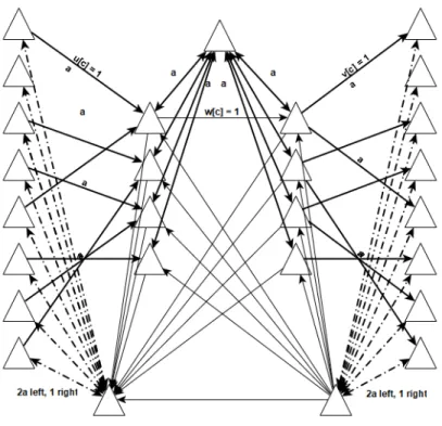
an available leaf ℓ of 𝑇𝑥, and an edge from ℓ to 𝜋(𝑢)0. For each 𝑐 ∈ [𝑑], add a directed edge
Figure 4-2: Sketch of Theorem 4.2.1 construction. Bold edges represent paths, whose labels denote their length.
Stages We proceed in 𝑁2−𝛿 stages, one for each element 𝑤 ∈ 𝑊 . For the current 𝑤, for each coordinate 𝑐 where 𝑤[𝑐] = 1, we add an edge from 𝑟(𝑇𝑐𝑈) to 𝑟(𝑇𝑐𝑉). We then query
the one-way radius or all one-way eccentricities of 𝐺. We will show that if there is a 𝑢 that forms a hitting set with 𝑤, then the one-way radius is most (1 + 𝑜(1)) · 𝑎, and otherwise, the one-way radius is at most (2 + 𝑜(1)) · 𝑎. A (2 − 𝜖)-approximation algorithm for one-way radius or all one-way eccentricities distinguishes between these two cases and can thus detect a hitting set that includes 𝑤 if one exists. If such a hitting set is not detected, we undo the edge additions for the stage and continue to the next 𝑤.
We can modify the stage to be decremental by beginning with a directed matching from {𝑟(𝑇𝑐𝑈) | 𝑐 ∈ [𝑑]} to {𝑟(𝑇𝑐𝑉) | 𝑐 ∈ [𝑑]}, and removing the excess edges each stage.
Analysis
Correctness We first note that all nodes apart from those in 𝑇𝑥and {𝜋(𝑢)𝑖 | 𝑖 ∈ [𝑎], 𝑢 ∈ 𝑈 }
have infinite one-way eccentricity, because they cannot reach 𝑇𝑥.
𝜋(𝑢)𝑎 is of distance at most (1 + 𝑜(1)) · 𝑎 from every other node. For all 𝑢′ ∈ 𝑈, 𝑖 ∈ [𝑎], 𝜋(𝑢)𝑎
can reach 𝜋(𝑢′)𝑖 in at most (1 + 𝑜(1)) · 𝑎 steps, because it may reach all 𝜋(𝑢′)0 in 𝑜(𝑎) steps
via 𝑇𝑥. From the 𝜋(𝑢′)𝑎, 𝜋(𝑢)𝑎 may reach all nodes of the 𝑇𝑐𝑈 in 𝑜(𝑎) additional distance,
because we have discarded all degenerate coordinates. There is some 𝑐 such that 𝑢[𝑐] = 1, so there is a path of length 𝑜(𝑎) from 𝜋(𝑢)𝑎 to some 𝑇𝑐𝑈 and from there to 𝑇𝑦, and from 𝑇𝑦,
𝜋(𝑢)𝑎may reach all nodes of the 𝑇𝑐𝑉 in (1 + 𝑜(1)) · 𝑎 additional distance. Since 𝑢 and 𝑤 define
a hitting set, for all 𝑣 there is a coordinate 𝑐 such that 𝑢[𝑐] = 𝑣[𝑐] = 𝑤[𝑐] = 1. Then for each 𝑣 there is a path from 𝜋(𝑢)𝑎 to 𝑇𝑐𝑈 over an edge between 𝑇𝑢 and 𝑇𝑐𝑈, immediately over an
edge to 𝑇𝑐𝑉, then to 𝑇𝑣 over an edge. Thus in 𝑜(𝑎) steps, 𝜋(𝑢)𝑎 may for all 𝑣 reach 𝜋(𝑣)𝑎,
and therefore may reach all 𝜋(𝑣)𝑖 in at most (1 + 𝑜(1)) · 𝑎. Then 𝑒𝑐𝑐(𝜋(𝑢)𝑎) ≤ (1 + 𝑜(1)) · 𝑎,
which upper-bounds the one-way radius.
Suppose there is no hitting set involving the current 𝑤 and any 𝑢. For all nodes in 𝑇𝑥 and
all nodes 𝜋(𝑢)𝑖 where 𝑖 < 𝑎, the only paths to the nodes 𝑇𝑣 go through some node 𝜋(𝑢′)𝑎.
Therefore the only possible centers of the graph are the nodes 𝜋(𝑢)𝑎. For all 𝑢, there exists
a 𝑣 such that there does not exist a coordinate 𝑐 with 𝑢[𝑐] = 𝑣[𝑐] = 𝑤[𝑐] = 1; in other words, 𝑢, 𝑣, 𝑤 form an orthogonal triple. Fix 𝑢 and 𝑣. Every path between 𝜋(𝑢)𝑎 and 𝜋(𝑣)𝑎 must
visit some node 𝜋(𝑢′ ̸= 𝑢)𝑎 or some node in 𝑇𝑦, which are all of distance (1 + 𝑜(1)) · 𝑎 from
𝜋(𝑢)𝑎. This means that d(𝜋(𝑢)𝑎, 𝜋(𝑣)0) is at least (2 + 𝑜(1)) · 𝑎 for all 𝑢. Since the 𝜋(𝑢)𝑎 are
the only candidates for centers, the one-way radius must be at least (2 + 𝑜(1)) · 𝑎 as well. Only binary trees are added to the base graph, and only a constant number of edges are added to any node, so the maximum degree is bounded by a constant.
Running time 𝐺 is of size ˜𝑂(𝑁𝛿) with ˜𝑂(𝑁𝛿) edges, and we perform ˜𝑂(1) updates
and queries each stage, so the running time argument from subsection 2.3.1 holds.
Theorem 4.2.2. Let 𝜖, 𝜖′, 𝑡 be positive constants. 3HSH implies that there exists no in-cremental or dein-cremental dynamic algorithm for (2 − 𝜖)-approximate radius or max-eccentricities on undirected, unweighted constant-degree graphs with 𝑛 vertices, ˜𝑂(𝑛) edges, and constant maximum degree which has sensitivity 𝜔(log 𝑛), preprocessing time 𝑝(𝑛) = 𝑛𝑡,
Proof of Theorem 4.2.2.
Construction
Initialization Let 𝑎 = 𝜔(log 𝑁 ) and 𝛿 = 1−𝜖𝑡 . We begin with an instance of 3-HS and construct the same graph 𝐺 as in Theorem 4.2.1. Let 𝑁′ = ˜𝑂(𝑁𝛿) be the number of nodes in 𝐺. Let 𝑇𝑧 =
←→
𝑇𝑁′, and add a directed matching from the nodes of 𝐺 to the leaves of 𝑇 𝑧.
Then add an edge from 𝑟(𝑇𝑧) to 𝑟(𝑇𝑥).
Stages We proceed just as in Theorem 4.2.1, except querying for the max-radius or all max-eccentricities rather than the one-way radius or eccentricities.
Analysis
Correctness We first note that all nodes apart from those in 𝑇𝑥and {𝜋(𝑢)𝑖 | 𝑖 ∈ [𝑎], 𝑢 ∈ 𝑈 }
have infinite one-way eccentricity, because they cannot reach 𝑇𝑥.
By the same argument as in Theorem 4.2.1 and noting that all nodes in 𝐺 may reach 𝑇𝑥
in 𝑜(𝑎) distance, if there is a hitting set {𝑢, 𝑤}, then the one-way eccentricity of 𝜋(𝑢)𝑎 is at
most (1 + 𝑜(1)) · 𝑎. Also, every node may reach 𝜋(𝑢)𝑎 in at most (1 + 𝑜(1)) · 𝑎 steps via 𝑇𝑧, 𝑇𝑥,
and 𝜋(𝑢)0. Thus the max-eccentricity of 𝜋(𝑢)𝑎 is at most (1 + 𝑜(1)) · 𝑎, which upper-bounds
the max-radius of 𝐺.
Suppose there is no hitting set involving the current 𝑤 and any 𝑢. Note that max-distance is at least as large as one-way max-distance, by definition. By the same argument as in Theorem 4.2.1 and noting that any path via 𝑇𝑧 from any 𝜋(𝑢)𝑎 to any 𝜋(𝑣)0 is at least
(2 + 𝑜(1)) · 𝑎, any 𝜋(𝑢)𝑎 must have one-way eccentricity of at least (2 + 𝑜(1)) · 𝑎. The nodes of
𝑇𝑥 have one-way distance at least (2 + 𝑜(1)) · 𝑎 to reach any node 𝜋(𝑣)0, and thus so do the
nodes of 𝑇𝑧, because all paths from 𝑇𝑧must pass through 𝑇𝑥. This implies that if any node is
at distance at least (2 + 𝑜(1)) · 𝑎 from some 𝜋(𝑣)0 in the construction of Theorem 4.2.1, then
that node remains at max-distance (2 + 𝑜(1)) · 𝑎 from that node 𝜋(𝑣)0 in this construction.
all 𝜋(𝑣)𝑖 because they were at infinite one-way distance to any node 𝜋(𝑣′)𝑗 for 𝑣′ ̸= 𝑣 in
Theorem 4.2.1, and true for any 𝑇𝑢 because that would imply that there is a hitting set.
However, it may not be true for other nodes if there is some coordinate 𝑐 such that for all 𝑣, 𝑣[𝑐] = 1. We may check if this is the case first, and then see if there is an edge between 𝑟(𝑇𝑐𝑈) and 𝑟(𝑇𝑐𝑉), which would imply that there is in fact a hitting set; otherwise, we may
remove 𝑇𝑐𝑈 and 𝑇𝑐𝑉 from the graph and query again. We would have to repeat this at most
𝑑 = ˜𝑂(1) times, once per coordinate. Now we may observe that if there is no hitting set, all nodes are at least max-distance (2 + 𝑜(1)) · 𝑎 from some node 𝜋(𝑣)0, so the max-radius is at
least (2 + 𝑜(1)) · 𝑎.
Note that we added at most two edges to each node in the construction of Theorem 4.2.1, and all nodes in 𝑇𝑧 have constant degree, so the nodes of this construction have constant
maximum degree as well.
Running time 𝐺 is of size ˜𝑂(𝑁𝛿) with ˜𝑂(𝑁𝛿) edges, and we perform ˜𝑂(1) updates and queries each stage, so the running time argument from subsection 2.3.1 holds.
Here we show the lower bound for min-radius on directed acyclic graphs. We rely heavily on the construction of [3], modifying one of its constructions only slightly.
Theorem 4.2.3. Let 𝜖, 𝜖′, 𝑡 be positive constants. 3HSH implies that there exists no in-cremental or dein-cremental dynamic algorithm for (2 − 𝜖)-approximate radius or min-eccentricities on directed, unweighted acyclic graphs with 𝑛 vertices and ˜𝑂(𝑛) edges, which has sensitivity 𝜔(log 𝑛), preprocessing time 𝑝(𝑛) = 𝑛𝑡, and update time 𝑢(𝑛) and query time 𝑞(𝑛) such that max {𝑢(𝑛), 𝑞(𝑛)} = 𝑛2−𝜖′.
Proof of Theorem 4.2.3.