A comparison of methods for the treatment of uncertainties in the modeling of complex systems

A Comparison of Methods for

the Treatment of Uncertainties in

the Modeling of Complex Systems

by

Isaac Trefz

B.S., Swarthmore College (1994)

Submitted to the Department of Electrical Engineering and Computer Science in partial fulfillment of the requirements for the degree of

Master of Science in Electrical Engineering and Computer Science at the

MASSACHUSETTS INSTITUTE OF TECHNOLOGY May 1998

© Massachusetts Institute of Technology, MCMXCVIII. All rights reserved. The author hereby grants to MIT permission to reproduce and distribute publicly paper and electronic

copies of this thesis document in whole or in part, and to grant others the right to do so.

Author

f/ Department

Certified by.

'I7

of Electrical Engineering and Computer Science May 26, 1998

J. G. Kassakian Professor of Electrical Engineering Primary Thesis Supervisor Certified by_

T. M. Jahns Senior Lecturer of Electrical Engineering Se ondartesis Supgrvisor Accepted by

a DArtnur ~t . mith Chairman, Departmental Committee on Graduate Students JUL

",1P

U

A Comparison of Methods for

the Treatment of Uncertainties in

the Modeling of Complex Systems

by

Isaac Trefz

Submitted to the Department of Electrical Engineering and Computer Science on May 26, 1998 in partial fulfillment of

the requirements for the degree of Master of Science in Electrical Engineering

Abstract

Engineers working on complicated system integration problems in industries such as automotive or aerospace often face a need to understand the impact of uncertainties in their component models, particularly during the early stages of development projects. If such uncertainties are modeled as continuous random variables, system model calculations create the need to evaluate the probability characteristics of functions (i.e., sums, products, etc.) of these random variables. Evaluation of analytical expressions for the resulting probability density functions is often intractable, and even direct numerical evaluations can require excessive computation times using modern computers. As an alternative, there are approximation techniques which hold the prospect of significant reductions in the execution times in return for modest reductions in the accuracy of the resulting density functions.

Methods for approximating mathematical functions of independent random variables are explored based on the assumption that the operand random variables can be modeled as beta distributions. Attention is focused on the arithmetic operations of multiplication, division, and addition of two independent random variables, and the exponentiation of one random variable to a scalar power. Execution times for these approximate evaluation techniques are compared to those using direct numerical calculation and, alternatively, to those using a Monte Carlo approach. Comparisons are made of the accuracies of these alternative approximation techniques to the results of direct numerical calculations for a wide range of beta distribution parameters. These tests indicate that the approximation techniques generally provide good accuracy for addition, multiplication, and exponentiation operations, but the approximation accuracy is poorer for the quotient operation. This limitation is not expected to pose a major impediment to the useful application of these approximations in system model calculations.

Primary Thesis Supervisor: J. G. Kassakian Title: Professor of Electrical Engineering Secondary Thesis Supervisor: T. M. Jahns Title: Senior Lecturer of Electrical Engineering

Dedication

to

my Grandparents

and

my Parents

Acknowledgments

First and foremost I would like to thank Thomas Neff of Daimler-Benz Forschung in Frankfurt a.M. for developing the concept for this work [see 12] and for his supervision and assistance. I hope he finds my work useful when writing his Ph.D. thesis. On the same note, thanks are due to Dr. Michael Kokes and Dr. Hans-Peter Sch6ner of Daimler-Benz for finding the money to pay my way here at MIT. This research would not have been possible without the financial support of Daimler-Benz AG.

Next in line for thanks is Dr. Thomas Jahns. Working closely with a company on the other side of the ocean had its snares, but he managed to work them all out. He also took the time to offer advice whenever I needed it and carefully read several drafts of this thesis.

Professor John Kassakian wasn't afraid to take a chance on me from the beginning. He also let me TA his Power Electronics course and gave me two paid vacations, one to Europe and one to Phoenix. Thanks for all of the good times, John.

Acknowledgments to Khurram Khan Afridi for writing MAESTrO and helping me get my foot in the door with Daimler-Benz. Khurram was basically my mentor here at MIT, and everything I know about wheeling and dealing I learned from him.

Big Thanks to Ankur Garg. MIT is a rough place, and I doubt that I would have survived 6.241, 6.341 and the PWE without her. Her help with this thesis has also proved invaluable. Most importantly though, she is simply a good friend and all-around class act.

The basement of Building 10 may be a hole but Vahe 'Iron Man' Caliskan and James Hockenberry made it a bearable one. Vahe knows everything there is to know about power electronics and is the nicest, most considerate person I've ever met. James and I spent hours on end reminiscing about our alma mater, Swarthmore College, and discussing society's ills. Thanks guys.

Our secretaries here in LEES, Vivian Mizuno, Karin Janson-Strasswimmer, and Sara Wolfson, also deserve thanks for their moral support and willingness to help out with anything and everything.

Contents

1 Introduction 15

1.1 System Analysis Using MAESTrO ... 16

1.2 Objectives and Technical Approach ... ... 18

1.3 O rganization of this Thesis ... ... 19

2 Background 21 2.1 B asic Probability Theory ... ... 21

2.1.1 Expression of Uncertainty as a Random Variable... ... 21

2.1.2 Moments and Central Moments of a Continuous Random Variable ... 22

2.1.3 Characteristic Function of a Continuous Random Variable... 23

2.2 The Generalized Beta Distribution...25

3 Analytical Approximation Methods 31 3.1 Springer's M ethods ... ... 32

3.1.1 Linear Combinations of Two Independent Random Variables ... 32

3.1.2 Multiplication of Two Independent Random Variables ... 34

3.1.3 Exponentiation of One Random Variable ... ... 36

3.1.4 Division and Subtraction of Two Random Variables ... 36

4 Numerical Methods 43

4.1 Analytical Solutions to Functions of Random Variables ... 43

4.1.1 Analytical Convolution of Two Independent Random Variables ... 43

4.1.2 Analytical Exponentiation of One Random Variable... ... 46

4.2 Direct Numerical Approximation to Functions of Random Variables ... 46

4.2.1 Numerical Convolution of Two Independent Random Variables ... 46

4.2.2 Numerical Exponentiation of One Random Variable ... 49

4.3 Monte Carlo Approximation of Functions of Random Variables ... 49

5 Implementation and Experimental Results 51 5.1 Calculation of a Beta Density Function from its Beta Parameters ... 51

5.2 Chi-Squared and Least-Squares Tests ... 54

5.3 Implementation and Comparison of Numerical Methods ... 56

5.3.1 Numerical Convolution of Two Independent Random Variables ... 57

5.3.2 Numerical Exponentiation of One Random Variable ... . 59

5.3.3 Implementation and Exploration of Monte Carlo Methods ... 59

5.4 Implementation and Comparison of Analytical Approximation Methods ... 60

5.4.1 Calculation of Beta Parameters from Central Moments... ... 61

5.4.2 Implementation of Springer's Methods... 61

5.4.3 Implementation of McNichols' Methods ... ... 62

5.4.4 Description of Test Batteries ... 62

5.4.5 Experimental Comparison of Springer's and McNichols' Methods ... 64

5.5 Comparison of Execution Times...71

List of Figures

A simple electrical system that one may analyze using MAESTrO is shown above. This system is comprised of of an alternator, two motor loads, and their associated wiring... 16 Probability density functions that may be used to represent the cost of the alternator

(left), motorl (center), and motor2 (right) of the system shown in Figure 1.1 are show n above ... 17 A probability density function representing uncertainty in the cost of the system of Figure 1.1 is shown above ... 17 The beta density function plotted on the interval [0,1] for various values of a and

3

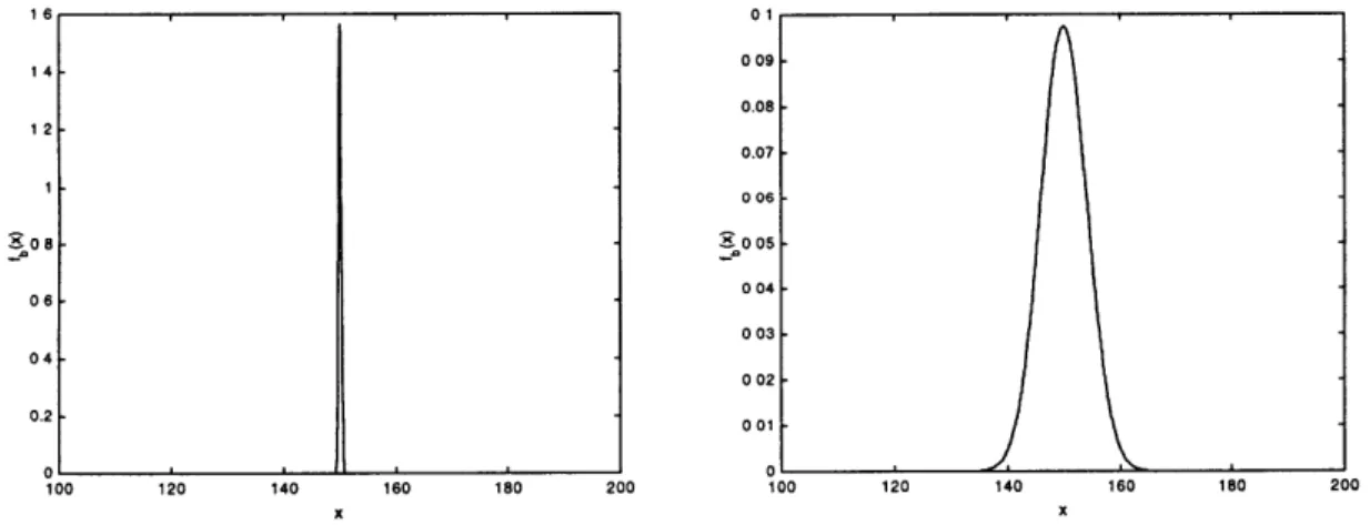
both greater than 1 is shown above. ... ... 26 The beta density function plotted on the interval [0.1] for various values of a and 0 where either a<1 or 3<1 (left) or both a<1 and P<1 (right) is shown above. ... 27 The general method used to approximate a function of two independent beta variables is represented here. The step inside the circle will differ depending on the functional form of the function to be approximated and the approximation method used (i.e. Springer's or M cNichols') ... ... 31 Plots of fb = (x;2 x 104,2 x 104,100,200) (left) and fb = (x;75,75,100,200) (right) are shown above. Note how much sharper the density function on the left is compared to the density function on the right... 53 A flowgraph of the chi-squared routine used to test each all approximation routines is show n above. ... 55 A flowgraph of the least-squares routine used to test each of Springer's and McNichols' approximation routines is shown above ... . 57 Plots of the product of fb(x;2,1,0,1) and fb(x;3,1,0,1) generated using numerical convolution (left) and this same curve superimposed upon fb(x;2,2,0,1) (right) are shown above. The plot on the left shows that the technique yields smooth curves, while the plot on the right shows that accurate curves are yielded through this technique as w ell. ... 58

Figure 5.5: The product of f, = fb(x;2,1,0,1) and f2 = fb(x;3,1,0,1), calculated using the Monte

Carlo method (solid), and the known product g = fb (x;2,2,0,1) (dashed) are plotted above. Comparison with Figure 5.4 shows that the convolution based methods described in the previous section are far superior in terms of the smoothness of the result than the Monte Carlo method described in this section. ... 60 Figure 5.6: Plots of the approximation to the product of fb(x;4_.1,8_{.15,0,1) and fb(x;}9_,9_.3 3_,0,1)

shown on the interval [0,0.6] are shown above for Springer's method (left) and McNichols second order method (right). It can be seen that Springer's method yields the better approximation ... 67 Figure 5.7: Plots of Springer's approximation to the product of fb(x,1.2 4_,3_.8_{1,0,1) and}

fb(x,l.12,4.4 6,0,1) and the numerically generated benchmark density function on the interval [0,0.1] are shown above. In this case, Springer's method yields a result of fb(x,0.5 7,21.70,0.00,1.7 9) and a least-squares metric of 2.06 ... 68 Figure 5.8: Plots of Springer's approximation to the sum of fb(x;9.2 5,2.11,0,1) and fb(x;1.12,4_.3 3_{,0,1) and the numerically generated benchmark density function on the}

interval [0,2] are shown above. In this case, Springer's method yields a result of fb(x;4 9.7 5,4 9.7 5,-0.9 2,2.9 6) and a least-squares metric of 0.0177. ... 68 Figure 5.9: Plots of the approximation to the quotient of fb(x;4.7 4,3.7 5,1,2) and fb(x;8.87,1.36,1,2) on the interval [0.4,1.5] are shown above for the three methods tested. Both McNichols' first and second order approximations are more accurate than Springer's, but it is difficult to discern that from this figure ... 69 Figure 5.10: Plots of Springer's approximation to the quotient of fb(x;8.15,1.5 3_,1,2_{) and}

fb(x;6.4 3,1.4 5,1,2) and the numerically generated benchmark density function on the interval [0.5,1.5] are shown above. In this case, Springer's method yields a result of fb(x;6.10,6.10,0.6 5_,1.3 9_{) and a least-squares value of 0.2151 ... 70}

List of Tables

Table 1.1: Assumptions about the minimum, maximum, and most likely costs of the alternator and motors of the system shown in Figure 1.1 are given above... 17 Table 3.1: The cumulants of Y = p(X, X2,..., X,) as a function of the central moments of

Xj,X2,...,X,, for McNichols' first order approximation (see Equation (3.22)) ... 38

Table 3.2: The cumulants of Y = Tp(X 1, X2,...,X,) as a function of the central moments of

X,X 2,...,X,, for McNichols' second order approximation (see Equation (3.23))... 39

Table 3.3: The cumulants of Y = X1X2 as a function of the central moments of Xj and X2 for

McNichols' first order approximation... ... 40 Table 3.4: The cumulants of Y = XX 2 as a function of the central moments of X, and X2 for

McNichols' second order approximation ... ... 40 Table 3.5: The cumulants of Y = X1/X2 as a function of the central moments of XI and X2 for

M cNichols' first order approxim ation... 41 Table 3.6: The cumulants of Y = XI/X 2 as a function of the central moments of X and X2 for

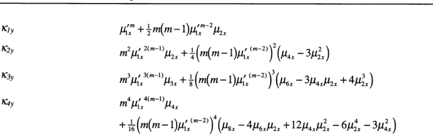
McNichols' second order approximation ... ... 41 Table 3.7: The cumulants of Y = X" as a function of the central moments of X1 for McNichols'

first order approxim ation... ... 42 Table 3.8: The cumulants of Y = X' as a function of the central moments of X, for McNichols'

second order approxim ation ... 42 Table 5.1: The beta parameters and number of tests run for the first battery of random tests on Springer's and McNichols' approximation algorithms are shown above. All of the beta shape parameters, a and P, were produced using a random number generator... 63 Table 5.2: The beta parameters and number of tests run for the second battery of random tests on Springer's and McNichols' approximation algorithms are shown above. All of the beta interval boundries, a and b, were produced using a random number generator.. 64 Table 5.3: The results of the first battery of tests run on Springer's and McNichols'

approximation methods are shown above (see Table 5.1). For each arithmetic operation and approximation method, the number of trials out of one hundred that failed a chi-squared test is given, along with the average over all one hundred trials of

the least-squares test (see Equation (5.11)). Note that McNichols' first and second order methods are identical to Springer's method for the case of addition (see Section 3.2)... ... 65 Table 5.4:The results of the second battery of tests run on Springer's and McNichols'

approximation methods are shown above (see Table 5.2). For each arithmetic operation and approximation method, the number of trials out of one hundred that failed a chi-squared test is given, along with the average over all one hundred trials of the least-squares test (see Equation (5.11)). Note that McNichols' first and second order methods are identical to Springer's method for the case of addition (see Section 3.2)... ... 66 Table 5.5: Execution times in seconds of all of the numerical and analytical methods explored for generating approximations to products, quotients, sums, and powers of independent beta random variables are shown above ... 71

1 Introduction

Enterprises that perform system integration must be able to evaluate system components in early development stages, when more than half of total product costs is determined [3]. Manufacturers of automobiles and trucks are excellent examples of such enterprises. At present almost all development and determination of subsystem costs is done by the suppliers of individual subsystems, but there is a need for the producer of the overall system to plan and coordinate the development of these subsystems. The system integrator must therefore be able to effectively model economic aspects, such as life-cycle costs, and technical aspects, such as electrical losses, of system components. During the early development phase when system alternatives are discussed, not all of the information required for an effective comparison of various system topologies is available. Many of the attributes of various system components can only be represented by estimated values. Nevertheless, important product decisions are made on the basis of these inexact estimates. It is therefore desirable to render visible the uncertainty apparent in all available data and the results of any system analysis before major decisions are made.

One method of modeling uncertainties in component attributes is to use continuous random, or stochastic, variables. Uncertainty in overall system attributes may then be calculated and also represented in the form of continuous random variables. The representation and calculation of system attributes using random variables opens up the possibility of assessing the risks involved with a given project. There are presently several well known mathematical methods for calculating functions of several random variables [see 16]. Unfortunately, many of these methods require long computation times or are not well suited for implementation on a computer [see 2 for an example of this]. When the systems to be modeled are large and results are needed quickly, long computation times and large data structures become a major hindrance. The purpose of this thesis is to investigate methods for efficiently, accurately, and quickly carrying out mathematical operations with random variables, which will lend themselves well to computer implementation and integration into software.

1.1 System Analysis Using MAESTrO

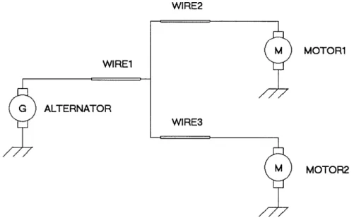
MAESTrO [19] is a software tool specifically designed to analyze alternative electrical system configurations for automobiles and trucks. Specifically, MAESTrO is capable of calculating estimates of the total cost, weight, reliability, and efficiency of an entire electrical system as well as of its generation, storage, distribution, and utilization subsystems. Figure 1.1 shows a simple electrical system that one may analyze using MAESTrO. This system is comprised of an alternator, two motor loads, and their associated wiring. Suppose we wish to calculate the cost of the entire system by adopting the simple cost model assumption that the cost of the total system is equal to the sum of the costs of all six system components. At present, the cost of each component, and thus of the entire system, can only be calculated deterministically in MAESTrO. All of the input parameters describing each component to MAESTrO are scalars, and the cost of the system is therefore output by the software as a scalar. However, this scalar result cannot meaningfully represent the uncertainty present in the cost of the system due to uncertainty present in the parameters used to calculate the costs of each individual component.

As an example, we will now proceed to probabilistically calculate the cost of the system shown below. Suppose that each of the three wires is known to cost $5, and we make the assumptions shown in Table 1.1 about the minimum possible, maximum possible and most likely costs of the other three components.

WIRE2 M MOTOR1 WIRE1 G ALTERNATOR WIRE3

M

MOTOR2

Figure 1.1: A simple electrical system that one may analyze using MAESTrO is shown above. This system is comprised of an alternator, two motor loads, and their associated wiring.

a Alternator Motorl Motor2 $30 $20 $5 $40 $30 $35 $27 $7 Table 1.1: Assumptions about the minimum, maximum, and most likely costs of and motors of the system shown in Figure 1.1 are given above.

the alternator

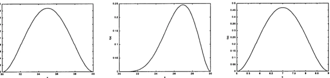
Figure 1.2: Probability density functions that may be used to represent the cost of the alternator (left), motor (center), and motor2 (right) of the system shown in Figure 1.1 are shown above.

014

0.12

Figure 1.3: A probability density function representing Figure 1.1 is shown above.

uncertainty in the cost of the system of

The cost assumptions shown in Table 1.1 can be approximated by the probability density functions shown in Figure 1.2. We can use convolution to add these three density functions to each other and to the total cost of the three wires ($15), to obtain a density function representing the cost of the entire system. This result is shown in Figure 1.3 and yields a great deal of valuable information about the uncertainty inherent in the cost of the entire system. For example,

AS as 03 26 0.2 16 0 1 06 0 1 66 1 1 1.1 .6I

Minimum Cost Maximum Cost Most Likely Cost

it is clear that this cost will not be less than $75, nor exceed $91. The expected value of the cost can also be calculated to be $82.85.

We can also find the probability that the cost of the system will be between two values, x, and x2

by integrating the above distribution over the interval [xjX2]. For example, suppose we have

defined a maximum cost target for our system of $85. We can integrate the above distribution from x = $0 to x = $85 in order to find the probability (77.5%) that we will meet this cost target. Knowing that a system design may meet a desired cost target with a probability of only 77.5% long before the system is about to enter production could prove to be a valuable piece of information at early design stages. Unfortunately, such information cannot be obtained with the current implementation of MAESTrO.

The goal of this thesis is to explore means of extending MAESTrO to allow users to define component parameters as probability density functions, as opposed to simple scalars. From these density functions representing component parameters, we wish to compute probability density functions representing subsystem and system attributes such as cost, weight, reliability, and efficiency. In order to be able to do so, we must find fast and effective methods to compute mathematical functions of random variables.

1.2 Objectives and Technical Approach

The overall objective of this thesis is to investigate methods of approximating probability densities of functions of independent random variables for the purpose of using in the MAESTrO software tool. Stated mathematically, if X1, X2,.... X, are independent real random variables

with density functions f,(x),f2(x),...,fn(x) and Y= (X,,X2,... X,), where p is any arbitrary

real function, we would like to find a reasonable approximation to the probability density function of the random variable Y, g(y), using the density functions of X1, X2,..., X,.

While it is theoretically possible in many instances to find a closed-form analytical expression for g(y), this expression can be very complicated, difficult to derive, and impossible to evaluate on a computer. It is therefore desirable to find an acceptably good approximation to g(y) using simple numerical algorithms that would require a fraction of the computational time and resources of their analytical counterpart. This thesis will compare methods for approximating the density function, g, of the function of independent random variables, (p.

The technical approach adopted in this work is to investigate the following three methods for performing calculations with random variables and to compare them with regard to their relative speed and accuracy:

1. Direct numerical calculation of g(y) based on analytical expressions 2. Monte Carlo approximation to g(y)

3. Analytical approximation to g(y) using the moments or cumulants of X , X,,..., X

The mathematical operations that will be investigated are products, quotients, and linear combinations of two independent random variables, and exponentiation of one random variable to a scalar power. While analytic expressions for all of these operations exist, they typically involve convolution integrals that are difficult or impossible to evaluate analytically. These expressions may however be used as a basis to directly generate numerical approximations to g(y).

A Monte Carlo approach can serve as an alternative to direct numerical approximation of analytic expressions and has the advantage that it does not require there to be an analytic expression available for the density function being approximated. This approach is considerably more complicated than direct numerical calculation but can in some cases lead to improvements in speed and accuracy.

Although direct numerical calculation and Monte Carlo calculation of functions of independent random variables may require less time and computational resources than a direct analytical approach, the computational savings that these methods offer may still not be enough if we have models that require many stochastic calculations or require storage of many stochastic variables. Fortunately, methods are available to approximate the density function of Y = q(X,,X2,..., X,) using simple calculations and the moments of X,, X2,..., X. Three of these methods, one developed by M. Springer [16] and two developed by G. McNichols [11] can offer significant savings in computation time and resources over direct numerical calculation or a Monte Carlo approach.

1.3 Organization of this Thesis

As mentioned in the previous section, this thesis will explore three methods for approximating the density function, g(y), of the random variable Y = p(X,X 2, ...,X), where X,,X2,...,X, are independent random variables and (p is a real function. Chapter 2 begins with an introduction to

the basic concepts of probability theory that are necessary to the derivation of the analytical approximation methods of Springer and McNichols, and concludes with a description of the generalized beta distribution which is used for all calculations in this thesis.

Chapter 3 develops the analytical approximation methods that will be used to approximate the density function of Y, g(y). The general method for approximating a function of beta distributions with a beta distribution is introduced. Subsequently, Springer's and McNichols' methods, which are used to calculate the moments of the approximating beta distribution, are developed out of the theory of Chapter 2.

Chapters 4 develops the numerical and Monte Carlo methods that will be used to approximate the density function of Y, g(y). Analytical expressions for the density functions of products, quotients, sums, and differences of two independent random variables, as well as exponentiation of one random variable to a scalar power, are derived, and algorithms are developed to generate numerical approximations based on these analytical expressions.

Chapter 5 begins with a discussion of implementation issues surrounding the direct numerical and Monte Carlo algorithms of Chapter 4 and compares the two approximation methods on the basis of the smoothness and accuracy of the approximations they generate. Implementation issues surrounding the analytical approximation methods of Chapter 3 are then discussed. Two batteries of tests are used to compare Springer's and McNichols' methods, and their results are presented. The chapter concludes with a comparison of the execution times of all the

approximation methods under study.

Chapter 6 summarizes the results of Chapter 5 in the context of the extension of MAESTrO to perform calculations with random variables. The conclusion is reached that while direct numerical techniques are still too slow for software implementation, Springer's approximation techniques hold promise for the addition, multiplication, and exponentiation operations. The

approximation accuracy for the quotient operation is found to be poorer. However, this limitation is not expected to pose a major impediment to the useful application of these

2 Background

Basic probability theory and the beta distribution are fundamental to the derivation of the analytic and numeric methods that are the subject of exploration of this thesis. Section 2.1 introduces the concepts of a random variable, the moments and central moments of a random variable, and the characteristic function of a random variable. These basic ideas are then applied to generalized beta random variables in Section 2.2 in order to show that a beta random variable can be completely and uniquely characterized by its first four moments.

2.1 Basic Probability Theory

This section introduces basic concepts of probability theory necessary to develop the numerical approximation methods described in Chapter 3. The section begins with the definition of a random variable and its associated distribution and probability density functions. Expressions for calculating the moments of a random variable from its density function and its first four central moments from its moments are then presented. Finally, it is shown through the use of the characteristic function that a reasonable approximation to the density function of a random variable may be obtained from the random variable's moments.

2.1.1 Expression of Uncertainty as a Random Variable

An uncertain quantity can be modeled as a random variable. Probability theory differentiates between discrete and continuous random variables. A discrete random variable may only assume a finite or countable number of values, whereas a continuous random variable may assume an infinite number of values within the interval upon which it is defined [5]. Random variables shall be denoted henceforth by uppercase letters and the values that they may assume by lowercase letters.

Every random variable has a non-negative, monotonically non-decreasing distribution function, F(x), associated with it defined as:

where F(-o) = 0 and F(o) = 1. If F(x) is continuous and everywhere differentiable, we may define the probability density function of a random variable, f(x) = dF(x)/dx.

density function has the following properties:

f(x) O0 P(x, < X < x2) = 2f(x)dx

f

2.1.2 Moments and Central Moments of a Continuous Random Variable

The rth_{moment of a random variable about zero is given by [9]:}

u

_f(x)dx

The first moment about zero of a random variable, Mi , is called its mean or expected value.

We may also define the set of moments about the mean of a random variable and call these the central moments. The rth central moment of a random variable is therefore given by:

yr = E((X - ')r) = (x- ') f (x)dx (2.4)

The following is true of the first and second central moments:

A2 = E(X - ') = E(X) - '= 0

p2 = E(X - /A 2= E(X2) - 1 2= /k4_g2

(2.5a) (2.5b)

The second central moment of a random variable is also known as the variance and is often written as o .

Similarly, the third and fourth central moments of a random variable may be expressed in terms of the moments:

13 = - 34' + 2' 3 _(2.6a)

, = lu - 4u₃'U'+ 64'2 - 3p'4 _(2.6b)

2.1.3 Characteristic Function of a Continuous Random Variable

The expectation of the random variable eitx _{considered as a function of the real variable t is}

known as the characteristic function of X [13]. The characteristic function of a random variable X has many important properties and is crucial in establishing a connection between the moments of a distribution and the distribution itself. A random variable's distribution function is completely determined by its characteristic function, and the characteristic function of a random variable may be expressed as a function of the moments. Thus, the distribution function of a random variable may be completely specified through moments. As this fact will form the basis for all of the analytic approximation methods developed in Chapter 3, a further exploration of the characteristic function is necessary.

The characteristic function of a real random variable X is given by [13]:

O(t) = E(et") =

Jet

Since

Ieitx

1 itx

f(x) = e-i'~(t)dt (2.8)

Given that the characteristic function is differentiable, its rth derivative is given by:

dro- _{ir x' ei f (x)dx}

(2.9) dth Equation (2.3), we obtain:

,L= di i =O (2.10)

Given that a random variable has moments up to order n, we may express its characteristic function as a Maclaurin series:

(t) = 1+ I ' tr +R,(t) (2.11)

r=1 r!

However, as n -> oo, the residual term, Rn, converges to 0:

lim R,(t) = lim ' n+l tn"+ _{=0 (2.12)}

n-+- -- (n +1)!

Thus, the characteristic function may be expressed as an infinite series of the moments:

0(t) = lim 1 + Ir-t (2.13)

We have shown that if an infinite number of the moments of a random variable exist and are known, then its characteristic function, and thereby its distribution and density functions, may be completely determined. However, in almost all practical cases not all of the moments of a given random variable are available. One can however approximate the density function of a random variable by using a finite number of moments.

Suppose we wish to approximate the density function of a random variable using the following finite power series [9]:

f Y a xi (2.14)

j=0

Iff is defined on the closed interval [a,b], the coefficients of ar may be determined by the method of least-squares. In order to do so, the following expression must be minimized:

g =

f

a j=0

Differentiating with respect to the coefficient ar, where r is any integer on the interval [O,n], and setting the result to 0 yields:

- 2 f- ajx xdx = , r = O,..., n (2.16a)

a j=0 )

b b n

Sxrfdx = = f ajxJ+dx, r=O,...,n (2.16b)

a a ji=

If two distributions have equal moments up to an arbitrary order n, then they will have the same least-squares approximation, as the coefficients aj are determined by the moments. This result opens up the possibility of approximating a function of one or more random variables by its moments. According to Kendall and Stuart, the first four moments of a distribution function are sufficient to yield a reasonably good approximation to that distribution function, given that we have some information about the type of the resulting distribution function. In the following section we will describe a distribution function that is uniquely specified by its first four moments.

2.2 The Generalized Beta Distribution

The generalized beta distribution [15] is able to represent the sort of uncertainties that arise in practical industrial applications quite well, since it is defined over a finite interval (as opposed to the Gaussian distribution) and provides a close approximation to a large number of other types of distribution functions.

The generalized beta distribution is defined uniquely by four parameters, a, /, a, and b, and its density function is given by the following relationship:

1 F( /3) (xaa) (b x)l (2.17)

f(x; , fl, a,b) =

(b

where a 5 x 5 b and a, p > 0. The F-function is defined as:

(2.18)

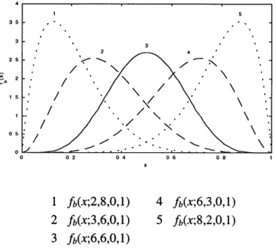
The beta distribution is useful for representing a wide range of distribution functions over the finite interval a 5 x 5 b. The parameters a and / are both shape parameters. When a and P are both greater than 1 (see Figure 2.1), the distribution will have only one peak at:

a(P - 1)+ b(a - 1)

Xpeak = a,)+b(a or a> 1 and P > 1

a+P-2 (2.19)

When a and P are both less than 1, the function assumes a U-shape. When a 2 1 and P < 1 it is J-shaped, and when P 2 1 and a < 1 the function takes the shape of an inverse J (see Figure 2.2). The function becomes the uniform distribution when a =

/

4 1 5 35 -3 - ₃ 2 4 25 0 5 o / 1 fb(x;2,8,0,1) 4 fb(x;6,3,0,1) 2 fb(x;3,6,0,1) 5 fb(x;8,2,0,1) 3 fb(x;6,6,0,1)

Figure 2.1: The beta density function plotted on both greater than 1 is shown above.

the interval [0,1] for various values of a and 03 F(x) = (x- 1)!= e-ttX-'dt

1 fb(x;0.25,4,0,1) fb(x;0.5,0.5,0,1) 2 fb(x;4,0.25,0,1)

Figure 2.2: The beta density function plotted on the interval [0.1] for various values of a and

3

In order to be able to approximate a distribution whose first four moments are known with a beta distribution, it is necessary to establish a relationship between the first four moments of a beta distribution and its four beta parameters. McNichols [11] has calculated the mean, second, third, and fourth central moments of the generalized beta distribution as a function of the beta parameters:

'=a ++(b-a) a+P (2.20a)

112 = 2 ((= _{(b-a)2)( + )2} (2.20b)

p3 =

(b-a)

la

y4= (b - a) 4 _(2.20d)

(a + p + 3)(a + p + 2)(a + p + 1)(a + )4

It is also possible to calculate the four beta parameters from the mean, variance, third and fourth central moments. The beta distribution shape parameters, a and P, may be recovered from the mean and first three central moments using the following relations [8]:

6(P2 -

3,

r = (2.21)

6+ 33 - 22

a, = rlr 1±(r+2)I A(r+ 2)2tA +16(r+ 1) (2.22)

where

S3

If y3 > 0, then

P

/3.

Once the shape factors a and

3

(a +

p

c=

j1

a

a = c ('- (2.24b)

b = a + c (2.24c)

This shows that a beta distribution is uniquely and completely characterized by its first four moments. The above result allows us to attempt to approximate a function of one or more independent beta random variables by simply calculating the first four moments of the result and fitting the corresponding beta distribution to this result. There is however no guarantee that a

beta distribution will serve as a good approximation to a function of independent beta distributions, since products, linear combinations, quotients, and powers of independent beta distributions are not in general beta distributions. It is experimentally tested in Chapter 5 whether products, sums, quotients, and powers of independent beta distributions can be well approximated by beta distributions.

3 Analytical Approximation Methods

This chapter addresses the problem of approximating linear combinations, products, quotients, and powers of independent beta variates. The methods described are intended to greatly simplify and quicken the process of performing mathematical operations with beta variates by avoiding having to perform convolution or Monte Carlo analysis (see Chapter 4). Each method enables calculation of the moments of a function of two or more random variables given only the moments of these random variables. Two separate methods are described for multiplication, division and exponentiation and one method for linear combinations of random variables. Section 3.1 describes methods developed by Springer in 1978 (see [16]), and Section 3.2 describes methods developed by McNichols in 1976 (see [11]).

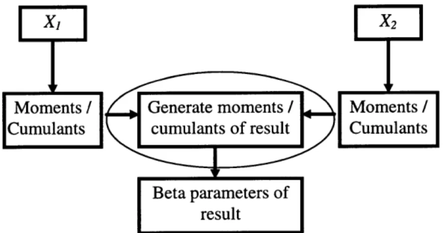
Figure 3.1 shows the general method that is used to calculate the moments of two independent beta variables. The first step is to calculate the required moments or cumulants (see Section 3.1 for a treatment of cumulants) of the random variables X1 and X2. Once these have been

calculated, either one of Springer's or McNichols' methods is used to calculate the first four moments or cumulants of the resulting distribution. These can then be used to calculate the four beta parameters of the resulting approximation using the relations given in Section 2.2.

Figure 3.1: The general method used to approximate a function of two independent beta variables is represented here. The step inside the circle will differ depending on the functional form of the function to be approximated and the approximation method used (i.e. Springer's or McNichols').

3.1 Springer's Methods

In [16] Springer develops relations for exactly calculating the moments of a random variable that is a linear combination, product, or quotient of two other independent random variables as well as the moments of a random variable raised to a scalar power (exponentiation). As described in Section 3.1.1, the expression for the moments of a linear combination of independent random variables relies on a set of descriptive constants known as cumulants, which are derived from the logarithm of the characteristic function described in Section 2.1.3. Mellin transform theory is employed in Sections 3.1.2 and 3.1.3 to derive expressions for the moments of the product of two independent random variables and the moments of one random variable raised to a scalar power. Finally, expressions for the moments of the quotient and difference of two random variables are derived in Section 3.1.4 as special cases of multiplication and exponentiation, and linear combinations respectively.

3.1.1 Linear Combinations of Two Independent Random Variables

In order to calculate the moments of the random variable Y = a + bX; + cX₂ we will require a set of descriptive constants other than the moments, as the moments of Y cannot be readily calculated from the moments of X and X₂. This set of descriptive constants of a random variable are called cumulants and are derived using the characteristic function of a real random variable, which was described in Section 2.1.3. The characteristic function of the random variable Y = X1 + X2, (p(t), is simply the product of the characteristic functions, <pl(t) and <p2(t), of the

two independent random variables, X1 and X2, [13]:

(t)= E(e't ) = E(eit( x+x2)) = E(e'txl e' 2 _(3.1)

= E(eit' )E(eitX2 ) = (t)2 t)

By taking the natural logarithm of the characteristic function, an additive relationship can be established. It is therefore expedient to define the following function, known as the cumulant

generating function:

V(t) = ln(O(t)) (3.2)

The cumulant generating function of Y, ly(t), can now be expressed as the sum of the cumulant generating functions of X, and X2, fl (t) and y2(t):

V(t) = l (t) + V2(t)

Similar to the way the moments were defined in terms of the characteristic function, we define the rthcumulant of Y in terms of the rth derivative of Vy(t), the cumulant generating function of Y:

r, = i-r'_{dtr o} (3.4)

Using the above relations, one can derive expressions for the cumulants of Y in terms of the moments of Y. This is done by Kendall and Stuart [9] for the cumulants up to order 10. For the purpose of this thesis only the first four cumulants of any given random variable will be needed. These are given in terms of the moments by:

K, =

4

x3 = 3pI+ 414'- 212 42 -6

K4 = 4 - 4p''- 3 42 +12 p2; 2 - 6p'4

(3.5)

Manipulation of the above cumulants:

set of equations yields expressions for the moments in terms of the

g '=IK P4 = K2+ K 2 (3 6) p ' = K3 + 31c2K + K 13 4 = K4 + 4K3 1 + 3K22 + 6K2K2 + K14

The variance, third, and fourth central moments can also be expressed in terms of the cumulants:

A12 = (2 = K2

= C3 (3.7

)

14 = K4 + 3K22

It is now possible to derive expressions for the first four cumulants of Y = a + bXj + cX2 in terms

of a, b, c, and the cumulants of X1and X2. The characteristic function of Y is given by [12]:

(3.3)

O(t) = E(ei') = E(exp{it(a + bX, + cX2))= eita ((tb) - (tc))

By taking the natural logarithm of t(t) we obtain its cumulant generating function:

Wy (t) = ita + 01(tb) + 2(tc) -U (3.9)

Employing Equation (3.4), we find" the following expressions for the first four cumulants of Y [11]: a- b-x, c-K X2 K2y 0 b2 12x C2 2 = + + 3 K'3y 0 b3 .3xK .3 3x₂ f'4y. -0

b4

3.1.2 Multiplication of Two Independent Random Variables

It is necessary to use the Mellin Transform to derive an expression for the moments of Y = X1X2

from the moments of X and X2. If the integral:

xk-1 f (x)ldx , where x 2 0 (3.11)

converges for x and k real, then the Mellin transform off(x) exists and is given by [16]:

M (f(x)) = xS-'f (x)dx (3.12)

where s is complex. f(x) can be recovered from Ms(f(x)) using the Mellin inversion integral:

(3.13)

C+o

f

c-loo

where c is a real constant. The Mellin Transform of the density function of Y = X X2 is given

by:

M,(g(y)) = E(YS-')= E((XX 2)s

- '_{) (3.14)}

If X1 and X2 are independent, we may express the probability of the intersection of the events

X1c A and X2 eB as [13]: P{(X, e A)(X2 e B)} = P((X, X2) Ax B) = fff(xP,x2)dxdx2 (3.15) AxB

=

f

Thus if X1 and X2 are independent, the Mellin Transform of their product is given by the product

of their Mellin Transforms:

E((X1X2 )-1) = E(Xs-')E(X-'1)= M,(f,(x,))M,(

f

From the definition of the Mellin transform given above and the definition of the rh moment given in (2.3), it is clear that:

I' = E(X')= Mr+,(f (x)), where x 2 0 (3.17)

Combining Equations (3.16) and (3.17), we find that the rth moment of Y= XX2 is given by:

ly = Px, 'x 2 (3.18)

Fan [4] compared the first ten moments of products of several beta distributions obtained using the above approximation with the moments of products of the same beta distributions obtained analytically using Mellin transform methods and showed that the above approximation yields very good results.

3.1.3 Exponentiation of One Random Variable

The Mellin Transform is required to derive a general expression for the moments of the random variable Y = X. If Y has density function g(y) and X has density function fix), then the Mellin transform of Y is given by [16]:

(3.19)

M,(g(y)) = E(YS-')= E(( X) - Xm(-) f (x)dx

0

From Equation (3.17), equation:

the rhmoment of Y (if it exists) is given by letting s = r + 1 in the above

(3.20)

= E(Y'r) = xmrf (x)dx =p'm.r)x

0

Thus, the rth moment of Y = X is given by the m -r moment of X.

If the density function of X is defined on the closed interval [a,b], and b > a > 0, then the above integral will converge for all m and r, and we may write:

py = E(yr) = E(X mr) = m.r)x (3.21)

3.1.4 Division and Subtraction of Two Random Variables

Both division and subtraction can be accomplished using the methods described in the previous three sections of this chapter. To find the moments of Y = X / X2 = X1(X2)-1 we can use

Equations (3.18) and (3.20):

(3.22)

P =y = Yrx -r)X₂

Similarly, the cumulants of Y = X, - X2 = X, + (-1)X 2can be found from Equation (3.10):

Kr = KrxI -Krx2_{ly rx r}

3.2 McNichols' Methods

Using Springer's methods, exact expressions were found for the moments of a random variable Y which is a function of one or more other random variables. In [ 11] McNichols develops first and second order methods for approximating the moments of a random variable Y = Tq(X, X₂,..., X,), where T is any arbitrary function of real random variables. His first order

method relies on finding a linear approximation to the function T, while his second order method depends on finding a quadratic approximation thereof.

If a function Y =

qp(X

be approximated about the point X' = (XI°,X2 ,...,Xn) by a first order polynomial Y as follows:

Y = p(X,, X2,..., X,)= p(Xo +I (X) (Xi - Xo) (3.24)

i=1 dXi x=xo

Similarly, if a function Y = (X,, X2,..., X,) has continuous first and second partial derivatives

for each Xi, then it can be approximated about the point XO = (XIoX 20, ....X,,o) by a second order

polynomial Y2 as follows: Y2 = (X,, X2... X)=(X)+ (X) (X X) ij Xo n 82p(X) (Xi X;o) 2 i=1 d X=XO 2

Since the density of a random variable will tend to be concentrated around its mean, the highest degree of accuracy will usually be obtained by applying the above approximations about the point X0 = ( 'X' ,14X . ) [13]. If Y is a function of one or more random variables whose

density is not concentrated about the mean (such as a beta variate with a and

13

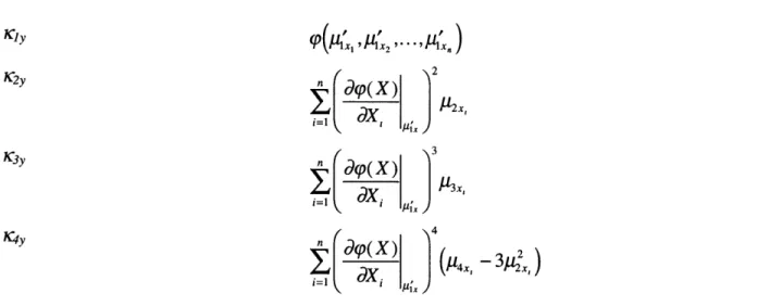
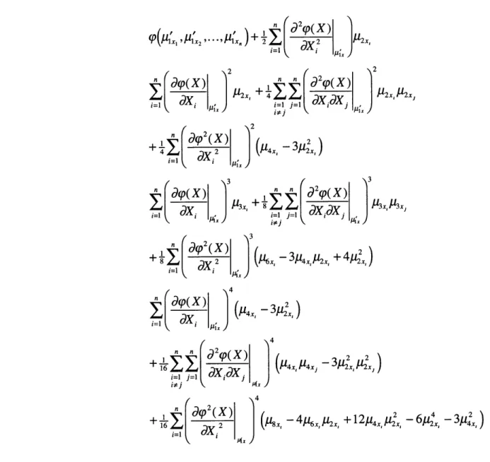
McNichols has applied (3.24) and (3.25) about the point X ° = ( ,₁ "'2 ,.--,/n ) in order to find approximations to the cumulants of Y = 9(X) as functions of the central moments of X [ 11]. His results are summarized in Table 3.1 and Table 3.2. For the case of linear combinations of independent random variables, McNichols' first and second order methods reduce to Springer's method (see Equation (3.10)). Expressions for the first four cumulants of the product and quotient of two independent random variables and those of a random variable raised to a scalar power have been derived for McNichols' first and second order methods and the results summarized in Table 3.3 through Table 3.8.

Cumulant of Y _{Expression in terms of the central moments of Xj,X 2,...,X,}

cly

3C~y

n dg(X) ₃

n d p (

_dX

I

_x

Table 3.1: The cumulants of Y=

9(X

,

Cumulant of Y Expression in terms of the central moments of X1,X2,..

a2<p(x))

d

dp(X)

x

_MI

2

d£

a(x)

d

)J2

dXidX,

₃

q((X)

_{1 1 d}

d9(

d

_p(x)

dxidx.

- 322x, )

Table 3.2: The cumulants of Y = <p(Xl, X2,..., X,) as a function of the central moments of

XI,X2,...,X,, for McNichols' second order approximation (see Equation (3.23))

Kly

IC₂y

K3y

Expression in terms of the central moments of X;,X2,..., X,, Cumulant of Y

JU2X,

Expression in terms of the central moments of X, and X2

ly PX _{PX 2} +

2Y +A xU2 2X,

C3y

Ax

Sx(2 - 32

)

Table 3.3: The cumulants of Y = XIX2 as a function of the central moments of X, and X2 for

McNichols' first order approximation

Cumulant of Y = X1X2 Expression in terms of the central moments of X, and X2

lly PXl t x₂ 12 *2 1 C2y _x I ll2x2 "- + "XI P .Lx2x2 C₃y A3X2 + Ix2 ₃ X" + 13Xl 4 3X2 y 4x2 -

32

Table 3.4: The cumulants of Y = XX 2 as a function of the central moments of X, and X2 for

McNichols' second order approximation Cumulant of Y = X1X2

Cumulant of Y = Expression in terms of the central moments of X1 and X2 Kly 'C₂y K3y K4y tLx,

/'2

x2

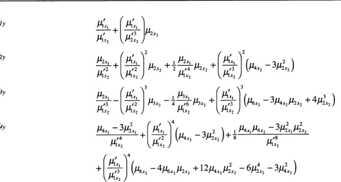
A X2

Table 3.5: The cumulants of Y = X1/X2 as a function of the central moments of X, and X2 for

McNichols' first order approximation

Cumulant of Y = Xs/X2 Expression in terms of the central moments of X1and X2

f

tUx,

, ,

-73

t2l

K

.x.

lA

-x 4

-

3

)

X

12

Table 3.6: The cumulants of Y = X1/X2 as a function of the central moments of X1 and X2 for

McNichols' second order approximation

Cly

14x₁ - 3p2x1 '4 AX ₂

-

344x2

+4

Cumulant of Y = Expression in terms of the central moments of X

2y 0m2 tx2(m-1) x

3 x3(m-1) ,x

/14y m4 4(m-1) 4 -- 32x)

Table 3.7: The cumulants of Y = Xm as a function of the central moments of X1 for McNichols' first order approximation

Cumulant of Y = Xm _{Expression in terms of the central moments of X}

gly

p1m

4

Table 3.8: The cumulants of Y = X as a function of the central moments of X, for McNichols' second order approximation

4 Numerical Methods

This chapter explores methods for finding numerical approximations to the density functions of the sums, differences, products, quotients, and powers of random variables. Given Y = Tp(X, X2) , or Y = p(X) the result of all of the methods described is to generate the vectors g

and y, which represent g(y), the density function of Y, and y sampled at n points. Section 4.1 introduces the Fourier and Mellin convolution integrals associated with addition, subtraction, multiplication, and division of two independent random variables as well an analytic expression for the density function of a random variable raised to a scalar power. Algorithms to find numerical approximations to these analytical expressions are developed in Section 4.2. Finally, Monte Carlo methods are developed in Section 4.3 to determine approximations to g and y for any arbitrary function p.

4.1 Analytical Solutions to Functions of Random Variables

Although this thesis intentionally avoids analytic solution of expressions associated with functions of independent random variables, these expressions form the basis of the numerical methods for finding numerical approximations to sums, differences, products, quotients and powers of random variables described in Section 4.2. The convolution integrals associated with sums, differences, products, and quotients of two random variables are therefore derived in Section 4.1.1, and an expression for the density function of one random variable raised to a scalar power is introduced in Section 4.1.2.

4.1.1 Analytical Convolution of Two Independent Random Variables

Springer [16] gives analytic expressions in the form of convolution integrals for products, sums, quotients, and differences of two independent random variables.

In the case of Y = X1 + X2 the density function of Y, g(y), as a function of the density functions of

g(y)= f(y -x 2). f 2(x 2)dx2

In order to derive this result let:

X1 = y- x₂

X₂ = X2

Since X1and X2are independent, their joint probability element is given by:

(4.1)

(4.2)

(4.3)

f(x, x2)ddx,d2= f(x )f(x2

)dxd

Using (4.2), this becomes:

g(y, x2)dx2dy = f(y - x2)f 2(x 2)Jdx2dy (4.4)

Where J is the Jacobian of the transformation given in (4.2):

1 1

dx dx

J x2 2

dy dx2 _(4.5)

0 1

The variable x2 can be integrated out of (4.4) to yield the density function of Y = X, + X2, given

in (4.1).

Employing the above method and the following transformation:

x1 = y + x2

X₂ = X2

the convolution integral Y = X1 - X2is found to be:

g(y)= f(y + x 2). f 2(x 2)dx2

In the case of Y = XX2, the transformation:

y

X1

-x

2

X₂ X2

yields the Mellin integral for the product of two random variables:

g(y)= f () f(X)dX22

-- X2 2

Finally, the transformation:

x1 = yx₂

X₂ = X2

yields the Mellin integral for the random variable Y = X X₂

g(y)= x2f (yx2) f 2(x2)dx2 (4.11)

The integrals given in Equations (4.1) and (4.7) may be solved using Laplace transform methods and the integrals given in Equations (4.9) and (4.11) using Mellin transform methods. Unfortunately, these analytic solutions can be very difficult to compute and do not lend themselves well to implementation on a computer. Dennis [2] finds an analytic expression for the product of three beta variables using Mellin transform methods, which contains 23 terms and still only serves as an approximation to the actual solution.

(4.7)

(4.8)

(4.9)