HAL Id: hal-01188336
https://hal.archives-ouvertes.fr/hal-01188336
Submitted on 28 Aug 2015
HAL is a multi-disciplinary open access
archive for the deposit and dissemination of
sci-entific research documents, whether they are
pub-lished or not. The documents may come from
teaching and research institutions in France or
abroad, or from public or private research centers.
L’archive ouverte pluridisciplinaire HAL, est
destinée au dépôt et à la diffusion de documents
scientifiques de niveau recherche, publiés ou non,
émanant des établissements d’enseignement et de
recherche français ou étrangers, des laboratoires
publics ou privés.
A bijection for plane graphs and its applications
Olivier Bernardi, Gwendal Collet, Eric Fusy
To cite this version:
Olivier Bernardi, Gwendal Collet, Eric Fusy. A bijection for plane graphs and its applications.
ANALCO’14, Jan 2014, Portland, United States. �10.1137/1.9781611973204.5�. �hal-01188336�
A bijection for plane graphs and its applications
Olivier Bernardi
∗Gwendal Collet
†Eric Fusy
´
‡Abstract
This paper is concerned with the counting and random sampling of plane graphs (simple planar graphs embed-ded in the plane). Our main result is a bijection between the class of plane graphs with triangular outer face, and a class of oriented binary trees. The number of edges and vertices of the plane graph can be tracked through the bijection. Consequently, we obtain counting for-mulas and an efficient random sampling algorithm for rooted plane graphs (with arbitrary outer face) accord-ing to the number of edges and vertices. We also obtain a bijective link, via a bijection of Bona, between rooted plane graphs and 1342-avoiding permutations.
1 Introduction
A planar graph is a graph that can be embedded in the plane (drawn in the plane without edge crossing). A
pla-nar map is an embedding of a connected plapla-nar graph
considered up to deformation. The enumeration of pla-nar maps has been the subject of intense study since the seminal work of Tutte in the 60’s [20] showing that many families of planar maps have beautiful counting formu-las. Starting with the work of Cori and Vauquelin [10] and then Schaeffer [18, 19], bijective constructions have been discovered that provide more transparent proofs of such formulas. The enumeration of planar graphs has also been the focus of a lot of efforts, culminating with the asymptotic counting formulas obtained by Gim´enez and Noy [16].
In this paper we focus on simple planar maps (planar maps without loops nor multiple edges), which are also called plane graphs. This family of planar maps has, quite surprisingly, not been considered until fairly recently. This is probably due to the fact that loops and multiple edges are typically allowed in studies about planar maps, whereas they are usually forbidden in studies about planar graphs. At any rate, the first result about plane graphs was an exact algebraic expression
∗Brandeis University, Dept. Math., Waltham, MA, USA.
†Laboratoire d’informatique de l’ ´Ecole Polytechnique, 91128
Palaiseau, France. [email protected]
‡Laboratoire d’informatique de l’ ´Ecole Polytechnique, 91128
Palaiseau, France. [email protected].
given in [3] (using a non-bijective substitution approach) for the generating function M (z) of rooted plane graphs counted by the number of edges (a planar map is said rooted if it has a marked directed edge with the outer face on its right). Such generating functions expressions can be given in several forms; and recently Marc Noy [17] found a nice simplified form for M (z):
(1.1) M (z) = zB(z)
1− zB(z),
where B(z) = 1+∑n≥1(n+2)(n+1)3·2n−1 (2nn)znis the generat-ing function of rooted bipartite maps counted by edges (including the one-vertex map). By a classical construc-tion, rooted bipartite maps are in bijection with rooted
eulerian triangulations (an eulerian triangulation is a
planar map with triangular faces of two types, dark or light, such that the outer face is dark and each edge is incident to both a light and a dark face); and each edge of the bipartite map corresponds to a dark face of the associated eulerian triangulation. Thus B(z) is also the generating function of rooted eulerian triangulations counted by dark faces.
The identity (1.1) can be reformulated by intro-ducing the generating function C(z) of outer-triangular
plane graphs (plane graphs such that the outer face is
a triangle) counted by edges. Indeed, as explained in Section 3.1, it is easy to see that
M (z) = z(1 + C(z)/z 2) 1− z(1 + C(z)/z2). Hence (1.1) is equivalent to (1.2) C(z) = z 2(B(z)− 1) = ∑n≥1 3·2n−1 (n+2)(n+1) (2n n ) zn+2.
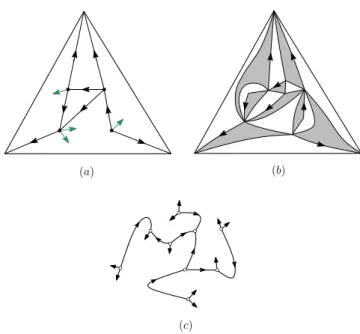
We will prove this identity (and a refinement of it taking into account the number of vertices), by giving a bijec-tion between outer-triangular plane graphs with n + 2 edges and eulerian triangulation with n dark triangles, followed by a bijection between eulerian triangulation with n dark triangles and some oriented plane trees. More precisely, we define an oriented binary tree as a plane tree with vertices of degree 1 (called leaves)
(a) (b)
(c)
Figure 1: (a) An outer-triangular plane graph with 11 edges and 5 inner faces, endowed with its canonical orientation, (b) the corresponding eulerian triangulation with 9 dark faces (including the outer one) endowed with its canonical orientation, and (c) the corresponding oriented binary tree with 11 leaves and 5 sources.
or 3 (called inner nodes), where edges incident to leaves (called legs) are oriented toward the leaf and other edges (called inner edges) are oriented arbitrarily. An inner node whose 3 incident edges are all outgoing is called a
source. We can now state our main result.
Theorem 1.1. For n ≥ 1, outer-triangular plane
graphs with n + 2 edges are in bijection – via eulerian triangulations with n dark faces – with oriented binary trees with n+2 leaves. In addition, the inner faces of an outer-triangular plane graph correspond to the sources of the associated oriented binary tree.
As explained in Section 3.1, the bijection of The-orem 1.1 also gives an (n + 2)-to-3 correspondence be-tween rooted outer-triangular plane graphs with n + 2 edges and rooted oriented binary trees with n + 2 leaves. This proves (1.2) since there are clearly 2n+1n−1(2nn)rooted oriented binary trees with n + 2 leaves. The bijection is illustrated in Figure 1 and described in Section 2. Both steps of the bijection rely crucially on the existence of certain canonical orientations, introduced by Bernardi and Fusy, in [4] for outer-triangular plane graphs and in [5] for eulerian triangulations. In the first step of the bijection, the canonical orientation is used to de-fine some local operations which transform the outer-triangular plane graph into an eulerian triangulation;
1 1.1 1.2 1.3 1.4 1.5 1.2 1.4 1.6 1.8 2 2.2 2.4 2.6 2.8
Figure 2: The plot of b(µ), which is the growth rate of the expected number of embeddings of random planar graphs with n vertices and ⌊µn⌋ edges.
see Figure 3. We then apply a special case of a bijec-tion by Bousquet-M´elou and Schaeffer [7] (reformulated in [5] in terms of canonical orientations) in order to ob-tain an oriented binary tree; see Figure 7.
Our bijection keeps track of the number of edges and faces, hence also vertices by the Euler formula. We then use classical generating function techniques (and the easy correspondence between embeddings in the plane and on the sphere) to obtain the following asymptotic counting result:
Theorem 1.2. Let gn,m be the number of unrooted,
vertex-labeled, connected graphs embedded on the sphere, with n vertices and m edges. Then, for each fixed µ ∈ (1, 3), there are analytically computable positive constants c(µ) and γ(µ) such that
gn,⌊µn⌋∼ n! c(µ) · γ(µ)n n−4.
An asymptotic estimate of the same form —with some other constants ˜c(µ) and ˜γ(µ)— has been proved
by Gim´enez and Noy [16] for the number ˜gn,m of
connected vertex-labeled planar graphs with n vertices and m edges. Since the expected number En,m of
embeddings on the sphere of a (uniformly) random connected planar graph with n vertices and m edges is gn,m/˜gn,m, we get:
Corollary 1.1. For each fixed µ ∈ (1, 3) there are
analytically computable constants a(µ) and b(µ) such that the expected number of embeddings satisfies:
En,⌊µn⌋∼ a(µ) b(µ)n.
The plot of b(µ) is shown in Figure 2. As expected, when µ → 1, b(µ) tends to 4/e (indeed the number of
labeled plane trees with n vertices is n(2nn!−2)(2nn−1−2) = Θ(n!4n n−5/2), while the number of Cayley trees with
n vertices is nn−2 = Θ(n! en n−5/2)), and when µ→ 3,
b(µ) tends to 1 (indeed, at the limit µ → 3, we have
planar triangulations, which have an essentially unique embedding by Whitney’s theorem). Interestingly b(µ) does not decrease from 4/e ≈ 1.4715 to 1, but instead starts increasing (with a positive slope equal to 4/e at
µ = 1) up to the critical value µ0 ≈ 1.2065, where
b(µ0) ≈ 1.5381, after which b(µ) decreases (on the
interval [µ0, 3)) toward 1.
As a byproduct of our bijection we also obtain efficient random samplers for rooted plane graphs according to the number of edges (univariate), and according to the number of vertices and the number of edges (bivariate). While the univariate sampler is elementary (see Section 4), the bivariate sampler relies on Boltzmann sampling, as was the case for the random sampler for planar graphs given in [15]. However the sampler for plane graphs given here is much simpler to describe and implement. In particular, we can sample
exactly at the singularity, which was not the case for the
sampler for planar graphs in [15] (due to an extensive use of rejection).
Bijective link with 1342-avoiding permuta-tions. As observed by Marc Noy [17], the expression
M (z) = (zB(z))/(1− zB(z)) coincides with the
expres-sion discovered and proved bijectively by Bona [6] for the generating function of 1342-avoiding permutations. Thus, Theorem 1.1, combined with Bona’s proof, yields a bijection between 1342-avoiding permutations of size
n and rooted plane graphs with n edges.
Relation with existing bijections. There is now a
rich literature on bijections for various families of pla-nar maps, with some very general constructions [18, 19, 8, 5, 1] at hand. These bijections typically associate a tree (decorated in a certain way) to a map with spe-cific constraints (e.g., no loops, no multiple edges, a re-striction on the face-degrees). In particular, a different bijection for outer-triangular plane graphs was given in [4], relying on the same canonical orientations as the ones used here, but not going through eulerian trian-gulations. The bijection in [4] is more precise than the one of Theorem 1.1 in the sense that the correspond-ing decorated trees, called mobiles, keep track of the face-degree distribution of the outer-triangular plane graphs. However, the price to pay is that the mobiles in [4] are significantly more complicated than the ori-ented binary trees appearing in Theorem 1.1. It sug-gests that, when forgetting the precise face-degrees (and recording just the number of edges and faces), the
mo-biles in [4] should simplify into oriented binary trees. Such a simplification does not seem easy to define on tree-structures. Instead the strategy adopted here is to use another family of maps (eulerian triangulations) as intermediate structures used to simplify the output tree-structure. So the simplification occurs conveniently (and quite mysteriously) at the “map-level” rather than at the “tree-level”1.
2 The bijection
2.1 Canonical orientations for outer-triangular plane graphs. An orientation with buds of a planar
map is an orientation of its edges, with some additional outgoing half-edges called buds attached to corners of the map. A 3-orientation with buds of an outer-triangular plane graph is an orientation of the inner edges (the outer edges are left unoriented) with buds, such that each outer vertex has outdegree 0, each inner vertex has outdegree 3 (buds contribute to the outdegree), and each inner face of degree d + 3 has d incident buds. The following holds:
Theorem 2.1. ([4]) A planar map G with a triangular
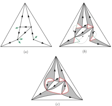
outer face admits a 3-orientation with buds iff G is simple. Moreover each outer-triangular plane G graph has a unique 3-orientation with buds satisfying the following properties (see Figure 1.a):
• Outer-accessibility: from any vertex, there is an oriented path toward the outer boundary.
• Minimality: there is no clockwise circuit.
• Local property at buds: the next half-edge after each bud in clockwise order around the incident vertex is either a bud or an outgoing edge. In particular, if a vertex carries two buds, they must be adjacent. This orientation is called the canonical 3-orientation
with buds of G.
In an outer-triangular plane graph endowed with its canonical 3-orientation with buds, an inner vertex with
i (0≤ i ≤ 2) buds is called a vertex of type i.
2.2 Canonical orientations for eulerian triangu-lations. A 1-orientation of an eulerian triangulation is
a partial orientation without buds such that outer edges are unoriented, each outer vertex has outdegree 0, each inner vertex has outdegree 1, and each inner dark tri-angle has one edge oriented counterclockwise while the other two are unoriented. The following holds:
1In a similar spirit, a recent bijection due to Ambjørn and
Budd [2] makes it possible to simplify the shape of the tree containing the information on the distance-profile of a map, using quadrangulations as intermediate structures.
(a) (b)
(c)
Figure 3: (a) An outer-triangular plane graph endowed with its canonical 3-orientation with buds, (b) after inflation and (c) after merging, the resulting eulerian triangulation endowed with its canonical 1-orientation.
Theorem 2.2. ([7, 5]) Each eulerian triangulation
has a unique 1-orientation with no circuit (this is easily seen to be equivalent to an outer-accessibility property, i.e., the existence of an oriented path to the outer bound-ary from each inner vertex). We call it the canonical
1-orientation.
In an eulerian triangulation endowed with its canonical 1-orientation, we call base-edge (drawn in red on figures) of a dark inner triangle f the edge following the unique oriented edge of f in clockwise order around f . A light triangle with i ∈ {0, 1, 2, 3} incident non-base edges is called a light triangle of type i.
2.3 Bijection between outer-triangular plane graphs and eulerian triangulations. We use the
canonical orientations to derive the main bijective result of this article:
Theorem 2.3. There is a bijection between
outer-triangular plane graphs and eulerian triangulations. Each inner edge of the plane graph corresponds to an in-ner dark triangle. Each inin-ner vertex of type i∈ {0, 1, 2} of the plane graph corresponds to a light triangle of type i, and each inner face corresponds to a light tri-angle of type 3.
Proof. Let C be an outer-triangular plane graph
en-dowed with its canonical 3-orientation with buds. Inner edges and inner vertices will be inflated in the following way:
• Each inner edge becomes a dark triangle whose
basis is the origin of the edge,
• each inner vertex becomes a light triangle whose
edges come from its former outgoing half-edges (including buds).
↔
↔ ↔
↔
After inflation, former inner faces of degree d+3 (d≥ 0) have now degree 2d + 3 (the d incident buds have turned into edges). Considering edges coming from buds as opening parenthesis, and remaining edges as closing parenthesis, one can form a clockwise parenthesis sys-tem leaving 3 edges unmatched, see Figure 4. Hence, af-ter merging the matched edges, the 3 unmatched edges form a light triangle. This ensures that each face is a triangle in the resulting map. Moreover, the edges cre-ated by the inflation are incident to a dark and a light faces, except for edges coming from buds, which are in-cident to two light faces. After merging, these edges are necessarily incident to a dark face as well. Therefore the triangulation is properly bicolored and is an eulerian tri-angulation (the outer face, which is left unchanged, is colored dark).
↔
Figure 4: Generic situation in a face of degree 4 + 3.
The resulting eulerian triangulation itself is en-dowed with an orientation (without buds). After infla-tion, each inner dark triangle carries one counterclock-wise oriented edge, and the vertex at the right extremity
of the base-edge has outdegree 1. Other vertices (com-ing from buds) have no outgo(com-ing edge before merg(com-ing. The merging ensures that these vertices are merged with vertices of outdegree 1, without creating any circuit, and preserving oriented paths from inner vertices to the outer boundary. Therefore we obtain the canonical 1-orientation for eulerian triangulations.
Conversely, starting from an eulerian triangulation endowed with its canonical 1-orientation, each transfor-mation can be easily reversed. Edges that have been merged are exactly the non-base edges in light triangles of type 1 or 2. Let a dark peak incident to a vertex be the two consecutive edges of a single dark triangle incident to this vertex. Note that, in clockwise order around a vertex, a dark peak can be either black-black, red-black or black-red. Moreover, there is exactly one red-black peak around a vertex since each vertex has outdegree 1.
In a first step, at each light triangle of type 1 or 2, untie a black-red dark peak as in Figure 5 (these operations have to be thought as done simultaneously at each light triangle of type 1 or 2):
→
→
→
→
(a)
(b)
Figure 5: Separation in (a) a light triangle of type 1, and (b) a light triangle of type 2.
In the resulting untied map, light triangles of type 3 have become light faces of degree 2d + 3 (for some
d ≥ 0), while other triangles are left unchanged. It
is easy to check that the light triangles of type 0, 1 or 2 are vertex-disjoint (this follows from the fact that, in a 1-orientation, around any inner vertex v, there is just one corner incident to v in a light face such that the clockwise-most edge of the corner is a base-edge). Hence light triangles of type 0, 1 or 2 can be contracted independently into vertices of the same type, and inner dark triangles into oriented edges, which yields an outer-triangular plane graph endowed with a 3-orientation with buds.
Untied edges were all unoriented, thus accessibility is preserved in the untied map for any vertex but for
those duplicated in the separation process. When dark triangles are contracted, those vertice are merged with the ones having an outgoing edge, which guarantees outer-accessibility. The local property at buds is also readily checked to be satisfied (see Figure 5). It remains to show that the orientation is minimal. Suppose it is not. Then by outer-accessibility, it must have a clockwise cycle C that such that any edge incident to
C from the inside of C is directed out of C. Clearly
such a cycle C had to be already present in the untied map (C has not been affected by the contraction step), and also before the separation process, a contradiction. Therefore the output is an outer-triangular plane graph endowed with its canonical 3-orientation with buds.
2.4 Bijection with oriented binary trees. In this
subsection, we follow the reformulation given in [5] of the bijection for eulerian triangulations due to Bousquet-M´elou and Schaeffer [7] (their construction applies actually to more general objects called constel-lations). We then make some simplifications.
Starting from an eulerian triangulation T , where vertices are drawn as circles, one obtains a binary tree as follows:
• Endow T with its canonical 1-orientation.
• Put a dark square vertex in each inner dark
trian-gle, and a light square vertex in each light triangle.
• Apply the local rule indicated in Figure 6 to each
edge of T .
• Remove every edge of T , and the 3 outer vertices.
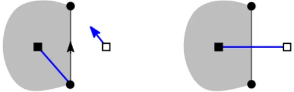
Figure 6: Local rule of the bijection between eulerian triangulations and binary trees.
Claim 2.1. ([7, 5]) The above construction is a
bijec-tion between eulerian triangulabijec-tions and unrooted binary trees with
• two types of leaves: round leaves and (extremities of ) buds,
• two types of inner nodes: dark squares (adjacent to one round leaf and two light squares) and light
(a) (b)
(c) (d)
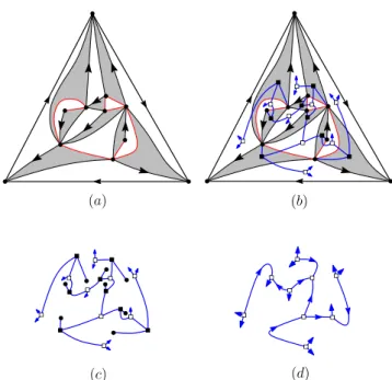
Figure 7: (a) An eulerian triangulation endowed with its canonical 1-orientation, (b) applying the local rule, (c) the resulting bicolored binary tree and (d) the simplified oriented binary tree.
• and such that each dark square is adjacent to two light squares and one round leaf.
Each inner dark triangle corresponds to a dark square of the binary tree, and each light triangle to a light square. Each inner edge corresponds to an edge (excluding buds) of the binary tree, and each inner vertex to a round leaf.
This kind of binary tree can be further simplified thanks to the particular neighborhood of each dark square: one can replace each dark square and its adjacent round leaf by an oriented edge as represented in Figure 8. After simplification, one obtains a binary tree with only light square inner nodes and whose leaves are the former buds, hence an oriented binary tree. The full process is illustrated in Figure 7. This gives the following result, which together with Theorem 2.3 implies Theorem 1.1.
Theorem 2.4. ([7] reformulated in [5]) There is
a bijection between eulerian triangulations and oriented binary trees. Each inner dark triangle corresponds to an inner edge of the binary tree. Each light triangle of type
0≤ i ≤ 3 corresponds to an inner node of outdegree i.
3 Counting results
3.1 Exact counting. Let C be an outer-triangular
plane graph, E the corresponding eulerian triangulation
↔
Figure 8: Simplification of the binary trees.
and T the corresponding oriented binary tree. Looking at the local rules (see Figures 6 and 8), one sees that each inner dark face of E yields an oriented inner edge and a leaf in T —these are considered as matched — and each of the 3 outer edges of E yields a leaf (no inner edge) in T . These 3 special leaves of T are called
exposed, the other ones (non-exposed) being matched
with the inner edges of T . The 3 exposed leaves naturally correspond to each of the 3 outer edges of
E, which are also the 3 outer edges of C. Hence, by
Theorem 1.1, rooted outer-triangular plane graphs with
n edges and i inner faces (n− i − 2 inner vertices) are in
bijection with oriented binary trees rooted at an exposed leaf, with n leaves and i sources (n− i − 2 non-source inner nodes).
LetU be the family of oriented binary trees rooted at a leaf, and letV be the family of oriented binary trees rooted at a leaf, with the edge incident to the root-leaf reversed (thus the inner node adjacent to the leaf is never a source, moreover the root-leaf is not considered as a source). Let U ≡ U(x, z) (resp. V ≡ V (x, z)) be the generating function of U (resp. V) where x marks the number of non-source inner nodes and z marks the number of non-root leaves. By a classical decomposition at the root (into a left subtree and a right subtree), U and V are given by
(3.3) {
U = (z + V )2+ 2xU (z + V ) + xU2, V = x(z + U + V )2.
Note that, for x = 1, by symmetry we have U =
V and thus U = (z + 2U )2, which gives U =
∑ n≥1 2n−1 n+1 (2n n ) zn+1.
Proposition 3.1. Let C be the family of rooted
outer-triangular plane graphs, and let C ≡ C(x, z) be the generating function of C where x marks the number of inner vertices (all vertices except the 3 outer ones) and z marks the number of edges. Then we have the two following expressions:
(3.4) ∂C
∂z = 3U, C = zU − UV, where U and V are given by (3.3).
Proof. The first expression is just a consequence of the
M
M
M
C
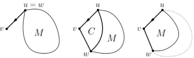
u = w u u v v v w wFigure 9: Decomposition of a plane graph along the root: 3 cases.
tree, 3 are exposed, so that C = 3∫ U dz. The second
expression follows from the property that, in an oriented binary tree, the non-exposed leaves are matched with the inner edges, and from the fact that U V is clearly the generating function of oriented binary trees with a marked inner edge. Thus, since zU is the generating function of oriented binary trees rooted at a leaf, we conclude that zU − UV is the generating function of oriented binary trees rooted at an exposed leaf.
LetM be the family of rooted plane graphs (with at least one edge), and let M ≡ M(x, z) be the generating function of M, where x marks the number of vertices and z marks the number of edges. We can now easily express M (x, z) from C(x, z). Consider a rooted plane graph γ, call u the origin of the root-edge, v the end of the root-edge, and w the next vertex after v in counterclockwise order around the root-face. Three cases can happen, as shown in Figure 9:
1. u = w, i.e., the root edge is a pending leg (with v of degree 1), and there is a rooted plane graph γ′ (possibly reduced to a vertex) hanging at u; 2. u and w are not equal but are adjacent in γ, then
γ naturally decomposes (cutting along the edge {u, w}) into a map in C and a map in M;
3. u and w are not equal nor adjacent, in which case γ is uniquely obtained from some γ′ ∈ C by deleting the outer edge that follows the root-edge in a clockwise walk around the outer face.
This yields
(3.5) M = xz(x + M ) + xz
−1CM + x3z−1C
⇒ M = x2z(1+xC/z2)
1−xz(1+C/z2),
and by Proposition 3.1 we obtain:
Proposition 3.2. The generating function M ≡
M (x, z) of rooted plane graphs by the number of ver-tices and the number of edges is expressed as
(3.6) M = x
2z + x3U· (1 − V/z)
1− xz − xU · (1 − V/z),
where U and V are given by (3.3).
3.2 Asymptotic counting. This section gives asymptotic estimates for the number of rooted plane graphs (and labeled connected graphs embedded on the sphere), which follow rather directly from the ex-pressions in Section 3.1 and the application of suitable lemmas from singularity analysis (taken from [12], the terminology used here is taken from [9, Sec. 2]). For a bivariate series f (x, z), for each x > 0, let ρ(x) be the radius of convergence of z→ f(x, z). Then ρ(x) is called the singularity function of f (x, z) with respect to z. A point (x0, z0) such that z0 = ρ(x0) is called
a singular point of f (x, z). Let (x0, z0) be a singular
point of f (x, z) such that ρ′(x0) ̸= 0 and ρ(x) is
analytically continuable to a complex neighborhood of
x0. Then, for α a positive half-integer, f (x, z) is said to
admit a singular expansion of order α around (x0, z0)
with leading variable z, if there exist functions g(x, z) and h(x, z) analytic around (x0, z0), with h(x0, z0)̸= 0,
such that, in a complex neighborhood of (x0, z0),
f (x, z) = g(x, z) + h(x, z)· (1 − z/ρ(x))α.
The singular expansion is called strong if f (x, z) is analytically continuable to a complex domain of the form Ω = {(x, z) | |x| ≤ x0+ δ, |z| ≤ z0+ δ}\{1 −
z/ρ(x) ∈ R≤0} for some δ > 0. It can be shown
(see [12]) that then f (x, z) also has a strong singular expansion at (x0, z0) with leading variable x, hence it is
not necessary to mention which variable is taken as the leading variable.
A first task for us is to determine the singular points of U (x, z). It is easy to see that the singular points are the same for U (x, z) as for V (x, z). We have
U = x(z + U + V )2+ (1− x)(z + V )2 = V + (1−
x)(z + V )2, so that V = x(z + 2V + (1− x)(z + V )2)2,
so we have an explicit polynomial equation of the form
H(x, z, V ) = 0, satisfied by V ≡ V (x, z). Hence we
classically have to look for solutions in {x, z} of the system{H(x, z, V ),∂H∂V(x, z, V ) = 0}. With the help of a computer algebra system (to take the resultant of the two equations according to V ), we find and check that the singular points cover the curve parametrized by
(3.7)
{
x = (u+1)(uu3(u−2)−1)3
z = (2 u+1)(u4(u+1)(u−2)u−1)3 over u∈ (0, 1).
Lemma 3.1. The generating functions U (x, z) and
V (x, z) have a strong singular expansion of order
1/2 around any of their singular points, which are
parametrized by (3.7).
Proof. There are general conditions, given in [11],
un-der which a bivariate (more generally a multivariate) generating function f (x, z) that appears in a positive
equation-system has a strong singular expansion of or-der 1/2 at any singular point (z0, u0). These conditions
(irreducibility, aperiodicity,...) are readily checked to be satisfied by (3.3).
We will use the following lemma from [12] (see also [9, Sec.2]):
Lemma 3.2. Let f (x, z) be a bivariate generating
func-tion that admits a strong singular expansion of order α at a singular point (x0, z0). Then the generating
func-tion ∫ f (x, z)dz admits a strong singular expansion of order α + 1 at (x0, z0).
Lemma 3.3. The generating functions C(x, z) and
M (x, z) have the same singular points as U (x, z). In addition, at any singular point (x0, z0), C(x, z) and
M (x, z) admit a strong singular expansion of order 3/2.
Proof. For C(x, z) it is a direct consequence of C =
∫
U dz and of Lemmas 3.1 and 3.2. We now con-sider M (x, z). We have (where the symbol ⪯ means “coefficient-wise smaller”):
x3C(x, z)⪯ M(x, z) ⪯ x3C(x, z)/z2,
the lower bound is due toC being a subfamily of M, and the upper bound is due to the fact that, for an object in M, the operation of adding a vertex of degree 2 in the outer face connected to the two extremities of the root-edge yields an object in C. These bounds and the fact that M (x, z) has a specific rational expression (3.5) in terms of C(x, z), x and z easily imply that M (x, z) “inherits” from C(x, z) the property of having a strong singular expansion of order 3/2 at (x0, z0).
We now turn our attention to embeddings on the sphere. Let gi,n be the number of connected graphs
embedded on the sphere with n edges and i vertices, the vertices having distinct labels in [1..i]. And let
G(x, z) = ∑i,ni!1gi,nxizn be the corresponding
(expo-nential) generating function. Let mi,nbe the number of
rooted plane graphs with i vertices and n edges. There are i! distinct ways to label the vertices of a rooted plane graph with i vertices; and there are 2n ways to root a connected labeled graph embedded on the sphere (one takes the face on the right of the root-edge as the outer face). Since these are two ways to construct the same objects (rooted labeled) we have i! mi,n= 2n gi,n, hence
(3.8) 2z∂G
∂z(x, z) = M (x, z).
Hence, by Lemmas 3.2 and 3.3 we obtain:
Lemma 3.4. The generating function G(x, z) has the
same singular points as U (x, z). In addition, at any singular point (x0, z0), G(x, z) admits a strong singular
expansion of order 5/2.
From this we can obtain asymptotic estimates for the coefficients of G(x, z) (as well as C(x, z) and
M (x, z)) using the following transfer lemma [14]:
Lemma 3.5. Let f (x, z) be a generating function that
admits a strong singular expansion of order α at any singular point, and let ρ(z) be the singularity function of f (x, z) with respect to x. Then for any z0 > 0 (in
particular z0 = 1) the coefficient fn(z0) = [xn]f (x, z0)
satisfies
fn(z0)∼ c n−α−1γn.
where γ = 1/ρ(z0) and c is some (analytically
com-putable) positive constant.
Assume that µ(z) := −zρ′(z)/ρ(z) is strictly
increasing, and define a = limz→0µ(z) and b =
limz→+∞µ(z). For any fixed µ ∈ (a, b) let z0 be
the positive value where µ(z0) = µ and let γ(µ) =
1/ρ(z0). Then there is a positive (analytically
com-putable) constant c(µ) such that the coefficients fn,m:=
[xnzm]f (x, z) satisfy
fn,⌊µn⌋∼ c(µ)n−α−3/2γ(µ)n when n→ ∞.
In our case (singularity function of U (x, z)), we easily check (with a computer algebra system) that a = 1 and b = 3. Together with Lemma 3.4, the second part of Lemma 3.5 yields Theorem 1.2; while the first part ensures for instance that the number cn of connected
graphs embedded on the sphere and having n (labeled) vertices satisfies asymptotically cn ∼ n! c n−7/2γn,
where c and γ are computable, γ ≈ 34.2672. This is to be compared with the asymptotic number ˜cn of
connected planar graphs with n vertices given in [16], which is asymptotically ˜cn ∼ n! ˜c n−7/2γ˜n, with ˜γ ≈
27.2269. Hence, the expected number of embeddings on the sphere of a random planar graph with n (labeled) vertices is asymptotically a· bn, with b≈ 1.2586.
4 Application to random generation of plane graphs
4.1 Sampling rooted plane graphs by edges. We
first give an easy uniform random sampler for the family
Mm of rooted plane graphs with m edges.
Let Cm be the set of rooted outer-triangular plane
graphs with m edges. As explained in Section 3.1, the bijection of Theorem 1.1 can be formulated as an m-to-3 correspondence between Cm and the familyUm of
rooted oriented binary trees with m leaves. Uniform sampling in Um can classically be done in linear time
(generate a rooted binary tree and flip a coin at each inner edge to choose the orientation). Hence, composing with the bijection of Theorem 1.1 (seen as an m-to-3 correspondence) yields a linear-time uniform random sampler forCm.
Now, let eCm ⊂ Cm be the set of rooted
outer-triangular plane graphs with m edges such that the outer vertex opposite to the root-edge has degree 2. For
C ∈ eCm+2, let ϕ(C)∈ Mm be the rooted plane graph
obtained from C by deleting the outer vertex opposite to the root-edge (and its two incident edges). Clearly, ϕ is a bijection between eCm+2 and Mm. Hence a uniform
random sampler for Mm is obtained by repeatedly
calling the sampler forCm+2until the generated object
C is in eCm+2, and then returning ϕ(C).
Proposition 4.1. The above procedure yields a
uni-form random sampler for rooted plane graphs with m edges in expected time O(m).
Proof. At each trial the probability of success (of being
in eCm+2) is | eCm+2|/|Cm+2| = |Mm|/|Cm+2|. The
expressions of C(z) and M (z) yield (using transfer lemmas) asymptotic estimates of the form c 8mm−5/2
for both |Cm+2| and |Mm|. Thus, the probability of
success tends to a positive constant as m → ∞ (hence is bounded from below uniformly in m). Moreover, by an elementary probability identity, the expected complexity of the sampler for Mmequals the expected
complexity of the sampler for Cm+2 (which is O(m))
divided by the probability of success.
4.2 Sampling rooted plane graphs by vertices and edges. We now explain how to generate rooted
plane graphs by vertices and edges. Our generator relies on the methodology of Boltzmann sampling [13]. This is similar to the sampler developed for planar graphs in [15], but the sampler described here is much simpler and one can sample exactly at the singularity. We denote U = ∪mUm, C =
∪
mCm, and eC =
∪
mCem. A
Boltzmann sampler ΓU (x, z) for the classU of oriented
binary trees is an algorithm which outputs each T ∈ U with probability proportional to xnzm, where n is the
number of non-source inner nodes and m is the number of leaves. As explained in [13], a grammar specification such as (3.3) can be automatically translated into a Boltzmann sampler ΓU (x, z), such that the complexity of generating a tree T ∈ U is linear in m. Via the m-to-3 correspondence between Um and Cm, ΓU (x, z) yields a
random generator ΓC(x, z) where each C∈ C is drawn with probability proportional to mxnzm, where n is the number of vertices and m is the number of edges, and the cost is linear in m.
From this generator ΓC(x, z) we can easily obtain random samplers for rooted plane graphs, either in the form of an exact-size or an approximate-size random sampler (in the first case, the “target-domain” for the pair (#vertices, #edges) is a singleton (n, m), in the second case, the target-domain is of the form [n(1−
ϵ), n(1 + ϵ)]× [m(1 − ϵ), m(1 + ϵ)]). As explained in [13],
by appropriately tuning x and z in ΓC(x, z), and using early-abort technique, one can obtain efficient exact-and approximate-size samplers. Indeed, let µ := m/n and let z0be the value of z associated to µ as explained
in the second part of Lemma 3.5, and let x0 be the
value such that (x0, z0) is a singular point of U (x, z).
We consider the random sampler that consists in calling ΓC(x0, z0) until the generated plane graph G = (V, E)
is in eC and the pair (n, m) given by n := |V | − 1, m :=
|E|−2 is in the target-domain (each call to ΓC(x0, z0) is
aborted as soon as these numbers are already too large), and then returning G′= ϕ(G), which has n vertices and
m edges.
Proposition 4.2. When m/n is bounded away from 1 and 3 (by a fixed positive constant c > 0), the
expected cost of the random sampler for rooted plane graphs is O(n5/2) in exact-size sampling and is O(n/ϵ)
in approximate-size sampling. (The constant in the big O depends on c.)
As in [15] it is also possible to get an exact-size (target-domain n) and approximate-size (target-domain [n(1− ϵ), n(1 + ϵ)]) random sampler according to the number of vertices, with no target domain for the number of edges. The technique is similar except that one has to call the Boltzmann sampler ΓC(x0, 1)
—with x0the value such that (x0, 1) is singular— until
the rooted plane graph obtained is in eC and the number of vertices is in the target-domain (again each call to ΓC(x0, 1) is aborted as soon as the number of vertices
is too large). In this case, the expected cost is O(n2) for
exact-size sampling and O(n/ϵ) for approximate-size sampling.
Acknowledgments. We are very grateful to Marc Noy for
letting us know about the simplified expression (1.1), which was the starting point of this work. We also thank Valery Liskovets and Sergei Chmutov for an interesting email correspondence on related questions, and Dominique Poulalhon for an interesting discussion on orientations for planar constellations.
References
[1] M. Albenque and D. Poulalhon. Generic method for bijections between blossoming trees and planar maps. arXiv:1305.1312, 2013.
[2] J. Ambjørn and T.G. Budd. Trees and spatial topology change in causal dynamical triangulations. J. Phys. A: Math. Theor., 46(31):315201, 2013.
[3] C. Banderier, P. Flajolet, G. Schaeffer, and M. Soria. Random maps, coalescing saddles, singularity analysis, and Airy phenomena. Random Structures Algorithms, 19(3/4):194–246, 2001.
[4] O. Bernardi and ´E. Fusy. Unified bijections for maps with prescribed degrees and girth. J. Combin. Theory Ser. A, 119(6):1352–1387, 2012.
[5] O. Bernardi and ´E. Fusy. A master bijection for planar hypermaps with general girth constraints. In preparation, 2013.
[6] M. Bona. Exact enumeration of 1342-avoiding permu-tations; a close link with labeled trees and planar maps. J. Combin. Theory Ser. A, 80:257–272, 1997.
[7] M. Bousquet-M´elou and G. Schaeffer. Enumeration of planar constellations. Adv. in Appl. Math., 24(337-368), 2000.
[8] J. Bouttier, P. Di Francesco, and E. Guitter. Planar maps as labeled mobiles. Electron. J. Combin., 11(1), 2004.
[9] G. Chapuy, ´E. Fusy, O. Gim´enez, B. Mohar, and M. Noy. Asymptotic enumeration and limit laws for graphs of fixed genus. J. Combin. Theory Ser. A, 118(3):748–777, 2011.
[10] R. Cori and B. Vauquelin. Planar maps are well labeled trees. Canad. J. Math., 33(5):1023–1042, 1981. [11] M. Drmota. Systems of functional equations. Random
Structures Algorithms, 10(1-2):103–124, 1997.
[12] M. Drmota, O. Gim´enez, and M. Noy. Vertices of given degree in series-parallel graphs. Random Structures Algorithms, 36(3):273–314, 2010.
[13] P. Duchon, P. Flajolet, G. Louchard, and G. Schaeffer. Boltzmann samplers for the random generation of combinatorial structures. Combin. Probab. Comput., 13(4–5):577–625, 2004. Special issue on Analysis of Algorithms.
[14] P. Flajolet and R. Sedgewick. Analytic combinatorics. Cambridge University Press, 2009.
[15] ´E. Fusy. Uniform random sampling of planar graphs in linear time. Random Struct. Algorithms, 35(4):464– 522, 2009.
[16] O. Gim´enez and M. Noy. Asymptotic enumeration and limit laws of planar graphs. J. Amer. Math. Soc., 22:309–329, 2009.
[17] M. Noy. Private communication, Sept. 2012.
[18] G. Schaeffer. Conjugaison d’arbres et cartes combina-toires al´eatoires. PhD thesis, Universit´e Bordeaux I, 1998.
[19] G. Schaeffer. Random sampling of large planar maps and convex polyhedra. In Proceedings of the ACM
Symposium on Theory of Computing, pages 760–769. ACM, New York, 1999.
[20] W. T. Tutte. A census of planar maps. Canad. J. Math., 15:249–271, 1963.