Designing a congestion control plane datapath with QUIC

Designing a Congestion Control Plane Datapath with

QUIC

by

Deepti Raghavan

Submitted to the Department of Electrical Engineering and Computer

Science

in Partial Fulfillment of the Requirements for the degree of

Master of Engineering in Electrical Engineering and Computer Science

at the

MASSACHUSETTS INSTITUTE OF TECHNOLOGY

September 2018

© 2018 Deepti Raghavan. All rights reserved.

The author hereby grants to M.I.T. permission to reproduce and to

distribute publicly paper and electronic copies of this thesis document in

whole or in part in any medium now known or hereafter created.

Author . . . .

Department of Electrical Engineering and Computer Science

June 27, 2018

Certified by . . . .

Hari Balakrishnan

Fujitsu Professor

Thesis Supervisor

Accepted by . . . .

Katrina LaCurts

Chair, Master of Engineering Thesis Committee

Designing a Congestion Control Plane Datapath with QUIC

by

Deepti Raghavan

Submitted to the Department of Electrical Engineering and Computer Science on June 27, 2018, in partial fulfillment of the

requirements for the degree of

Master of Engineering in Electrical Engineering and Computer Science

Abstract

This work explores developing datapaths for the recently proposed Congestion Control Plane(CCP) architecture and uses QUIC as a case study to build and evaluate an example datapath. The CCP moves congestion control logic off of the datapath into a separate agent running in user-space. Now, algorithm developers can write their algorithm using this API and automatically run their algorithm on any CCP enabled datapath, such as QUIC or the Linux kernel. We discuss the necessary features for datapaths to support the user-space CCP agent and develop a library, libccp, for software datapaths. We use QUIC as a case study to design a CCP datapath and evaluate various congestion control algorithms running on top of QUIC.

The evaluation focuses on four aspects: (1) Do algorithms written on CCP have the same performance as QUIC algorithms? (2) Do CCP congestion control algorithms behave similarly to their native QUIC counterparts, when run on top of QUIC? (3) How expres-sive is the CCP API? (4) Does the same algorithm, written through CCP, behave similarly across multiple datapaths? This work reveals that while CCP QUIC algorithms have sim-ilar performance for a single flow, their behavior does not exactly match the native QUIC implementations of the same algorithms without modifications. We show that CCP can provide “write once, run anywhere” semantics for congestion control, as multiple algo-rithms run across QUIC and the Linux kernel exhibit similar behavior. Finally, we evaluate the expressiveness of the CCP API by implementing two algorithms: Hybrid Slow Start and Remy.

Thesis Supervisor: Hari Balakrishnan Title: Fujitsu Professor

Acknowledgments

First and foremost, I would like to thank my advisor, Professor Hari Balakrishnan. Through the course of my undergraduate and Meng research, his guidance, enthusiasm for systems research and advice to me have been invaluable.

I have been very lucky to collaborate with a many great people through my UROP and Meng in the NMS group. I am grateful to have worked with Keith Winstein - his perspective on research has taught me a lot. To Frank Cangialosi and Akshay Narayan: it has been very rewarding to work on the CCP this past year with you. Many thanks to Prateesh Goyal, Anirudh Sivaraman, Srinivas Narayana, Venkat Arun and Mohammad Alizadeh for various helpful discussions and feedback.

Thank you to the entire NMS, group, including Vibhaa Sivaraman, Vikram Nathan, Amy Ousterhout, Ravi Netravali and Sheila Marian, for making the past couple years so enjoyable. Not only have I learned about networking, but I have slightly improved at ping pong! A special shoutout goes to Ravi for finding my coffee cup.

To my friends, Kiran Wattamwar, Nikita Kodali, and Kimberli Zhong: it really is un-clear what I would do without you. To my roommates - Shirin Shivaei, Suma Anand, and Erin Hong - thank you for all the laughter, emotional support, and ice cream trips.

Finally, I would not be where I am today without my family, who have believed in me, supported me through all my endeavours and have listened to me complain since 1995! Keshav - I have to admit you are my role model and a cool older brother. Amma and Appa: thanks for everything, you guys are the best!

Contents

1 Introduction 15

1.1 Motivation for a Congestion Control Plane . . . 16

1.2 Designing CCP Datapaths . . . 16

1.3 Contributions . . . 17

2 Related Work 19 2.1 Pluggable Congestion Control . . . 19

2.2 QUIC . . . 20

2.3 CCP . . . 21

3 Implementation: Designing CCP Datapaths 23 3.1 CCP Algorithm Interface . . . 23

3.1.1 Datapath programs . . . 24

3.2 Responsibilities of a CCP Datapath . . . 25

3.3 libccp . . . 28

3.4 Current Congestion Control Architecture in QUIC . . . 29

3.5 Integratinglibccpin QUIC . . . 31

3.5.1 Architecture . . . 31

3.5.2 Congestion Signal Measurement . . . 32

3.6 Summary of Implementation . . . 34

4 Evaluation of QUIC Datapath 35 4.1 Experimental Setup . . . 36

4.2 Toy Server Performance Limitations . . . 37

4.2.1 Sending Rate Limits . . . 37

4.2.2 Scalability . . . 38

4.3 Single Flow Behavior . . . 39

4.3.1 TCP Reno and TCP Cubic . . . 40

4.3.2 BBR . . . 43

4.3.3 Summary . . . 44

4.4 Request Completion Times . . . 44

4.5 Multiple Flow Behavior . . . 46

4.6 Discussion . . . 47

5 Writing Algorithms in CCP 49 5.1 Hybrid Slow Start . . . 50

5.1.1 Algorithm . . . 50 5.1.2 Implementation in CCP . . . 51 5.1.3 Evaluation . . . 53 5.2 Remy . . . 53 5.2.1 Background . . . 54 5.2.2 Implementation in CCP . . . 55 5.2.3 Preliminary Evaluation . . . 58

5.3 Write once, run anywhere . . . 59

List of Figures

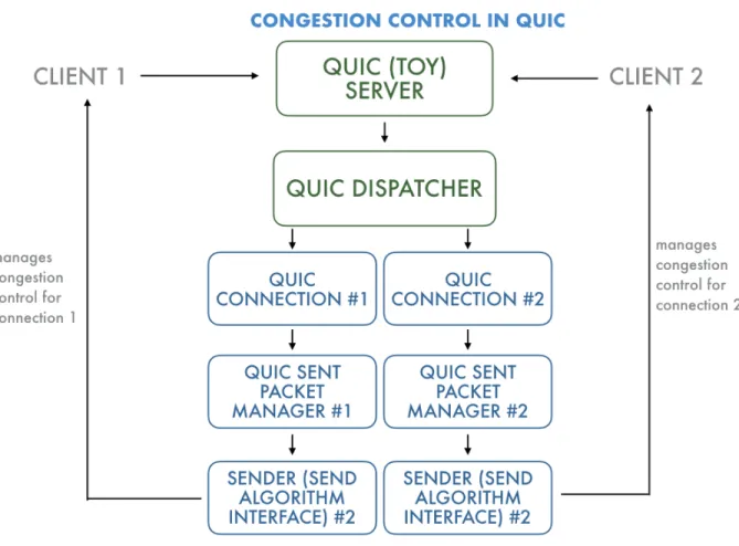
3-1 CCP BBR datapath program that implements BBR’s probe bandwidth phase. 27 3-2 Flow of congestion control within QUIC. When the toy server sees a client

request, theSimpleDispatcherobject spawns a newQuicConnectionobject that handles the connection. To manage sending packets, theQuicConnection

object creates aQuicSentPacketManager. TheQuicSentPacketManager

cre-ates aSenderobject that uses the function callbacks from theSendAlgorithmInterface

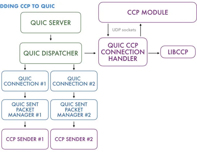
specified as the current congestion control setting. . . 30 3-3 Overview of how CCP andlibccpfit into QUIC, with the newCCPConnectionHandler

class. By having access to the relevantQuicConnection object in a call to

Set_Cwnd(), theCCPConnectionHandlerpropagates the instruction down to the correctCCPSenderobject. . . 32 4-1 Behavior of single flow setting a constant window or pacing rate at a low

and high bandwidth. At higher bandwidths, the QUIC cannot sustain the sending rate perfectly and the delays vary more. . . 37 4-2 Aggregate throughput of an increasing number of flows on a localhost

connection. The server runs Reno or Cubic, with and without CCP, and transfers a file of size 100MB to an increasing number of clients. Aggre-gate throughput is calculated as the total number of bytes transferred to all clients, divided by the maximum file transfer time of any client, averaged across 5 trials. Note that for both CCP and QUIC, aggregate throughput decreases as the number of flows increase. CCP does seem to have slightly lower throughput. . . 38

4-3 Congestion window dynamics of a single TCP Reno flow in various emu-lated environments. For most cases, the CCP Implementation of TCP Reno

seems to follow the congestion window of QUIC Reno quite closely. . . 41

4-4 Congestion window dynamics of a single TCP Cubic flow in various em-ulated environments. For most cases, the CCP Implementation of TCP Cubic seems to follow the congestion window of QUIC Cubic quite closely. 42 4-5 Downlink throughput and queueing delay for TCP Cubic and Reno over a fixed bandwidth link. The left side shows CCP, while the right side shows QUIC. . . 43

4-6 Downlink throughput and queueing delay for BBR and QUIC BBR flow. . . 43

4-7 Request completion times for a 100 MB file across Cubic, Reno and BBR for fixed (48 Mbps, 20 ms RTT), lossy (48 Mbps, 20 Ms RTT, .01% de-terministic drops) and cellular (Verizon uplink trace, 20 ms RTT) environ-ments. Cubic and Reno match almost perfectly for lossy and cellular envi-ronments and are slightly slower in the fixed link environment. The CCP version of BBR is slightly slower; this may be attributed to the different startup behavior shown in Figure 4-6. . . 46

4-8 2 CCP Cubic flows: 20.69 and 20.56 Mbps . . . 47

4-9 2 QUIC Cubic Flows: 21.94 and 21.92 Mbps . . . 47

4-10 3 CCP Cubic Flows: 14.88 Mbps, 11.94 Mbps, 11.513 Mbps . . . 47

4-11 3 QUIC Cubic Flows: 16.81 Mbps, 16.69 Mbps, 16.72 Mbps . . . 47

4-12 Throughput and queueing delay of multiple Cubic flows on a fixed link with 48 mbps bandwidth and 10 ms propagation delay. . . 47

5-1 Excerpt of Hybrid Slow Start implemented with new congestion signals that expose which sequence number is last acked, as well as which se-quence number was last sent. We omit the program variable definitions and only show the conditions to leave slow start. . . 51

5-2 Excerpt of Hybrid Slow Start implemented where packet rounds end on each minimum RTT. . . 52

5-3 Congestion window dynamics of a single TCP CCP Cubic flow with vari-ous forms of slow start, compared against QUIC CCP. With either hybrid slow start, CCP exits slow start at approximately the same time as QUIC

Cubic. . . 54

5-4 Congestion window dynamics of a single TCP CCP Reno flow with various forms of slow start, compared against QUIC CCP. With either hybrid slow start, the window evolution between CCP Reno and QUIC reno is very similar. . . 54

5-5 Fold functions that define the four congestion signals needed by Remy. The full datapath program is omitted for brevity. Here, the intersend and interreceive times via dividing the rate by a scaling factor, that converts the rate from datapath units (bytes per second) to Remy signal units (packets per millisecond). The fast ewma for the intersend and receive times are calculated with alpha as 1/8, and the slow receive ewma is calculate with alpha as 1/256. . . 57

5-6 TCP Cubic, 48 Mbps link with 20 ms RTT and 2 BDP of buffering . . . 59

5-7 TCP Reno, 48 Mbps link with 20 ms RTT and 2 BDP of buffering . . . 60

5-8 Copa, 12 Mbps link with 20 ms RTT and 2 BDP of buffering . . . 60

List of Tables

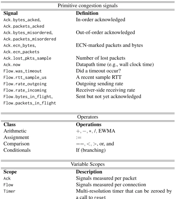
3.1 Datapath program domain specific language: primitive signals, operators, and scopes. As per the CCP API, datapaths must expose these signals and implement these operators. . . 26 3.2 Calculations used by theCCPSenderto update the primitive congestion signals. 33 4.1 Throughput and delay achieved in various fixed, cellular, and lossy

scenar-ios for CCP QUIC and QUIC Reno, Cubic and BBR flows. The lossy shells add .01% deterministic drops. The capacity of the Verizon trace varies over time, but is 4.5 Mbps on average. . . 45 5.1 Achieved localhost throughput for 2 versions of Remy: over UDP and over

Chapter 1

Introduction

Congestion control algorithms decide when endpoints should send each segment of data and has been active area of development since the the 1980s. Research has flourished recently due to new applications and network technologies. This research both includes new algorithms, such as Remy [26], Copa [4], as well as new datapaths, a term referring to any module that allows applications to interface with the network; i.e., send and receive packets.

Currently, congestion control is tightly integrated into the datapath, since a natural place to make decisions about how fast to send data is in the datapath. Example datapaths include the Linux kernel, which implements various congestion control algorithms, kernel bypass methods, such as mTCP/DPDK [9, 16, 23], specialized Network Interface Cards (“Smart NICS” [22]). One recent datapath is QUIC [18], a UDP based transport, currently used in Google chrome and YouTube connections. However, we observe that congestion control algorithms do not need to be implemented directly in the datapath. In fact, implementing congestion control in an off-datapath agent, that communicates with the datapath at regular intervals, could ease congestion control development.

If algorithms were implemented through some common off datapath agent, any dat-apath that supports this agent could run the resulting algorithms. This would introduce “write once, run anywhere” behavior - where developers could write congestion control al-gorithms once, through this agent, and run them automatically on multiple datapaths. The recently proposed Congestion Control Plane (CCP) [19, 20] architecture presents a design

for an off datapath congestion control agent. This thesis explores the core responsibilities for datapaths to support various congestion control algorithms through the CCP. We design a library to help datapaths support CCP, and we build and evaluate a datapath inside QUIC as a case study.

1.1

Motivation for a Congestion Control Plane

While various new congestion control algorithms have emerged, as well as many new data-paths, new datapaths tend to lack support for various congestion control algorithms. There are many subtle nuances in ensuring the correctness of behavior and performance of a new algorithm on a single datapath. With an architecture like CCP’s, congestion control researchers can focus on the core algorithm logic without worrying about deploying the algorithm on various datapaths. CCP enables faster congestion control development; with a simple userspace API to implement a new algorithm, developers can iterate on mistakes faster. CCP allows new capabilities, such as single off datapath agent controlling conges-tion avoidance for multiple flows at the same endpoint. The Linux kernel datapath is limited in computation in that algorithms cannot perform floating point operations. While this is not a problem for the QUIC datapath, which runs in user-space, algorithms implemented on CCP can use complex calculations such as Fast Fourier Transforms [13], or neural net-works [27] and be deployed any CCP enabled datapath. Finally, CCP enables developers to automatically run the same algorithm on different datapaths with minimal effort.

1.2

Designing CCP Datapaths

Congestion control algorithms, at their core, decide when to transmit each segment of data by using measurements, or congestion signals, taken after sending previous segments of data. For congestion control to be off the datapath, the datapath must summarize infor-mation about these congestion signals - including RTT, packets lost and received, explicit congestion notification (ECN) markings, sending and receive rates, and provide it to the off datapath agent. The datapath must also expose an interface to control sending rates

-namely an interface to set the congestion window or pacing rate for the connection. We cre-ate an exact specification of datapath responsibilities - including both the set of congestion signals the datapath should expose, as well as a simple framework to execute the directives a CCP program.

1.3

Contributions

This thesis makes the following contributions:

• Distilling the requirements for datapaths to support a wide array of congestion control algorithms and designing a framework,libccp, that contains a reference implemen-tation for CCP’s datapath component.1 _{libccp is available at https://github.com/} ccp-project/libccp

• A case study of usinglibccpto design a CCP datapath inside QUIC, and an evalua-tion of the fidelity of this QUIC datapath: is the performance reasonable? Does the API give congestion control developers the same flexibility as the QUIC pluggable congestion control interface? This implementation is available at https://github. com/ccp-project/ccp-quic.

• Running various algorithms on both the Linux kernel and QUIC, to show the benefits of “write once, run anywhere” behavior.

• A discussion of the expressiveness of the CCP API.

1_{This portion of the work was done jointly with my collaborators on our CCP paper, to be published at}

Chapter 2

Related Work

2.1

Pluggable Congestion Control

Multiple frameworks include pluggable congestion control interfaces. Linux’s pluggable TCP API [8] provides various statistics for each flow, including delay, rates averaged over the past RTT, ECN information, and packet loss statistics. This API also provides a call-back for algorithms to update any state after each ACK and on timeouts, and directives to set the congestion window and pacing rate. icTCP [14] is a modified TCP stack in the Linux kernel thay allows user space progreams to modify specific TCP-related variables such as the congestion window, slow start threshold, receve window size and retransmission time-out. HotCocoa [2] introduces a domain specific language meant to compile congestion control algorithms directly into programmable hardware, to increase efficiency in packet processing. CCP, in contrast, runs in userspace, and gets the benefit of various userspace computational libraries. CCP could allow algorthms that contain various floating point operations and Fourier transforms. QUIC [18, 25] provides a similar pluggable conges-tion control interface that offers similar statistics per flow, and callbacks when there are timeouts, packets are sent, or ACKs are received.

The CCP kernel and QUIC datapaths in fact use Linux’s and QUIC’s pluggable con-gestion control interfaces for their implementations. CCP extends the functionality offered by these interfaces because it also allows for asychronous control, or control decisions not tied to the ACK clock. QUIC and the kernel allow developers to implement callbacks for

packet arrivals and timeout (and, in the case of QUIC, sending packets). CCP provides an extra layer of control, off the datapath, not tied to sending or receiving packets.

eBPF [11] allows developers to deifne programs that can be safely executed in the Linux kernel. These programs can be compiled just in time and attached to various kernel functions for debugging. TCP BPF [5], built on top of eBPF, allows endpoints to customize TCP connection settings, such as the TCP buffer size, by matching on the flow data. Whie CCP could use eBPF capabilities to gather measurements for congestion control algorithms in the Linux kernel, this would not work in other CCP enabled datapaths, such as QUIC.

2.2

QUIC

The QUIC (Quick UDP Internet Connections) transport protocol, which runs over UDP, aims to improve performance for HTTPS traffic. It aims to reduce Head-of-line blocking delay by supporting multiple streams within a single connection; when a packet is lost, it only affects the streams whose data was in this packet. Data on other streams can continue to be processed for the application without any delay. QUIC connections are also com-pletely encrypted; the protocol also replaces TCP and TLS and aims to be 0-RTT. After a successful handshake the client caches information about the server, causing subsequent connections to be established without any round trip times.

As discussed in Section 2.1, QUIC offers a pluggable congestion control interface; the default congestion control option is a variant on TCP Cubic. QUIC uses a different loss recovery mechanism than regular TCP. In TCP, a retransmission carries the same sequence number as the original transmission. When an ACK is received, it is unclear if this ACK is for the original transmission or for a retransmission. By contrast, QUIC assigns a new sequence number to every packet, including sequence numbers. The ACKs also record the delay between when the packet was received and when the acknowledgement was sent, so RTT measurements are as accurate as possible. In addition, QUIC allows up to a range of 256 ACK frames, while TCP allows only up to 3, so QUIC is more resilient to loss than TCP, with the SACK (selective acknowledgements) protocol. Adding CCP to QUIC enhances the congestion control options to QUIC; these algorithms benefit from QUIC’s

improved loss recovery.

2.3

CCP

CCP, described in [19], provides three broad benefits:

1. The ability to write algorithms once and run them on any CCP enabled datapath. This work discusses the QUIC datapath, but we have also implemented a CCP datapath in the Linux kernel and mTCP.

2. A higher pace of development for congestion control development. Instead of wor-rying about the intricacies the datapath structures and functions, a congestion control developer can focus on the core logic required for their algorithm.

3. New capabilities, including new algorithms that include complex calculations such as fourier transforms, as well as the ability to group congestion control decisions together for multiple flows at one host.

The current user level CCP implementation,Portus, is written in Rust and provides bind-ings in Python. Experiments with the Linux kernel show that CCP algorithms behave similarly to the kernel versions of those algorithms, and, on the kernel, only incur a modest CPU overhead.

Chapter 3

Implementation: Designing CCP

Datapaths

A CCP compatible datapath needs to accurately enforce the congestion control algorithm sent down by the CCP userspace module. Algorithm developers need not worry about datapath specific concerns, such as accurately measuring signals and setting the correct sending rate. Furthermore, once a datapath correctly implements support for CCP, this automatically enables support for all CCP algorithms.

In order to implement support for CCP in both QUIC and the Linux kernel, we designed a library, libccp, to make the life of the datapath developer easier. libccp clearly defines the requirements for a CCP datapath as well as handles CCP specific computation common to all datapaths. We briefly discuss the CCP user-space algorithm interface, and then we describe the implementation oflibccpand how we uselibccpto design a CCP datapath in QUIC.

3.1

CCP Algorithm Interface

In the Linux kernel, congestion control decisions are tied to the ACK clock - algorithm computation is typically invoked everytime a packet ackowledgement arrives in the net-working stack. QUIC provides an additional callback for algorithm functionality when packets are sent. This restricts algorithm computation time to the interarrival time of ACKs

or intersend time of packets; congestion control algorithms with complex computation may not perform well at high rates. CCP, in contrast, provides both in-datapath control function-ality and asynchronous control functionfunction-ality. CCP requires algorithms to be split into two separate components explicitly: a program to execute in an off-datapath CCP agent and a separate program to execute within the datapath itself. Because a portion of the conges-tion control algorithm is now run off the datapath, the datapath must summarize congesconges-tion signal information somehow and send it to the CCP agent. At user specified intervals, the datapath reports congestion signal information to the CCP agent; the CCP agent can use these measurements to perform rate control decisions asynchronously from the datapath.

The CCP API is currently written in Rust, with bindings in Python. Users must write two functions that contain algorithm functionality to be run outside of the datapath:

• onCreate - Establishes algorithm state when a flow is created. Users must install some datapath program here, or else they will not get any measurements from the datapath to perform computation.

• onReport- Callback when the datapath sends a report back to the CCP agent. This may involve some more complicated calculation that requires special user-space li-braries, such as FFTs or neural networks.

3.1.1

Datapath programs

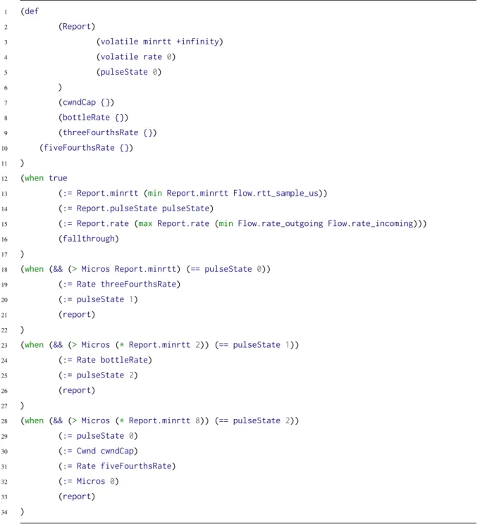
Datapath programs are written in a simple, event driven, domain specific language. These programs exist to provide an in-datapath, per-ACK execution environment for congestion control algorithms to update state variables per ACK and perform control actions, in re-sponse to conditions triggered by thes variables. Figure 3-1 shows a CCP BBR program, that implements BBR’s probe bandwidth phase. The first block of the program defines cus-tom variables for the user to measure; variables within the Report block are sent back to the CCP agent on reports. The volatile marker specifies these variables should be reset to their original values after each report. This is followed by a series of conditions, each with a set of instructions to execute if the condition evaluates to true.

The very first condition,when true, specifies that the block beneath should be executed everytime the program is done; here, datapath programs typically contain fold functions. Fold functionsare custom summaries over primitive congestion signals. Datapath programs have read access to various primitive congestion signals, exposed by the datapath and up-dated per ACK. Table 3.1 lists the set of congestion signals the CCP API specifies for datapaths to provide. The BBR program uses the RTT estimate for the flow to keep track of the minimum RTT. It also estimates the bottleneck rate of the link as the minimum of the measured receive rate and send rate.

Programs can also define conditions based on variable values and perform control ac-tions, such as updating the sending rate, or sending a report up to the CCP agent, in re-sponse. The following three blocks show the BBR sending pattern: it probes for the link rate by setting the rate to be 1.25x the current rate after 1 RTT. To drain a queue that may have been create, it then sets the rate to be 0.75x the rate after one more RTT, and then it finally sets the rate as the bottleneck rate estimate after 8 RTTs. The BBR also sends a report to the datapath after 1, 2 and 8 RTT’s have passed. Section 4.3.2 shows results for our BBR implementation in CCP.

3.2

Responsibilities of a CCP Datapath

A CCP datapath has four main responsibilities. • Establish an IPC mechanism.

• Enforce congestion windows and pacing rates.

• Update the congestions signals listed in Table 3.1 as ACKs are received.

• Parse and serialize the datapath program sent by the CCP agent, and execute the datapath program every ACK. This may cause the datapath to send a report up to the CCP agent.

First, it must communicate with the CCP agent using some interprocess communication (IPC) mechanism. The current implementation of the CCP agent expects that the datapath

Primitive congestion signals Signal Definition Ack.bytes_acked, Ack.packets_acked In-order acknowledged Ack.bytes_misordered, Ack.packets_misordered Out-of-order acknowledged Ack.ecn_bytes, Ack.ecn_packets

ECN-marked packets and bytes

Ack.lost_pkts_sample Number of lost packets

Ack.now Datapath time (e.g., wall clock time)

Flow.was_timeout Did a timeout occur?

Flow.rtt_sample_us A recent sample RTT

Flow.rate_outgoing Outgoing sending rate

Flow.rate_incoming Receiver-side receiving rate

Flow.bytes_in_flight,

Flow.packets_in_flight

Sent but not yet acknowledged

Operators

Class Operations

Arithmetic +, −, *, /, EWMA

Assignment :=

Comparison ==, <, >, or, and Conditionals If (branching)

Variable Scopes

Scope Description

Ack Signals measured per packet

Flow Signals measured per connection

Timer Multi-resolution timer that can be zeroed by

a call toreset

Table 3.1: Datapath program domain specific language: primitive signals, operators, and scopes. As per the CCP API, datapaths must expose these signals and implement these operators.

1 (def

2 (Report)

3 (volatile minrtt +infinity)

4 (volatile rate 0) 5 (pulseState 0) 6 ) 7 (cwndCap {}) 8 (bottleRate {}) 9 (threeFourthsRate {}) 10 (fiveFourthsRate {}) 11 ) 12 (when true

13 (:= Report.minrtt (min Report.minrtt Flow.rtt_sample_us))

14 (:= Report.pulseState pulseState)

15 (:= Report.rate (max Report.rate (min Flow.rate_outgoing Flow.rate_incoming)))

16 (fallthrough)

17 )

18 (when (&& (> Micros Report.minrtt) (== pulseState 0))

19 (:= Rate threeFourthsRate)

20 (:= pulseState 1)

21 (report)

22 )

23 (when (&& (> Micros (* Report.minrtt 2)) (== pulseState 1))

24 (:= Rate bottleRate)

25 (:= pulseState 2)

26 (report)

27 )

28 (when (&& (> Micros (* Report.minrtt 8)) (== pulseState 2))

29 (:= pulseState 0) 30 (:= Cwnd cwndCap) 31 (:= Rate fiveFourthsRate) 32 (:= Micros 0) 33 (report) 34 )

Figure 3-1: CCP BBR datapath program that implements BBR’s probe bandwidth phase.

communicates through a single persistent connection. Regardless of how many new flows enter, the datapath must be able to send and receive messages about all flows over this single connection. It must assign flow IDs and uses these IDs to distinguish between flows when serializing and deserializing messages.

In order to accurately enforce the sending patterns of the congestion control algorithm, datapaths should enforce pacing rates and congestion windows separately. This would al-low an algorithm to specify a congestion window with a rate cap, in order to prevent bursty transmission. The datapath must install and execute the programs sent down by the CCP agent, which specify how to aggregate and report measurements over the congestion primi-tives, how to set the congestion window and pacing rate and when to report measurements. While the CCP agents compiles the user’s programs into a serialized set of instructions for the datapath, the datapath must ensure safe execution of the instructions. For the Linux kernel datapath, this involves ensuring that instructions cannot cause a divide by zero that would crash the kernel. However, the domain specific language is very limited; programs may not enter loops, allocate memory, define functions or use pointers.

3.3

libccp

To help add CCP support in various datapaths, we implemented a shared library in C, named libccp, that provides a reference implementation for the features common to all CCP datapaths: serialization of messages and execution of the program sent down by the userspace agent. As we built our kernel, QUIC and mTCP datapaths simultaneously, a shared library enabled code reuse across different implementations. Aslibccpimplements much of the necessary functionality, datapath developers solely need to focus on:

1. Defining primitive congestion signals.

2. Exposing mechanisms to set congestion windows and pacing rates.

Specifically, to implement the datapath API, datapaths must provide a set of function point-ers, set up a compatible form of IPC (character device or netlink sockets for kernel datap-aths, and unix sockets for user-space datapaths), and update the congestion signal primitives as the flow runs. Datapath developers must provide function pointers that do the following: 1. Set a congestion window (in bytes) or pacing rate (either an absolute rate, or relative

2. Provide a notion of time: now, since, and after (in microseconds). 3. Send a message through the IPC to the userspace CCP agent.

Each of these functions takes in a pointer tostruct ccp_connection, which contains state for this flow. ccp_connectionincludes one field for datapath specific state per flow. In the Linux kernel, for example, this is pointer to thetp_sockobject, to access congestion state for the correct connection.

In return,libccpprovides two functions that the datapath can call:

• ccp_invoke: After updating the primitive congestion signals on ACKs and timeouts,

ccp_invoke will invoke the program state machine stored inside libccp. This will run through the currently installed program, ending with an optional report to the userspace CCP agents. The program will automatically invoke the function pointers that set the rate or cwnd within the datapath.

• ccp_read_msg: Upon reading a message from the IPC mechanism, the datapath can callccp_read_msg. Currently, CCP can send down two types of messages: a message that updates the value of a particular variable in the datapath program (including the rate or congestion window), or a message to install a new fast path program com-pletely. libccp will deserialize the message to parse both the flow ID and message type from the header, in order to perform the correct update for the correct flow. With the architecture of thelibccp, adding support into QUIC for supporting CCP was relatively easy.

3.4

Current Congestion Control Architecture in QUIC

As discussed in Section 2.2, QUIC already supports pluggable congestion control in user-space. As Fig 3-2 shows, QUIC uses theSendAlgorithmInterfaceclass to allow developers to add in new algorithms. QUIC uses theGetCongestionWindow()andPacingRate() func-tions to access the congestion window and pacing rate, so senders can implement these functions to expose the rate and window they calculate. Pacing is implemented through a

Figure 3-2: Flow of congestion control within QUIC. When the toy server sees a client request, the SimpleDispatcher object spawns a new QuicConnection object that han-dles the connection. To manage sending packets, the QuicConnection object creates a

QuicSentPacketManager. The QuicSentPacketManagercreates aSender object that uses the function callbacks from the SendAlgorithmInterface specified as the current congestion control setting.

separate sender class with a token bucket scheme. When deciding whether to send more, theQuicConnectionobject invokes theCanSendcallback. This function takes in the number of bytes in flight and checks whether the congestion window is less. If pacing is enabled and the pacing rate is not 0, theQuicConnectionchecks whether sending should be delayed due to pacing.

Three functions allow senders to measure the congestion signals specified in Table 3.1: • OnCongestionEvent: This callback is triggered on new ACKs and lost packets; it provides a vector of acked packets, a vector of lost packets, a boolean indicating if

the RTT has been updated, and the prior in flight byte count.

• OnPacketSent: This callback provides new information on the current number of bytes in flight when packets are sent.

• OnRetransmissionTimeout: This callback allows senders to take any special actions in the case of timeouts; packets are not counted as lost in the case of timeouts. The SendAlgorithmInterfaceallows for congestion signal measurement and rate con-trol within QUIC. In order to support CCP, the datapath must also implement an IPC mech-anism to communicate with the CCP agent. Each sender object could independently spawn an IPC mechanism, such as a UDP socket, to communicate with the CCP agent. However, the current implementation of the CCP agent expects that communication regarding all flows is multiplexed onto a single connection. Since each sender is an independent object, it only knows about its own flow; some object higher in the hierarchy in Figure 3-2 must control IPC with the CCP agent.

3.5

Integrating

libccp

in QUIC

3.5.1

Architecture

To implement CCP support in QUIC, we add a newCCPSender class that implements the

SendAlgorithmInterface. To handle IPC communication with the CCP Agent, we create a new object, theCCPConnectionHandler, that sends and receives messages using UDP sock-ets. In addition, the function pointers necessary for libccp, such as the functions to set a flow’s congestion window or rate, are provided through this class. TheSimpleDispatcher

owns theCCPConnectionHandler; Figure 3-3 details how the new classes fit into the over-all QUIC congestion control architecture. Upon starting a new connection, the connection handler sets up CCP related state for the flow. It saves a pointer to the QuicConnection

object in thelibccpstate for this flow. Later, when the datapath program is running and it must set a window or pacing rate for this flow, it calls the set window pointer exposed by theCCPConnectionHandlerwith theQuicConnectionpointer as argument.

Figure 3-3: Overview of how CCP and libccp fit into QUIC, with the new

CCPConnectionHandler class. By having access to the relevant QuicConnection object in a call toSet_Cwnd(), theCCPConnectionHandlerpropagates the instruction down to the cor-rectCCPSenderobject.

3.5.2

Congestion Signal Measurement

Each sender individually measures congestion signals and callsccp_invoke to trigger ex-ecution of the fastpath program within libccp. Table 3.2 specifies how QUIC calculates each congestion signal primitive. As discussed in Section 2.2, QUIC assigns a new se-quence number for every retransmission of a packet. QUIC, unlike TCP, provides fine grained loss information and exposes exact information about which sequence numbers are lost, within a block of packets. QUIC currently does not support ECN, so it does not expose ECN related information. This means it cannot support algorithms such as DCTCP [1] or ABC [12].

Primitive congestion signals

Signal Definition

Ack.bytes_acked,

Ack.packets_acked

Number of bytes received in order in a call to OnCongestionEvent before the first lost packet, from theAckedPackets vector passed in as an argument

Ack.bytes_misordered,

Ack.packets_misordered

Number of bytes received in the

AckedPackets vector with a sequence number greater than the sequence number of the first lost packet.

Ack.lost_pkts_sample Number of lost packets, i.e. size

of the LostPackets passed into the

OnCongestionEventfunction.

Ack.now C++ Standard library wall clock time

Flow.was_timeout True when OnRetransmissionTimeout is

called

Flow.rtt_sample_us The most recent new RTT sample.

Flow.rate_outgoing Outgoing sending rate

Flow.rate_incoming Receiver-side receiving rate, measured at the sender.

Flow.bytes_in_flight,

Flow.packets_in_flight

Updated whenever a packet is sent for a new estimate of the number of bytes currently in the pipe.

3.6

Summary of Implementation

We implement CCP support in the QUIC Toy Server, in the publicly released chromium code base. The changes, in total, include:

• NewCCPSenderthat implements the send algorithm interface

• Modify QuicConnection and QuicSentPacketManager classes to allow setting win-dows for the underlyingCCPSender

• NewQuicCCPConnectionHandlerclass

• ModifyQuicSimpleDispatcher, used by the toy server, to spawn a connection handler when starting a new connection

• Addlibccpas a third party library

• Command line options when running the toy server to control which congestion con-trol option is set

• New congestion window logger class to help with experimenting

All the changes are based on top of Chromium commit hash dedfa29047, and consist of about 1050 new lines of code.libccpis about a 1000-line C library.

Chapter 4

Evaluation of QUIC Datapath

This section provides an evaluaton of the CCP datapath in QUIC. We find that the QUIC Toy Server, released publicly, has limited performance; our implementation of CCP on QUIC faces these same limits. Our evaluation, therefore, focuses on fidelity, or comparing the behavior of various congestion control algorithms implemented inside QUIC through CCP, with their native QUIC implementations, and comparing performance at lower band-widths. Our fidelity comparison compares CCP and QUIC implementations of Cubic, Reno and BBR, which QUIC includes natively.

Our evaluation discusses the following metrics for comparing CCP QUIC and native QUIC algorithms:

• Congestion Window Evolution: For window based congestion control algorithms, does the window evolution look the same for a QUIC algorithm and a CCP QUIC version of the same algorithm?

• Throughput and Delay Profile: Does CCP affect the throughput and delay achieved by a client connecting to the QUIC server over a connection?

• Request Completion Time: QUIC is typically used to serve web pages on an HTTP server. Does CCP affect the resulting final throughput of the connection, or the time it takes for the QUIC server to serve a file of a certain size?

through-put, delay or page load time suffer in different network conditions such as cellular and lossy environments?

• Multiple Flows: Does performance degrade of CCP QUIC when multiple flows are added? Do these flows share the link bandwidth fairly?

Ultimately, we observe that CCP algorithms match their counterparts in QUIC, in terms of request completion times, throughput achieved, and delay achieved in various emulated scenarios with low overhead. The behavior (the congestion window evolution for Reno and Cubic, and throughput delay characteristics for BBR) matches for most cases, except cellular and lossy links.

4.1

Experimental Setup

To test various network settings, we use the Mahimahi network emulator [21]. Mahimahi gives separate namespaces for a sender and receiver that runs on the same host. Emula-tors are chained by nested elements that model link conditions, such as link shells, delay shells, and loss shells. Link conditions are modeled through trace files, that can specify settings such as a constant link rate or even a highly varying cellular link. QUIC, unlike TCP, lacks support for a socket like interface that would allow arbitrary applications to start sending traffic using a particular congestion control algorithm. Instead, the QUIC toy server and client can be configured to use any congestion control algorithm. All the ex-periments involve the QUIC toy client requesting a file transfer of a certain size from the QUIC toy server over a emulated Mahimahi or localhost link. The QUIC and CCP QUIC experiments are run on an AWS c4.xlarge Ec2 machine running Linux 4.4.0, with 4 vCPUs, unless otherwise specified. We briefly discuss the performance limitations of the QUIC toy server, and then we perform various experiments that explore the fidelity of the CCP QUIC datapath.

4.2

Toy Server Performance Limitations

Before examining the differences between CCP QUIC and QUIC algorithms, we measure the limits of the QUIC toy server. To check the limits of the QUIC implementation, we focus both on the individual dynamics of a single flow in fixed link rate settings, as well as the achieved localhost throughput as the number of flows increase.

4.2.1

Sending Rate Limits

As the link rate gets higher, the performance of a single flow sending using either a constant congestion window or constant pacing rate, on a fixed bandwidth link, degrades slightly. In the following experiments, each link is emulated with a constant delay, bandwidth, and a droptail queue with 1 BDP (bandwidth-delay product) of buffering. For the constant congestion window tests, we set the window to be exactly 2 BDP, which is the amount of the data that can be sustained in the queue and link together. With the constant pacing rate experiments, we add a congestion window cap [6]:

link rate * minrtt + 2 * mss

0 5 10 15 20 0 2 4 6 8 10 12 14 16 18 0 5 10 15 20 25 Throughput (Mbit/s)

Per-Pkt Queueing Delay (ms)

Time (seconds) Link: 12 mbps, RTT: 20 ms, Cwnd: 40 packets 0 5 10 15 20 0 2 4 6 8 10 12 14 16 18 0 5 10 15 20 25 Throughput (Mbit/s)

Per-Pkt Queueing Delay (ms)

Time (seconds) Link: 12 mbps, RTT: 20 ms, Rate: 12 mbps 0 50 100 150 200 250 0 1 2 3 4 5 6 7 8 9 10 11 12 13 14 15 16 17 18 19 20 21 22 23 24 25 26 27 28 29 30 0 5 10 15 20 25 Throughput (Mbit/s)

Per-Pkt Queueing Delay (ms)

Time (seconds) Link: 144 mbps, RTT: 20 ms, Cwnd: 492 packets 0 50 100 150 200 250 0 1 2 3 4 5 6 7 8 9 10 11 12 13 14 15 16 17 18 19 20 21 22 23 24 25 26 27 28 29 30 0 2 4 6 8 10 12 Throughput (Mbit/s)

Per-Pkt Queueing Delay (ms)

Time (seconds) Link: 144 mbps, RTT: 20 ms, Rate: 140 mbps

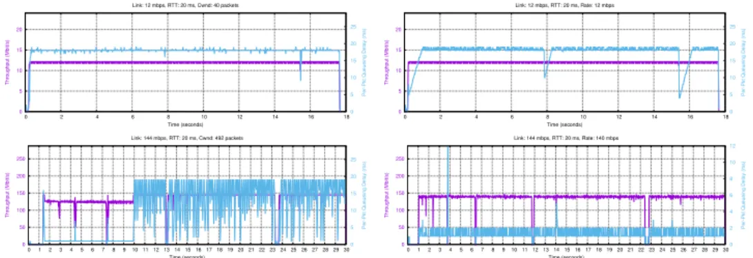
Figure 4-1: Behavior of single flow setting a constant window or pacing rate at a low and high bandwidth. At higher bandwidths, the QUIC cannot sustain the sending rate perfectly and the delays vary more.

As Figure 4-1 shows, as the link rate increases, QUIC cannot maintain the given con-gestion window or pacing rate with the proper queueing delay.1 For all cases, the queueing

delay average should be at most 1 RTT. The sender becomes bursty, and the queueing delay becomes higher and more variable.

4.2.2

Scalability

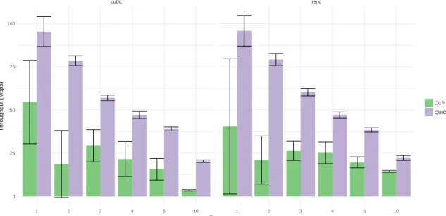
Figure 4-2: Aggregate throughput of an increasing number of flows on a localhost connec-tion. The server runs Reno or Cubic, with and without CCP, and transfers a file of size 100MB to an increasing number of clients. Aggregate throughput is calculated as the total number of bytes transferred to all clients, divided by the maximum file transfer time of any client, averaged across 5 trials. Note that for both CCP and QUIC, aggregate throughput decreases as the number of flows increase. CCP does seem to have slightly lower through-put.

The implementation, with or without CCP, does not scale well as the number of flows increases, in Figure 4-2. This experiment measures the total achieved throughput on local-host as the number of flows increase. The toy client connects to the server over locallocal-host, and measures the time taken to transfer a 100MB file. Here, for each number of flows, ag-gregate throughput is defined as the total amount of data transferred to all clients, divided by the time it took the server to finish the last request for the last client. This value should scale linearly as the number of clients increase; however, the QUIC toy server cannot sus-tain an increasing number of clients. As the number of flows increases, the total achieved

that analyzes either the uplink or downlink logfile from a connection. We use the modified Mahimahi

throughput by all the clients decreases. In addition, for 1 flow, the total achieved through-put on localhost is around 180 mbps; the toy server comes nowhere close to saturating the localhost connection.

CCP Reno and Cubic seem to impose some overhead, as they achieve less throughput than the QUIC toy server. Investigating this overhead remains an area of future work; this performance may be related to the CPU utilization profiles of QUIC alone, and CCP on top of QUIC. CCP mostly sees a decrease in aggregate throughput as well, though not as steep as QUIC’s.

Problems with the QUIC Toy server are well known in previous literature [17].2 This evaluation, as a result, focuses on the similarity of algorithm behavior between QUIC and CCP, as well as the expressiveness of the CCP API.

4.3

Single Flow Behavior

An ideal CCP datapath would produce algorithm implementations that behave exactly as if these algorithms had been implemented natively on the datapath. We examine conges-tion window evoluconges-tion as well as throughput and delay achieved for single clients running QUIC Reno or CCP Reno, and QUIC Cubic or CCP Cubic, on various emulated network conditions. We also discuss BBR, but omit congestion window evolution graphs while dis-cussing BBR. BBR only uses congestion windows to provide a cap on the sending rate; the algorithm dynamics depend heavily on how the pacing rate is set. The experiments cover fixed link, cellular link, and lossy link settings. Each network is emulated with the following parameters:

• One way propagation delay of either 10 ms or 50 ms (DelayShell) • Link trace that either models a constant bandwidth, or a cellular trace3 • Droptail buffer (only for cellular and fixed links):

2_{After further communication with the Google team, we confirmed that the toy server is not optimized for}

performance. The release even states that this server is mainly used for integration test purposes.

– Fixed link: 1 BDP of buffering for TCP Cubic and Reno, and 2 BDPs of buffer-ing for BBR

– Cellular link: 100 packets of buffering (for all three algorithms)

• Deterministic losses: To test lossy links, we add a shell that drops packets at a rate of %.01. The default loss shell in Mahimahi drops packets randomly; to observe how the QUIC and CCP implementations behave in reaction to the exactly same scenario, we modify this shell perform determinstic drops instead. To focus on these determinstic drops and avoid congestive loss, we also emulate infinite buffers.

4.3.1

TCP Reno and TCP Cubic

TCP Reno and Cubic rely on packet loss as a signal for congestion. Reno increases the congestion window linearly, by approximately one packet per RTT, while Cubic uses a cubic function to control congestion window increase. On observing a packet loss, which may or may not have been caused by congestion, a Reno or Cubic sender would reduce the congestion window, usually by 1/2. In the case of a single fixed link with a droptail queue, a sender should see a packet loss approximately when the congestion window hits the sum of the bandwidth delay product and buffersize.

QUIC’s implementation of Reno and Cubic includes two notable differences that would make the behavior diverge from a normal implementation of either algorithm. QUIC, by de-fault, implements a variation on mulTCP in its default TCP congestion control implemen-tation, causing it to emulate two connections rather for a single real connection. QUIC is useful for video playback, so audio and video streams are sent separately over two streams in a QUIC connection. It also uses a different backoff factor: 0.7, instead of 0.5. This results in a different window reduction on losses - instead of cutting the window by half on loss, QUIC cuts the window approximately by .85.4 _{In addition, QUIC uses an alternate}

version of slow start, called Hybrid Slow Start. Hybrid Slow Start uses increasing delay as

4_{The backoff factor in QUIC is calculated by the following equation:}

num_connections − 1 + backoff 2

25 50 75 0 5 10 15 Time (s) Congestion Windo w (Pkts) CCP QUIC

(a) TCP Reno, Fixed 12 MBPS link, 10 ms propagation delay 40 80 120 160 0 10 20 30 Time (s) Congestion Windo w (Pkts) CCP QUIC

(b) TCP Reno, Fixed 24 MBPS link, 10 ms propagation delay 0 200 400 600 0 10 20 30 40 Time (s) Congestion Windo w (Pkts) CCP QUIC

(c) TCP Reno, Fixed 24 MBPS link, 50 ms propagation delay 0 500 1000 1500 2000 0 10 20 30 40 50 Time (s) Congestion Windo w (Pkts) CCP QUIC

(d) TCP Reno, Fixed 48 MBPS link, 50 ms propagation delay 0 200 400 600 0.0 2.5 5.0 7.5 Time (s) Congestion Windo w (Pkts) CCP QUIC

(e) TCP Reno, Lossy 48 Mbps link, 10 ms propagation delay 0 50 100 150 200 0 10 20 30 40 50 Time (s) Congestion Windo w (Pkts) CCP QUIC

(f) TCP Reno, Verizon LTE cellular trace, 10 ms propagation delay

Figure 4-3: Congestion window dynamics of a single TCP Reno flow in various emulated environments. For most cases, the CCP Implementation of TCP Reno seems to follow the congestion window of QUIC Reno quite closely.

a signal to leave slow start early. As QUIC behaves more aggressively, we modify the CCP implementation of Reno and Cubic to use .85 to reduce the congestion window after seeing a loss, in order to provide a fair evaluation.

Figures 4-3 and 4-4 show the congestion window evolution of Reno and Cubic over a six emulated scenarios, and Figure 4-5 shows the throughput and queuing delay achieved for some of the fixed link scenarios. For Reno, the congestion window evolution matches almost perfectly for the lower bandwidth and delay cases in Figures 4-3a and 4-3b. As the BDP of the network increases, for the 24 Mbps or 48 Mbps case with a 100 ms RTT in Figures 4-3c and 4-3d, both QUIC and CCP Reno take longer to exit slow start; this might

20 40 60 0 5 10 15 Time (s) Congestion Windo w (Pkts) CCP QUIC

(a) TCP Cubic, Fixed 12 MBPS link, 10 ms propagation delay 50 100 150 0 10 20 30 Time (s) Congestion Windo w (Pkts) CCP QUIC

(b) TCP Cubic, Fixed 24 MBPS link, 10 ms propagation delay 0 200 400 600 0 10 20 30 Time (s) Congestion Windo w (Pkts) CCP QUIC

(c) TCP Cubic, Fixed 24 MBPS link, 50 ms propagation delay 0 500 1000 1500 0 10 20 Time (s) Congestion Windo w (Pkts) CCP QUIC

(d) TCP Cubic, Fixed 48 MBPS link, 50 ms propagation delay 0 200 400 600 800 0.0 2.5 5.0 7.5 Time (s) Congestion Windo w (Pkts) CCP QUIC

(e) TCP Cubic, Lossy 48 Mbps link, 10 ms propagation delay 0 100 200 0 10 20 30 40 50 Time (s) Congestion Windo w (Pkts) CCP QUIC

(f) TCP Cubic, Verizon LTE cellular trace, 10 ms propagation delay

Figure 4-4: Congestion window dynamics of a single TCP Cubic flow in various emulated environments. For most cases, the CCP Implementation of TCP Cubic seems to follow the congestion window of QUIC Cubic quite closely.

be related to the performance limits of the QUIC server. Figure 4-5c shows that it takes the sender 2 seconds in the 48 Mbps case to fully utilize the link. In the lossy and cellular networks, shown by Figures 4-3e and 4-3f, QUIC Reno exits slow start at a “safer” point and keeps the congestion window lower - while CCP keeps a high congestion window and does not exhibit clear Reno-like behavior. The CCP Cubic implementation behaves more normally in terms of slow start, in the scenarios shown. The differences in the Cubic results may come from implementation choices in QUIC; the CCP Cubic evolution shows more of a cubic increase than QUIC. In Section 5.1, we discuss implementing Hybrid Slow Start inside CCP and show that this implementation more faithfully emulates QUIC’s TCP Reno

0 5 10 15 20 0 2 4 6 8 10 12 14 16 18 0 5 10 15 20 25 Throughput (Mbit/s)

Per-Pkt Queueing Delay (ms)

Time (seconds) Fixed, BW: 12, Delay: 10, Alg: ccp cubic, Filesize: 25MB, Trial: 1

sum

(a) TCP Cubic in CCP QUIC, Fixed 12 MBPS link, 10 ms propagation delay

0 5 10 15 20 0 2 4 6 8 10 12 14 16 18 0 5 10 15 20 25 Throughput (Mbit/s)

Per-Pkt Queueing Delay (ms)

Time (seconds) Fixed, BW: 12, Delay: 10, Alg: cubic, Filesize: 25MB, Trial: 1

sum

(b) TCP Cubic in native QUIC, Fixed 12 MBPS link, 10 ms propagation delay

0 10 20 30 40 50 60 70 80 90 0 2 4 6 8 10 12 14 16 18 20 0 5 10 15 20 25 Throughput (Mbit/s)

Per-Pkt Queueing Delay (ms)

Time (seconds) Fixed, BW: 48, Delay: 10, Alg: ccp reno, Filesize: 50MB, Trial: 1

sum

(c) TCP Reno in CCP QUIC, Fixed 48 MBPS link, 10 ms propagation delay

0 10 20 30 40 50 60 70 80 90 0 2 4 6 8 10 12 14 16 18 20 0 5 10 15 20 25 Throughput (Mbit/s)

Per-Pkt Queueing Delay (ms)

Time (seconds) Fixed, BW: 48, Delay: 10, Alg: reno, Filesize: 50MB, Trial: 1

sum

(d) TCP Reno in Native QUIC, Fixed 48 MBPS link, 10 ms propagation delay

Figure 4-5: Downlink throughput and queueing delay for TCP Cubic and Reno over a fixed bandwidth link. The left side shows CCP, while the right side shows QUIC.

and TCP Cubic.

4.3.2

BBR

Per-Pkt Queueing Delay (ms)

Time (seconds) Fixed, BW: 12, Delay: 10, Alg: ccp bbr, Filesize: 25MB, Trial: 1

sum

(a) BBR in CCP QUIC, Fixed 12 MBPS link, 10 ms propagation delay

0 5 10 15 20 0 2 4 6 8 10 12 14 16 18 0 5 10 15 20 25 30 35 40 Throughput (Mbit/s)

Per-Pkt Queueing Delay (ms)

Time (seconds) Fixed, BW: 12, Delay: 10, Alg: bbr, Filesize: 25MB, Trial: 1

sum

(b) TCP BBR in native QUIC, Fixed 12 MBPS link, 10 ms propagation delay

Figure 4-6: Downlink throughput and queueing delay for BBR and QUIC BBR flow. BBR [6, 7], introduced by Google in 2016, is an alternate to loss based congestion control. A BBR sender estimates the rate of packets delivered to the receiver, and sets its sending rate to the maximum delivered rate (over a sliding time window), which is believed to be the rate of the bottleneck link between the sender and the receiver. To determine whether a connection can send more than its current rate estimate, it probes the link for additional bandwidth by temporarily increasing its rate by a factor of 1.25. In order to drain the queue that may have been created in response to the rate increase, it then reduces its

rate to 0.75 of the rate estimate, before sending at its new estimate bottleneck rate estimate. On a fixed link, it would ramp up to the correct bandwidth and remain there for the rest of the connection. The BBR sender also drains the queues (by reducing the congestion window to 4) periodically, in order to get a new accurate measurement of theminrttof the link. Figure 4-6 shows that on a fixed link (12 Mbps), both BBR implementations drain the queue about every 10 seconds to redetermine the minrtt. In the steady state, both sustain about 12 Mbps. Note that the CCP implementation of BBR5 only includes the PROBE_BW

andPROBE_RTTphases. It remains future work to implement theSTARTUPandDRAINphases, as well as the special policing detection the full BBR implementation includes. The CCP QUIC implementation of BBR experiences similar delays, but does not match QUIC BBR on startup. Investigating the startup behavior remains future work.

4.3.3

Summary

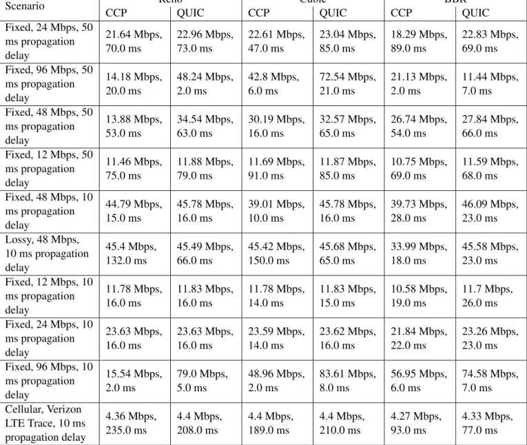
Table 4.1 summarizes the fidelity results for comparing single flows of Reno, Cubic and BBR between their CCP and native QUIC versions. The utilized throughput and queueing delay in each case is measured via Mahimahi logs.

4.4

Request Completion Times

QUIC is typically used to serve data over HTTP - a natural metric is to benchmark how fast various congestion control algorithms can transfer various files from the client to a server. Figure 4-7 summarizes file transfer speed in Cubic, Reno and BBR with and without CCP across cellular, fixed and lossy link cases. For the fixed link case, we run each algorithm on a 48 MBPS link with a 10 ms one way propagation delay; the lossy shell experiments add deterministic drops at the rate of .01%. For the cellular link case, we use the Verizon LTE trace used previously in Section 4.3. CCP versions of algorithms are slightly slower at completing the file transfer requests.

Scenario Reno Cubic BBR

CCP QUIC CCP QUIC CCP QUIC

Fixed, 24 Mbps, 50 ms propagation delay 21.64 Mbps, 70.0 ms 22.96 Mbps, 73.0 ms 22.61 Mbps, 47.0 ms 23.04 Mbps, 85.0 ms 18.29 Mbps, 89.0 ms 22.83 Mbps, 69.0 ms Fixed, 96 Mbps, 50 ms propagation delay 14.18 Mbps, 20.0 ms 48.24 Mbps, 2.0 ms 42.8 Mbps, 6.0 ms 72.54 Mbps, 21.0 ms 21.13 Mbps, 2.0 ms 11.44 Mbps, 7.0 ms Fixed, 48 Mbps, 50 ms propagation delay 13.88 Mbps, 53.0 ms 34.54 Mbps, 63.0 ms 30.19 Mbps, 16.0 ms 32.57 Mbps, 65.0 ms 26.74 Mbps, 54.0 ms 27.84 Mbps, 66.0 ms Fixed, 12 Mbps, 50 ms propagation delay 11.46 Mbps, 75.0 ms 11.88 Mbps, 79.0 ms 11.69 Mbps, 91.0 ms 11.87 Mbps, 85.0 ms 10.75 Mbps, 69.0 ms 11.59 Mbps, 68.0 ms Fixed, 48 Mbps, 10 ms propagation delay 44.79 Mbps, 15.0 ms 45.78 Mbps, 16.0 ms 39.01 Mbps, 10.0 ms 45.78 Mbps, 16.0 ms 39.73 Mbps, 28.0 ms 46.09 Mbps, 23.0 ms Lossy, 48 Mbps, 10 ms propagation delay 45.4 Mbps, 132.0 ms 45.49 Mbps, 66.0 ms 45.42 Mbps, 150.0 ms 45.68 Mbps, 65.0 ms 33.99 Mbps, 18.0 ms 45.58 Mbps, 23.0 ms Fixed, 12 Mbps, 10 ms propagation delay 11.78 Mbps, 16.0 ms 11.83 Mbps, 16.0 ms 11.78 Mbps, 14.0 ms 11.83 Mbps, 15.0 ms 10.58 Mbps, 19.0 ms 11.7 Mbps, 26.0 ms Fixed, 24 Mbps, 10 ms propagation delay 23.63 Mbps, 16.0 ms 23.63 Mbps, 16.0 ms 23.59 Mbps, 14.0 ms 23.62 Mbps, 16.0 ms 21.84 Mbps, 22.0 ms 23.26 Mbps, 23.0 ms Fixed, 96 Mbps, 10 ms propagation delay 15.54 Mbps, 2.0 ms 79.0 Mbps, 5.0 ms 48.96 Mbps, 2.0 ms 83.61 Mbps, 8.0 ms 56.95 Mbps, 6.0 ms 74.58 Mbps, 7.0 ms Cellular, Verizon LTE Trace, 10 ms propagation delay 4.36 Mbps, 235.0 ms 4.4 Mbps, 208.0 ms 4.4 Mbps, 189.0 ms 4.4 Mbps, 210.0 ms 4.27 Mbps, 93.0 ms 4.33 Mbps, 77.0 ms

Table 4.1: Throughput and delay achieved in various fixed, cellular, and lossy scenarios for CCP QUIC and QUIC Reno, Cubic and BBR flows. The lossy shells add .01% de-terministic drops. The capacity of the Verizon trace varies over time, but is 4.5 Mbps on average.

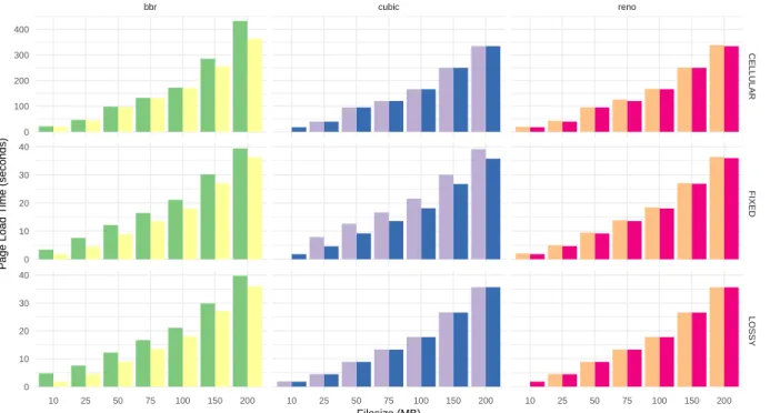
bbr cubic reno CELLULAR FIXED LOSSY 10 25 50 75 100 150 200 10 25 50 75 100 150 200 10 25 50 75 100 150 200 0 100 200 300 400 0 10 20 30 40 0 10 20 30 40 Filesize (MB) P

age Load Time (seconds)

CCP BBR CCP Cubic CCP Reno QUIC BBR QUIC Cubic QUIC Reno

Figure 4-7: Request completion times for a 100 MB file across Cubic, Reno and BBR for fixed (48 Mbps, 20 ms RTT), lossy (48 Mbps, 20 Ms RTT, .01% deterministic drops) and cellular (Verizon uplink trace, 20 ms RTT) environments. Cubic and Reno match almost perfectly for lossy and cellular environments and are slightly slower in the fixed link environment. The CCP version of BBR is slightly slower; this may be attributed to the different startup behavior shown in Figure 4-6.

4.5

Multiple Flow Behavior

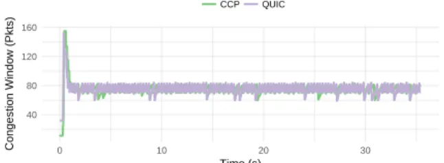
Two TCP Cubic or Reno flows should share a link fairly and each get about half the band-width of the link. This section evaluates whether the CCP version of Cubic on QUIC behaves similarly to native QUIC with respect to the behavior of multiple cubic flows. Fig-ure 4-12 reveals that two CCP QUIC flows and 2 QUIC flows share the link equally. At three flows, QUIC continues to share the link equally, while the performance degrades for two out of the three CCP flows. This may be related to the performance degradation seen for multiple clients seen on localhost for CCP QUIC, discussed in Section 4.2. Note that this experiment only shows one run; when multiple CCP flows are involved, the variation is extremely high.

0 10 20 30 40 50 60 70 80 90 0 2 4 6 8 10 12 14 16 18 20 0 5 10 15 20 Throughput (Mbit/s)

Per-Pkt Queueing Delay (ms)

Time (seconds)

sum 54966 59892

Figure 4-8: 2 CCP Cubic flows: 20.69 and 20.56 Mbps 0 10 20 30 40 50 60 70 80 90 0 2 4 6 8 10 12 14 16 18 20 0 5 10 15 20 25 Throughput (Mbit/s)

Per-Pkt Queueing Delay (ms)

Time (seconds)

sum 44124 52628

Figure 4-9: 2 QUIC Cubic Flows: 21.94 and 21.92 Mbps 0 10 20 30 40 50 60 70 80 90 0 1 2 3 4 5 6 7 8 9 10 11 12 13 14 15 16 17 18 19 20 21 22 23 24 25 26 27 28 29 30 31 32 33 34 35 0 5 10 15 20 25 Throughput (Mbit/s)

Per-Pkt Queueing Delay (ms)

Time (seconds)

sum 52903 34691 34105

Figure 4-10: 3 CCP Cubic Flows: 14.88 Mbps, 11.94 Mbps, 11.513 Mbps 0 10 20 30 40 50 60 70 80 90 0 1 2 3 4 5 6 7 8 9 10 11 12 13 14 15 16 17 18 19 20 21 22 23 24 0 5 10 15 20 25 Throughput (Mbit/s)

Per-Pkt Queueing Delay (ms)

Time (seconds)

sum 40209 39038 46566

Figure 4-11: 3 QUIC Cubic Flows: 16.81 Mbps, 16.69 Mbps, 16.72 Mbps

Figure 4-12: Throughput and queueing delay of multiple Cubic flows on a fixed link with 48 mbps bandwidth and 10 ms propagation delay.

4.6

Discussion

These results reveal that CCP faithfully implements congestion control for Reno, Cubic and BBR over QUIC, with a slight overhead in terms of performance. While the congestion window graphs show that CCP Cubic and Reno implementations do not match exactly with their native QUIC counterparts, we believe that these differences are due to modifications made to the TCP algorithms inside QUIC. The different implementations of slow start between CCP and QUIC led to some of the differences in the various emulated networks, especially in the cellular cases. Section 5.1 discusses implementing Hybrid Slow Start in CCP to evaluate whether the CCP API provides as much flexibility as the QUIC pluggable congestion control interface and if the fidelity results improve.

Future work includes a more throrough investigation of the scalability results seen by CCP QUIC; since the QUIC toy server itself is limited in performance, it is difficult to isolate the performance overhead of CCP. Ideally, in the future, we can even implement CCP for high performing QUIC server.

Chapter 5

Writing Algorithms in CCP

This section discusses the CCP API, as well as CCP’s ability to allow “write once, run anywhere” behavior. By “API”, we refer to the congestion control functionality available for users to write algorithms: the set of congestion signals available for summarizing in datapath programs as well as the operations allowed over those signals. Currently, pacing rates and congestion windows are the only ways datapaths enforce sending rates. Since CCP supports both pacing rates and windows, we focus on evaluating the expressiveness of the datapath programs.

We discuss the process of implementing two algorithms using CCP: Hybrid Slow Start [15], an alternate version of slow start, as well as Remy [26], a machine-synthesized congestion control protocol. Ultimately, CCP in its current form cannot supprt Hybrid Slow Start, without modifications to either the algorithm or the CCP API. The CCP API supports the requirements for implementing Remy, but we find that further work is required to optimize the performance of the algorithm. Finally, a primary motivating factor in building CCP is automatically allowing various algorithms to be run on multiple datapaths. We show in-stances of the exact same implementation of various algorithms exhibiting similar behavior in various datapaths.

5.1

Hybrid Slow Start

Hybrid Slow Start uses increasing delay as a signal to end slow start and enter the con-gestion avoidance phase. QUIC’s pluggable concon-gestion control interface provides Hybrid Slow Start as a module to incorporate into TCP based algorithms; the evaluation of Hybrid Slow Start in CCP QUIC involves comparing with QUIC’s implementation of Hybrid Slow Start.1

5.1.1

Algorithm

Hybrid Slow Start [15] attempts to solve the problem of regular TCP slow start causing a large number of packet losses towards the beginning of a connection, due to the fast congestion window increase of doubling the window per ACK. While this allows a sender to probe the link for the available bandwidth, due to large buffers within the network, the sender may overshoot its congestion window estimate by a large amount.

In Hybrid Slow Start, the sender still increases its congestion window exponentially, but does not wait for a loss or timeout event to exit slow start. Rather, the sender uses ACK train length and packet delay increase a signal to leave slow start earlier. The QUIC implementation only includes the packet delay increase measurement; ACK train length detection may interfere with packet pacing. As a result, within CCP, we only implement delay increase detection.

The sender keeps track of rounds of packets approximately every RTT. A round is defined by a burst of packets the sender sends together; once the sender receives ACKs for the last packet in the previous burst it sent, the round is considered over. Within each RTT round, it keeps track of the minimum RTT of the first 8 packets received. At each round, it checks whether the current round’s minimum RTT is too high - specifically, the sender sees whether the current round’s minimum RTT is above the sum of the total minimum RTT of the link plus a threshold. If the current round’s minimum RTT is too high, the sender leaves slow start, sets ssthresh to be the current congestion window and enters the

1_{Our implementation is located athttps://github.com/ccp-project/portus/blob/hystart/ccp_generic_}

congestion avoidance phase.

5.1.2

Implementation in CCP

6 (:= currentMinRtt (min currentMinRtt Flow.rtt_sample_us))

7 (fallthrough) 8 ) 9 (when (== rttSampleCount 8) 10 (:= minRttIncreaseThreshold (/ minrtt 8)) 11 (fallthrough) 12 )

13 (when (&& (> minRttIncreaseThreshold 0) (&& (> Cwnd 16) (> currentMinRtt (+ minrtt minRttIncreaseThreshold))))

14 (report)

15 )

16 (when (|| (> Ack.last_acked roundEnd) (== Ack.last_acked roundEnd))

17 (:= currentMinRtt +infinity)

18 (:= rttSampleCount 0)

19 (:= roundEnd Ack.last_sent)

20 (fallthrough)

21 )

Figure 5-1: Excerpt of Hybrid Slow Start implemented with new congestion signals that expose which sequence number is last acked, as well as which sequence number was last sent. We omit the program variable definitions and only show the conditions to leave slow start.

Since CCP provides RTT as a congestion signal, a datapath program should be able to measure delay increase quite easily and compare this increase to a threshold value. How-ever, it is unclear how to demarcate “rounds” of packet bursts using the CCP API. The QUIC pluggable congestion control API provides a callback when packets are sent - us-ing this callback, the QUIC sender keeps track of the sequence number of the last packet sent. At the beginning of each send round for Hybrid Slow Start, it marks the end of the round as the last packet sent. On each ACK, the sender checks if it has received the ACK corresponding to the end of the round; if so, the send round is over.

1 (when (> Micros minrtt) 2 (:= currentMinRtt +infinity) 3 (:= rttSampleCount 0) 4 (:= Micros 0) 5 (fallthrough) 6 )

Figure 5-2: Excerpt of Hybrid Slow Start implemented where packet rounds end on each minimum RTT.

CCP, on the other hand, does not expose information about specific sequence numbers sent or received. CCP aims to expose a more general congestion control protocol API -sequence numbers may imply the transport is TCP based; CCP could support UDP or TCP based datapaths. Instead of sequence numbers, CCP datapaths expose the amount of new bytes and packets everytimeccp_invokeis called. Within CCP, we could approximate when sending rounds start by using the global minimum RTT of the connection. Each round of packets takes about one RTT to be received. However, this approximation is not ideal, as ACK compression or delayed ACKs could delay the time a burst of packets has been fully received. Another approach involves observing the ACK interarrival times - if the ACK interarrival time increases by a large amount, the new ACK is probably from a new burst of packets. This approach is not ideal because other issues in the network, such as congestive or non congestive packet loss, could cause this estimate to be less accurate.

In this experiment, we implement two variations of the delay increase portion of Hybrid Slow Start in CCP:

1. In the first, we modify the QUIC datapath to mark both the sequence number of the last sent packet using the OnPacketSent()callback, as well as the the sequence number of the current packet being acked. Note that in the QUIC CCP datapath, datapath programs are updated everytime ccp_invoke is called, which happens per ACK in QUIC. The CCP then provides both of these variables for use in the dat-apath programs. The datdat-apath program, shown in Figure 5-1, then marks when rounds start and end using these new congestion signal primitives (Ack.last_sent