Analysis of the performance of the buried pipe grid of a heat pump

Publisher’s version / Version de l'éditeur:

Vous avez des questions? Nous pouvons vous aider. Pour communiquer directement avec un auteur, consultez la

première page de la revue dans laquelle son article a été publié afin de trouver ses coordonnées. Si vous n’arrivez pas à les repérer, communiquez avec nous à PublicationsArchive-ArchivesPublications@nrc-cnrc.gc.ca.

Questions? Contact the NRC Publications Archive team at

PublicationsArchive-ArchivesPublications@nrc-cnrc.gc.ca. If you wish to email the authors directly, please see the first page of the publication for their contact information.

https://publications-cnrc.canada.ca/fra/droits

L’accès à ce site Web et l’utilisation de son contenu sont assujettis aux conditions présentées dans le site LISEZ CES CONDITIONS ATTENTIVEMENT AVANT D’UTILISER CE SITE WEB.

Internal Report (National Research Council of Canada. Division of Building Research), 1957-09-01

READ THESE TERMS AND CONDITIONS CAREFULLY BEFORE USING THIS WEBSITE.

https://nrc-publications.canada.ca/eng/copyright

NRC Publications Archive Record / Notice des Archives des publications du CNRC :

https://nrc-publications.canada.ca/eng/view/object/?id=012741d0-50e5-4990-bad1-56b638a0577a https://publications-cnrc.canada.ca/fra/voir/objet/?id=012741d0-50e5-4990-bad1-56b638a0577a

For the publisher’s version, please access the DOI link below./ Pour consulter la version de l’éditeur, utilisez le lien DOI ci-dessous.

https://doi.org/10.4224/20386683

Access and use of this website and the material on it are subject to the Terms and Conditions set forth at

Analysis of the performance of the buried pipe grid of a heat pump Brown, W. G.

DIVISION OF BUILDING RESEARCH

ANALYSIS OF THE PERFORMANCE OF THE BURIED PIPE GRID OF A HEAT PUMP

by

W.G. Brown

Report No. 129 of the

Division of Building Research

OTTAWA September, 1957

Interest in the possible uses of equipment operating on the reversed refrigeration cycle, more commonly known as heat pumps, developed rapidly following the end of the

war in 1945. It was believed by many that such equipment

would find extensive use in space heating. Several Divisions

of the National Research Council had an interest in these possibilities and it was finally agreed that the Division

of Building Research should investigate them. Compressor

equipment already available for this work was turned over to the Division and planning of the project was begun. The ground coil was selected as the heat source for study.

Before experimental work was begun the Division invited representatives from other Divisions, several interested university departments, refrigeration

manufac-ｴｾｲ･ｲｳ and the Hydro-Electric Power Commission of Ontario, to meet as a Heat Pump Committee and to give the benefit

of their thinking and experience to the project. This

Committee met first in 1949 and again in 1952.

Progress on the project was slow for several reasons, including equipment difficulties, and the need for changes in the experimental procedures and immediate objectives which were indicated as experience was gained

in the work. As a result, no extensive test program

was carried out before it became necessary to reconsider complete replacement of the compressor eqUipment and

reconstruction of the ground coil at a new site. When,

at this stage, the project was reconsidered in relation

to other important commitments of the Division, the decision was made, with regret, to discontinue experimental work

until some future date.

The operating results obtained from numerous

experimental runs made over two years have now been analysed. This analysis, together with the conclusions drawn from the

experimental data are now presented. Specific portions of

the work and the eqUipment used have been described in undergraduate theses prepared by two students who were

employed in summer work on the project. The records of

the two meetings of the Committee are contained in the Proceedings which have been issued.

The experience gained in this project, some of which still remains to be reported, indicates not so much any lack of technical feasibility of the heat pump, as it does the difficulty in dealing on a proper experimental basis with thermal problems involving the ground.

Ottawa

PIPE GRID OF Aｈｒｾｔ ｰｵｲｮ［ｾ

by W.G. Brown

INTRODUCTION

In recent years considerable interest has arisen in Canada over the possibility of heating and cooling

buildings by means of the heat. pump. This interest has

been due mainly to successful applications in the United States, particularly in the South.

The heat pump ｾｳ a refrigeration system in which

heat is extracted at low temperature from an external

source and discharged at high temperature. For cooling

purposes the cycle can be reversed. The advantage of the

heat pump is that, generally, the heat supplied is two or more times as much as the electrical heat eqUivalent

of the compressor motor power. The magnitude of this

advantage, however, decreases as the difference between the heat discharge and extraction temperatures increases.

In southern regions two factors have combined to

favour the heat pump: the availability of heat sources

at relatively high temperatures results in correspondingly low operating costs for winter heating; and summer cooling loads, being large, require equipment of capacity similar

to that for the heating load. Summer air-conditioning is

being regarded more and more as a necessity in northern parts of the United States, and where it is required the high initial costs of the heat pump can be justified.

In

Canada, climatic conditions are considerably different

from those in the South; winter heating requirements are greater while summer cooling loads are generally lower.

Under these conditions a heat pump would not be as effective as in warmer climates but still may be feasible when both heating and cooling are required.

Natural heat sources in Canada, (air, water or

ground) are available only at comparatively low

tempera-tures when winter heating requirements are greatest. Since

the feasibility of a heat pump installation may depend strongly on the quality of the source it is important to be able to predict the source characteristics accurately. Although air is the most accessible source it has two

serious disadvantages in cold climates: its temperature

is the lowest of the natural sources and; there is danger of evaporator coil frosting at times of greatest heat demand. Water is not usually available, hence for most potential

heat pump installations the ground would serve as the

heat source. As a step in investigating the possibilities

of the heat pump in Oanada, a project to study the ground heat source was instituted in 1949 by the Division of Building Research of the National Research Oouncil.

The performance theory for pipes buried in the

ground (I) has beerravailable for many years. In general,

however, this theory has been developed for idealized conditions and has not had extensive experimental

verifi-cation, particularly for long-term operation. Among the

factors usually neglected in theoretical calculations are the effects of soil freezing and temperature-induced

moisture migration, variable soil thermal properties due to non-uniform moisture distribution, and non-uniform heat extraction rates due to fluctuating heating demands. In addition, design calculations usually assume long-term or steady-state operation at the maximum heat extraction rate, whereas in reality the performance depends on the

previous history of heat extraction. Under these conditions

a ground grid designed theoretically may be oversized. This report deals with these factors and their importance by comparing observed and calculated data during a full season of heating operation and by comparison of prior history-dependent operation with steady-state operation.

BQUIPMENT AND PROOEDURE

The Heat Pump

The heat pump used in conjunction with the

investi-gationof the buried pipe grid consisted of 3 Brown-Boveri

compressors of Ｒｾ hp each which could be connected in

parallel. The refrigerant, (Freon 12) was circulated

through 3 heat exchangers (evaporators), where heat was

extracted from the secondary refrigerant of the ground

pipes. The condenser consisted of a forced air Freon heat

exchanger.

The Ground Gri d

The ground pipe grid (Fig. 1) consisted of 5 parallel loops of I-in. copper pipe (1.125 in. O.D.) approximately 189 ft long, on 5-ft centres and buried 6

ft deep. The loops were connected to common supply and

return headers and, by means of shut-off valves, could be used in any parallel combination., All pipes connecting the grid and the headers were insulated to reduce heat

transfer ｢･ｾｎ･･ｮ supply and return refrigerant. The

refrigerant circulated in the pipes was calcium chloride brine having specific gravity 1.21 and specific heat 0.71.

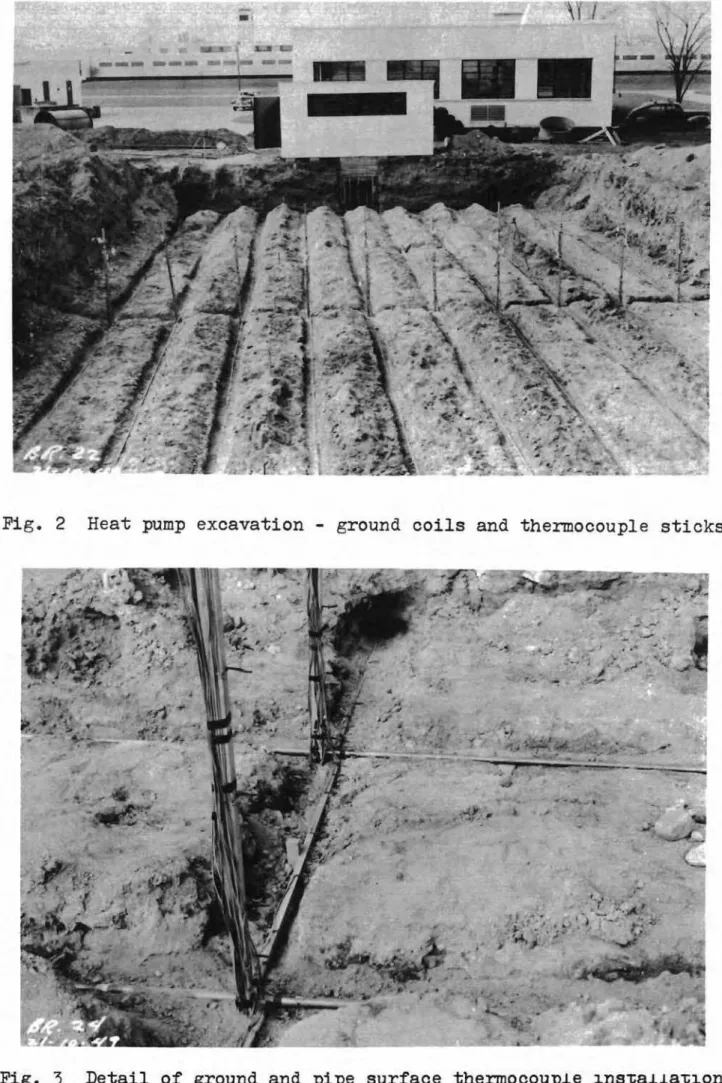
The original soil at the grid site was mainly sand,

thus sand was used to back-fill the 54- by 100-ft excavation

to give the best possible soil uniformity. The completed

excavation with the pipes in place prior to back-filling is shown in Fig. 2.

About 200 thermocouples, (20 gauge copper-constan-tan with neoprene insulation and a waterproof cover), were installed to measure pipe surface, brine, and surrounding

ground tanperatures. Pipe surface thermocouples were

sol-dered in place at the middle of each supply and return run

and also at 15-ft intervals along the middle loop, (loop 0).

Brine thermocouples were placed in wells at the beginning

and end of eaoh loop. Ground thermocouples, supported

by wooden sticks, were installed vertically and horizontally,

i,

!,

1 and 2 ft from the centre-line at the middle of

each pipe run. Additional ground thermocouples were installed

at the same location at depths of 1, 3 and about 9 ft below the ground surface, (bed-rock was encountered about

9 ft deep). Thermocouples were also installed at horizontal

distances of

4

and 6 ft beyond the outermost pipes.

Installation details are shown in Fig. 3. Measurements

Ground and pipe surface temperatures were measured on a self-balancing potentiometer indicator (sensitivity O.IOF) and brine temperatures were recorded on a

multi-point recorder, (accuracy approx. 1°F). Brine flow rates,

(6 to 20 gal/min) were measured with a calibrated volumetric

displacement meter. Heat extraction rates were calculated

from the temperature increases along the pipe and the brine

flow rates. Differential pressures across 5/S-in. orifices

in each pipe loop were equalized to ensure identical brine

flow rates. In conjunction with operation of the pipe grid,

several samples of soil were analysed for density, moisture content and grain size distribution.

Scope of Tests and Analysis of Data

The data for the experimental investigation were obtained in three stages:

(1) Preliminary tests

TV/o short-term tests of 2- and 3-days' duration

were made in July 1950 using pipe loop O. In the analysis

these data were used to determine the thermal conductivity and diffusivity of the ground.

Cp =

(2) Operation during the heating season

From October 1950 to May 1951 the ground grid pipe loops were used in various combinations and heat extraction

rates and pipe surface temperatures were recorded. The

metIlod of analysis of the data for this period consisted of comparing observed pipe surface temperatures at various

times with ｴｨｯｾ･ calculated using the ground properties

determined from the preliminary tests.

(3) Normal ground temperatures

Soil temperatures were recorded for an additional two years after completion of the heat extraction tests to determine normal temperature changes due to the annual

weather cycle. These data were not used in the analysis

but were of interest in illustrating how ground tempera-tures vary with depth and time during the year.

RESULTS AND DISCUSSION

(I) ｐｒｅｌｉｾｲｲｎａｒｙ TESTS - DETERMINATION OF SOI1 THEmvUlL

PROPERTIES Heat Extraction Rates

In the preliminary tests on pipe loop 0, (July

18 to 21 and July 27 to 28, 1950) pipe surface and soil

temperatures were recorded periodically. The heat transfer

rates in B.t.u. per hr per ft of pipe were calculated using the formula,

Ql

= w Cp

AT,

(I)

1

where: w

=

brine flow rate in lb per hr

(5240 for both tests), specific heat of brine

(0.71 B.t.u./hr/oF),

6T

=

temperature rise along the pipe (OF),

1

=

pipe length (189 ft).

During both preliminary tests, the multi-point

temperature recorder was found to be insufficiently accurate for determination of the small rise in brine temperature

along the pipe (0° to 4°F). Calculation showed, however,

that at the brine flow rates used in the tests the tempera-ture difference between the brine and pipe surface would

measured with the more accurate temperature indicator

were used to calculate heat extraction rates. Since this

instrument was read only to the closest ｾｯｆＬ however,

heat extraction rates could not be accurately determined. Although the amounts of heat extracted by the brine during

the July 18 to 21 test (Fig. 4) were uncertain, the

ex-traction rates appeared to increase during the first

several hours warm-up period, then decreased gradually for

the remainder of the test. The gradually decreasing

rates after the initial warm-up period were due to the

method of operation of the primary refrigeration system, (constant superheat, in which heat extraction decreases as the evaporator or heat exchanger temperature decreases). For the first few minutes of operation the heat extraction rates were presumably negative since the brine in the heat exchangers linking the primary and secondary refrigeration systems was initially at ambient temperature, (about 70°F), whereas the ground temperature at the pipe was 59°F.

Pipe Surface Temperatures

Pipe surface temperatures, (Fig. 5) decreased continuously during the July 18 to 21 test from 59°F

initially to 25°P after 5 days' time. Results were similar

for the July 27 to 28 test. In this second test, however,

all temperatures were slightly lower than in the first since the ground and pipe surface temperatures had not

completely recovered in the intervening time between tests.

Determination of the Thermal Pronerties of the Soil_.

Available theory for buried pipes (1) shows that for short-term tests the temperature "decrease" below nor-mal temperature at any radial distance from a pipe including the pipe surface* is given by:

6T I (2 )

where. :AT

=

the "decrease" in temperature below the normal

temperature at the point in question,

Ql

=

the heat extraction rate per unit length of pipe,

k = the thermal conductivity of the soil,

I

=

the line source integral)

(see reference (1) p. 297 for tabulation),

Ｍｉｾ For very short times (less than about 1 hour) the theory

r

=

the radius,

ｾ

=

the thermal diffusivity,

t

=

the time from start of operation.

Equation 2 shows that if Ql, k and ｾ can be assumed

constant as a first approximation then ｾｔ is a function

only of ｾ or t/r2• Consequently, a graph of ｾｔ versus

t

2 should give a single line from which the diffusivity ｾ

r

could be determined using the equation. JThe thermal

conductivity would remain unknown since QL was not accurately

known, )

In this method of comparing temperature "decrease" data for the pipe and various points in the surrounding SOil, the normal soil temperatures at the points in question (Figs. 6 and 7) were assumed to be the same as

those measured at the beginning of the test. This

assump-tion was valid since measurements at unused pipes A and E

showed that the normal temperatures remained essentially unchanged for several days.

Results for pipe surface, 0.25, 0.5 and 1.0 foot

radii, (Figs. 8 and 9) showed the assumptions involved in

using equation 2 werG valid as a first approximation. Using the equation, the thermal diffusivity was found to

be about 0.04 ft 2/hr (see Appendix I for all calculations

of this section).

Although the thermal conductivity could not be determined directly from the test data it was determined indirectly from the moisture content and density data

obtained in conjunction with the tests (Table

I).

This

was possible since thermal conductivity, density, diffusivity and specific heat are related by the formula

k = 0< ;:> Cp,

wherejO is the soil density, and Cp the soil specific heat. Although the specific heat in turn was not measured,

published information (3) shows it can be calculated from the equation:

Cp = 100C + M ,

100 + M

where M is the percentage moisture content and C is the specific heat of dry soil (0.16 to 0.17 B.t.u./lb/oF).

The thermal conductivity obtained by use of these equations was 1.2 B.t.u./hr/oF/ft.

With the conductivity established, equation 2 was then reused to determine the average heat extraction

rate. The value obtained, (61 B.t.u./hr/ft) agreed moderately

well with the apparent mean of the measured heat extraction

rates (Fig. 4).

Although the data of Figs. 8 and 9 for the 0.25-, 0.5- and 1.0-ft radii appeareG to correlate, the data for the pipe surface failed to do so at large values of t/r2• As mentioned preViously, however, the heat-extraction rates were knOVrrl to vary with time, but the form of the relationship was unknown due to measurement inaccuracies. Thus, in order to determine more accurately the ground properties and the form of the heat extraction-time

relationship, further analysis was carried out. The analysis

method consisted of assuming constant heat-extraction rates for short periods of time and using equation 2 to sum the temperature "decreases" at the pipe surface

caused by these rates. By equating this sum to the measured

pipe surface temperature "decrease" the individual

heat-extraction rates could be determined step by step. This

procedure was used for several values of thermal

con-ductivity and diffusivity as related by equation 3. The

heat-extraction rates were determined; then the temperature "decreases" at the various radii in the soil were computed

for comparison with observed values. The best agreement,

(Fig. 10, calculations given in Appendix II) was obtained

for a thermal conductiyity of 0.9 B.t.u./hr/oF/ft and a

diffusivity of 0.03 ｦｴｾＯｨｲＮ The values of heat-extraction

rate determined from the calculations (Fig. 4) were in

good agreement with the apparent measured rates.

There was some minor uncertainty about the values of heat flow, conductivity and diffusivity due to possible

errors in thermocouple positioning (about

t

in.). In

addition, some temperature error was apparent, presumably due to switching errors or imperfect grounding of

eqUip-ment (see 1.0-ft radius at beginning of test in Fig. 10).

ｾｴｩｳ･ｮ･ｲ (2) reports similar difficulties in temperature

measurements and errors of the same magnitudes. The value

of thermal conductivity of 0.9 B.t.u./hr/ft/oF, however,

agrees fairly well with the accepted value of 1.0 B.t.u./hr/ft/oF

for sandy soil (3). The assumption of constant diffusivity

is supported by results of Penrod

(4)

who reports tests

using a heat pump to determine the thermal diffusivity of

a clay-type soil. His results for several days operation

showed a constant diffusivity up to at least 1.5 ft from a buried pipe.

Effect of Soil Freezing and Moisture ｾｵｧｲ｡ｴｩｯｮ

The predominance of large particles in the soil grain-size distribution (Fig. 11) indicates that almost all the moisture present would have been frozen at 32°F.

Published data (3) show that, at the moisture contents present in the tests (Table IB), freezing would not change

the soil thermal properties appreciably. However, the

release of latent heat during the freezing process would cause pipe surface temperatures to be somewhat higher

than with a non-freezing process. Complete theory,

({I) p. 265) is available for the freezing process for

the condition of constant heat extraction rate. The

equations governing are:

[

ｾ ｾ

- k

ｾＨ［

i

T)l ]

e -

ｾ

=

2Lb and

ｉＨｖｾＩ

[

L

I

ＨＲｾ

bT

₌

T - T + -1 0 f _21(k I

(\If )

for r ｾ 2

"!bt

where: T = initial pipe surface temperature

o

Tf = freezing temperature

L = latent heat of fusion per unit volume of soil

b = a constant

Ql

=

heat extraction rate per foot of coil

k = thermal conductivity of soil

ｾ

=

thermal diffusivity of soil

r = pipe radius

t

=

duration of operation

Using these equations and the values of the variables encountered in the July 18 to 21 test, the error in

cal-culated pipe surface temperature due to neglect of freezing was found to be only about O.2°F for any continuous test.

(For calculations see Appendix III.) Calculations by

Ingersoll, Zobel and Ingersoll eel) p. 266) also indicate only small effects due to freezing. ' These authors point

out that, on the basis of equations 4 and

5,

freezing

effects will contribute very little to the performance of a ground coil.

Moisture migration induced by temperature gradients mayor may not have contributed significantly to the heat

extraction. Since the mechanism is not yet fully

under-stood (5), accurate estimates of its effect cannot be

made. In general, however, with moisture migration present

the heat extraction rates would be expected to be higher than without migration due to increased thermal conducti-vity of the soil near tIle pipe and possibly to the latent

heat of condensation of the migrating mcisture. It may be

noted that the theoretical temperature "decreases" (Fig. 10) were too large particularly at the 0.5- and 1.0-ft radii.

If the only effect of moisture migration was to cause a decreasing conductivity gradient from the pipe surface

ｯｵｾｶ｡ｲ､Ｌ then ･ｾｵ｡ｴｩｯｮ 2 shows that the theoretical tempera-ture "decreases' at the 0.5 and 1.0 radii would depart

even more from the observed values. If latent heat effects

were present, however, due to moisture migration in the vapour phase or by alternate condensation and evaporation then only part of the total heat flow in the soil remote from the pipe would take place by conduction and the

remainder would be transmitted by the moisture in the vapour

phase. Near the pipe surface the vapour would condense

and the total heat flow to the pipe would take place only

by conduction in the resulting saturated soil. Under this

condition the pure conduction heat flow would be greater near the pipe than in the remote soil, and the temperature

"decreases" at the 0.5- and 1.0-ft radii would be smaller than those calculated and in better agreement with observed

values. Unfortunately no definite oonclusions can be

drawn about the effects of the moisture migration due to the possibilities of experimental error in the measured

data. The results of the data analysis, however, seem to

indicate that moisture migration was not a significant contributor to the buried pipe performance.

(2 ) OPERATION DURING THE HEATInG SEASON

Procedure and Measurements

From October 1950 to May 1951 the pipe loops were used in various parallel arrangements to study the effect of this type of operation on heat extraction rates and

ground and pipe temperatures. For the first

2t

weeks in

October, pipe

a

was used alone for 7 hours each day,

(excepting week-ends). From November to April operation

was continuous for about 100 hours each week. Beginning

with loop

a,

progressively more pipe loops were added to

the system during this period. During April and May short

tests (3 to 30 hours) were made using the individual pipe

During the heating season all temperatures were

measured twice daily with a precision of O.loF. With

this precision, however, the heat extraction rates calculated from equation 1 still had considerable possible error.

For pipe 0, in which the temperature rise in 189 ft of

pipe was measured, the possible errors would be

4.5

and

1.0 B.t.u./hr/ft of pipe at brine flow rates of 6000 and

1300 lb/hT respectively. The possible error for the other

pipes of the grid would be double these values since temperature rises were measured along only one-half the

pipe length (see Fig. 1). In addition, some of the

thermo-couples along pipe

a

periodically gave erroneous readings

indicating that additional errors may have been present in the measurements on the other pipes which had only two surface thermocouples.

Data Analysis

Since the heat pump was operated arbitrarily the data would be of limited direct use for practical design

purposes. The results of the preliminary tests, however,

indicated that moisture migration effects were probably small and theoretical calculations might be expected to

agree fairly well With observed data. If this could be

established the design procedure for ground pipe grids

could be ｾｩｶ･ｮ a more rigid basis. In this report, then,

test data are discussed only in tnelr relation to theory. Average heat extraction rates and operating times

for the full heating season are given in Table II. The

theoretical pipe grid was assumed to operate with the same heat extraction rates and the same time periods as the

actual pipe grid. The pipe surface temperatures at various

times during the heating season could then be calculated using available theory and the ground thermal properties

as determined from the preliminary tests. Since a great

number of operating periods had to be considered the heat extraction rate during each period was assumed constant and equal to the average observed heat extraction rate

during the same period. Neither moisture migration nor

freezing effect theory is available for cyclic operation, thus no attempt was made to account for these phenomena in the calculations.

The method of calculating the pipe surface tempera-tures was essentially that of reference (1), p. 261,

except that the contribution to any one pipe surface

temperature due to all other pipes was included. The method

involves summation of the line-source relationship (equation 2) to determine the temperature "decrease" at a pipe sur-face due to both heat extraction from the pipe itself and the other pipes at their respective distances from the pipe. Since the operation of the heat pump was intermittent, the method of summation was similar to that used for the

preliminary tests, except that heat extraction rates during periods when the heat pump was inoperative were taken as the negative of those during the preceding operating

period. The net mathematical effect of this, in summing

the temperature "decreases", is the same as having no heat

extraction during the inoperative period. Since the ground

did not extend infinitely in all directions as called for by the line-source equation the method of negative images

«1) p. 260) was used. Mathematically, this consists of

considering an imaginary pipe grid as far above the ground

surface as the actual pipe grid is below (Fig. 12). The

heat extraction rates in these imaginary pipes are taken as the negatives of those in the actual pipes; the net mathematical effect of both sets of pipes is equivalent to the assumption of unchanging ground surface and remote

environment temperature. Since the object of these

cal-culations was to compare actual and calculated pipe surface temperatures, the effect of the annual weather cycle also

had to be considered. The calculated pipe surface

tempera-tures were then determined by sUbtracting the calculated total temperature "decreases" from the normal ground temperatures at the pipe depth at the same time in the

heating season. These normal temperatures were obtained

by averaging the temperatures 6 ft beyond the outermost pipes of the grid.

The preliminary tests showed that when a constant heat extraction process was assumed, the best agreement among temperature data was obtained with a heat flow rate

of 61 B.t.u./hr/ft. When account was taken of variable

heat extraction, however, the apparent true average heat

extraction rate for the test period was only 51 B.t.u./hr/ft. The assumption of constant heat extraction also yielded a thermal conductivity of 1.2 B.t.u./hr/ft/oF and a

diffusi-vity of 0.04 ft2/hr. For the heating season, actual average

heat extraction rates were measured, but to simplify the calculations constant heat extraction rates were assumed. Since the duration of test periods in the heating season was about the same as for the preliminary tests, the same

relationship was assumed ｢･ｾｶ･･ｮ average heat extraction

rates and the required constant rates

6

In this case, the

constant rates would be in the ratio

-l

= 1.2 to the average

51

measured rates. Equation 2, the basic equation for all

calculations, however, shows that mUltiplying the average heat extraction rates by 1.2 is eqUivalent to dividing the thermal conductivity value of 1.2 B.t.u./hr/ft/oF by the

same factor. In all calculations therefore, the average

heat extraction rates were used with a thermal conductiVity

of 1.0 B.t.u./hr/ft/oF. Details of the calculations are

Summarized observed and calculated temperatures and temperature decreases for the various pipes of the pipe grid at the end of several operating periods during the heating season, (Table III) were in good agreement for

essentially the whole heating season. In general, the

calculated temperatures were slightly lower than observed values, indicating that a ground pipe grid designed on a theoretical basis would probably be somewhat oversized. The maximum difference noted between observed and cal-culated temperatures of 6°F, (pipe A, Mar. 22, 1951) was probably due in part to calculation errors caused by the uncertainty of the heat extraction terms.

The amount of overdesign which would result from theoretical calculations can be estimated directly from

the observed and theoretical temperature decreases. Since

equation 2 shows that heat flow is directly proportional to temperature decrease the results for pipe A on Mar.22,

1951

can be used to estimate the maximum overdesign likely

to occur. The percentage overdesign in this instance

would be (20 -

141

x 100 =

43

per cent. The much better

14

agreement between observed and calculated results for pipe C especially, would indicate a probable overdesign of only 10 to 20 per cent.

(3 ) NORMAL GROUND TErIIPERATURE VARIATIons

In the previous section the buried pipe or refri-gerant temperature that resulted from heat extraction was equal to the normal ground temr.erature at the pipe depth less the temperature "decrease' due to the heat extraction. Since the ability of a heat pump to extract heat decreases with decreasing temperature, these normal ground tempera-tures are of primary concern in evaluating the feasibility of the heat pump method of heating bUildings in different climates.

In the present investigation no means were derived for determining the normal ground temperatures during the

heating season except at the pipe depth. However,

measure-ments were obtained at all depths for an additional two

years after the

1950-51

tests. Calculations, (Appendix V)

showed the temperatures would be essentially recovered

Within at most 3 or 4 months after the tests (within ｾｏｆＩＬ

hence data were representative of normal ground

tempera-tures. Results (Fig. 13) showed that at all depths

the temperatures decreased during the winter months until

the winter months the temperatures we.re greatest at the

greatest depths and Lowest near the ground surface. In

the summer the opposite trend was apparent and temperatures

near the surface were greatest. The mean annual ground

temperature for all depths was about 4SoF.

DESIGN METHOD FOR A BRiT ｰｭＡｾ GROUND PIPE GRID

The encouraging agreement ｢･ｾｶ･･ｮ observed and

calculated pipe surface temperatures during the heating season suggests that a theoretical design method for

buried pipe grids can be evolved. Since test results

were obtained for only one installation, however, the method must be considered tentative until further field observations are obtained.

The present analysis has shown that the essential information necessary for theoretical calculations consists of the thermal conductivity and diffusivity of the ground and a knowledge of the rates at which heat must be

ex-tracted to heat a proposed building. As pointed out in

the introduction, a heat pump-ground pipe grid ｣ｯｾ｢ｩｮ｡ｴｩｯｮ

is unique among heating methods in that the performance

depends on the prior history of heat extraction. Obviously,

exact information of this kind cannot be obtained since the heating requirements of a bUilding vary both daily and

yearly. To avoid the design calculations resulting from

an attempt to account for these variations the following

simple equation (1) for steady-state heat flow is sometimes

used for design purposes:

In(;s) , (6)

where:

.6T

s r

is the temperature "decrease" after steady state is reached

is the design or' maximum expected heat transfer rate per foot of pipe

the depth of pipe bury

the pipe radius.

This equation, so far as is lC1ovffi, has not been verified for use when the heat extraction varies durin€;

the heating season. Howevez , it is, apparent that a buried

pipe grid designed from this equation would always be

some-what oversized. In order to determine hOTI much oversizing

may result a more realistic heating cycle design can be considered.

The maximum demand on a heat pump is likely to

occur when the normal ground temperatures at the pipe depth have their lowest value i.e., about mid-February in the

Ottawa area. The duration of this demand probably would

not exceed a week's time in practice, but for design

purposes a two-week peak demand ､･ｳｩＶｾ load would probably

contain a reasonable factor of safety. The heat load in

the month prior to peak load requirements will have greater influence on the pipe surface temperature during the peak period than in the preceding months, and since this month

may have been severely cold a reasonable value for the

average heat extraction rate ｗｏｕｾｑ be the highest rate

for perhaps a 10-year period. The heat extraction, during

previous months which have least effect on the pipe tem-peratures at the time of the peak load, could probably be taken equal to the average value from the beginning of

the season. The values of average heat extraction rates

and the 10-year maximum for the month preceding the peak load can be obtained with the aid of degree-day data. Having obtained design heat load data, the monthly heat

extraction rates of the ground must be obtained by considera-tion of the average coefficient of performance of the

proposed heat pump during each particular month.

ａｳｳｵｭｩｲｾ the above design procedure for a house with a 90,000 B.t.u./hr heat load, calculations for ground having the thermal properties determined in the preliminary tests, degree-day data for the Ottawa,Canada region, and compressor performance data given by Smith et al (7) gave a temperature decrease in February of 25°F (Appendix VI).

The simple equation 6 gave a temperature decrease of 27°F.

Hence both design methods give very nearly the same re-sult and the simpler method appears to be fully justified.

DISCUSSION

The analysis of the preliminary test data was

sufficient to determine the thermal properties of the ground and to show how the heat extraction rates varied with time. Although heat extraction rates were not accurately measured,

the agreement of the calculated rates and the apparent mean of the measured rates indicated that neither moisture migration nor freezing contributed appreciably to heat

extraction. The general agreement of observed and

cal-culated pipe surface temperatures during the heating season further indicated the minor roles played by moisture mi-gration and freezing.

By comparing t¥fO buried pipe design methods it

was found that the simpler method based on assumed steady-state operation would probably be sufficient for most

because large vertical moi5ture content gradients may be present in some soils causinG variations in the thermal

properties (cf.

6).

In addition, moisture contents may

vary throughout the year (8). In the present tests these

effects were apparently small (Table I).

CONCLUSION

Analysis of the performance of the buried pipe

grid of a heat pump has indicated that theory, neglecting

freezing and moisture migration effects, can be used with

fair accuracy to predict pipe or refrigerant temperatures

and heat extraction rates. For this purpose the following

simple equation appears to be sufficient:

Ql = 2-«k6T

In(

ｾｳＩ

where, Ql is the maximum or design heat extraction rate

per unit length of pipe,

k is the ground thermal conductivity

6T is the temperature "decrease" below normal

minimum ground temperature at the pipe depth, s is the depth of pipe bury

r is the pipe radiUS.

To complete a heat pump design the normal m1nlmum or undisturbed ground temperature must be kllO\VU so that the actual pipe temperature can be determined and the heat

pump selected. Generally, this normal temperature will not

be available from measured data, but, methods are available

(1) for estimating its value from a hllowledge of the ground

thermal properties and the annual ambient temperature variations.

Some caution should be exercised with regard to

choice of depth of pipe bury and spacing between pipes of

a grid. The simple equation as it stands indicates that

a pipe buried close to the ground surface would have a

lower temperature decrease than one buried at greater depth. The normal ground temperatures are higher at greater depth during the heating season, however, and the resulting pipe surface and refrigerant temperatures would generally be

higher for a deep-buried pipe. In general the choice of

temperatures and vertical variations in the ground thermal

conductivity. For most purposes the most suitable depth

would probably be between 4 and 6 ft. The spacing between

pipes would not have much influence on the pipe surface

temperatures provided the pipes are about 5 ft or more

apart. For detailed calculations of this effect, however,

the influence of one pipe on another can be determined using the simple buried pipe equation but substituting

the distance d, ｢･ｾｶ･ｾｮ pipes for r, and the distance

ｾＴｳＲ + d2 for 2s.

ACKNOWLEDGMENTS

The design, installation and testing of the buried pipe grid and its heat pump equipment was primarily the work

of Messrs. A.D. Kent, A.G. Wilson and J.S. Keeler.

Apprecia-tion of assistance is due to many other members of the Division of Building Research and to members of the Heat

Pump Project Committee for their suggestions about the ､･ｳｩ｢ｾ

and testing portion of the work.

REFERENCES

1. Ingersoll, L.R., O.J. Zobel and A.C. Ingersoll, Heat

conduction. Revised Edition, University of

Wisconsin Press, 1954.

2. Misener, A.D., Heat loss from the heated floor slab at

Prince Charles School, London, Onto Preliminary

report to the National Research Council by the University of Western Ontario, March 1956.

3.

Kersten, M.S., Thermal properties of soils, p. 161,

Highway Research Board, special report No.2, Frost

action in soils. National Academy of Sciences,

U. S. 1952.

4.

Penrod, E.B., Thermal diffusivity of a soil by the use

of a heat pump. Journal Applied Physics, Vol. 21,

1950,

p.

425.

5.

Kuzmak, J.N. and P.J. Sereda, The mechanism by which

water moves through a porous material subjected to

a temperature gradient. I. The introduction of a

vapour gap into a saturated system. II. Salt tracer

and streaming potential to detect flow in the liquid

phase • Submitted to Soil Scf.erice ,

6. Hooper, F.C., An experimental residential heat pump.

7.

Smith, G.S., H. Christensen, and A. Presson, The heat

pump for residential heating. I Economics and

operating characteristics. Technical Note No.6,

University of Washington Experiment Station, 1948.

8. Smith, G.S., Intermittent ground grids for heat pumps.

Position Depth (ft) Dry density (lbs/cu ft) (Fig.2) a 1

ＱＰｾｽ

Average 96 b 1 90 a 6

Ill}

Average 102 b 6 93 TABLE I B

SOIL MOISTURE CONTENT TESTS

(%

OF DRY WEIGHT)

Date Position Depth (ft below surface)

(Fig.2) 1 2 3 4 5 6 July 20, c 11.3 12.7 1950 c 10.4 10.9 11.9 Average 12.4 Jan. 5, c rT.2 10.3 14.9 13.4 14.0 12.4 1951 d 12.2 12.4 13.0 13.3 15.0 e 7.9 9.7 12.8 11.7 13.7 13.7 Average 13.7 I I

Date Operating time Pipe Brine Heat extraction rates

Start Hours of loops flow per (B.t.u hr/ft of pipe)

operation in loop Ib /hr Loop Loop Loop Loop Loop

use A B C D E Oct.l:?50 2 9 :30 Ml 7.2 C 7340 38 3 9:00 AM 7.2 C 6890 43 4 9:00 AM 7.2 C 6920 44 5 8 :55 AM 7.1 C 7030 44 6 9:15 AM 7.1 C 6970 40 10 9:05 AM 7.6 a 6950 42 11 8:48 .AM 7.5 C 6910 46 12 8:52 .AM 7.4 C 6980 42 13 9:15 AM 7.3 c 6960 50 16 9:14 AM 7.1 C, D 5900 40 38 17 9:06 AM 7.2 C, D 5900 37 39 18 9:10 AM 7.0 C, D 5900 56 56 19-20 9:15 AM 31.5 C, D 5900 55 55 23-26 9:30 AM 77.7 C, D 5890 48 44 26-27 3 :10 PIi! 25.5 C, D 2170 39 39 30-3 8 :57 AM 103.7 C, D 2590 39 39 Nov.1950 6-10 9:30 AM 102.8 C, D 2620 17 18 13-17 2:40 PM 98.1 C, D 2550 20 21 20-22 9:43 AM 52.2 C, D 2520 21 2l 22-24 1:55 PM 50.8 C, D 5250 24 26 27-1 9:05 AM 103.5 C, D 5230 22 22 Dec.1950 4-8 9:32 AM 103.0 C, D 5250 21 21 11-15 10:55 AM 101.7 C, D 5170 20 20 18-22 10:00 AM 100.6 C, D 5350 21 22 27-29 9 :30 All! 54.8 C, D 5310 19 22 Jan.1951 2 9:35 AM 1.9 B, C, D 4910 24 18 18 2-5 11 :30 .A1>'I 77.2 B, C, D 2630 30 24 24 8-12 9:05 AM 103.4 B, C, D 2270 31 27 26 15-19 10:20 AM 102.2 B, C, D, E 2410 21 20 18 28 22-26 10:00 Ml 102.8 B, C, D, E 2590 23 20 19 28 29-2 10:15 .AM 100.0 B, C, D, E 2630 23 21 21 28 Feb.1951 5-9 12:45 PM 99.8 B, C, D, E 2630 18 15 17 23 12-16 9 :41 .A1>'I 102.8 B, C, D, E 1650 17 17 17 20 19-23 1:33 PM 99.0 A, B, 0, D, E 1430 28 21 17 14 22 26-2 10:22 AM 102.4 A, B, C, D, E 1200 28 22 17 16 23 Mar.1951 5-9 9:15 AM 96.5 A, B, C, D, E 1160 26 21 17 14 22 12-16 9:00 AM 103.0 A, B, C, D, E 1190 24 21 16 15 21 19-22 10:00 AM 78.5 A, B, C, D, E 1180 25 21 16 15 21 27-30 10:20 Alvl 78.2 A, B, C, D, E 1230 9 8 6 7 7 Apr.1951 2-6 10:15 AM 102.3 A, B, C, D, E 1190 10 8 7 8 8 9-13 10 :00 Alvl 102.5 A, B, C, D, E 1230 10 8 7 8 8 16-17 10:30 AM 23.0 A, B, C, D, E 1190 4 3 5 5 6 17 9:30 AM 7.4 A 5650 28 17-18 4:53 PM 15.9 A, B, C, D, E 1380 6 7 5 6 7 18 8:45 AM 7.8 B 6110 24 18-19 4:30 PM 16.3 A, B, C, D, E 1440 7 6 5 5 6 19 8:45 AM 7.8 C 6620 17 19-20 4 :30 PM 15.3 A, B, C, D, E 1370 6 5 3 5 5 20 8 :45 AM 7.8 D 6190 20 20-21 4 :30 PM 16.0 A, B, C, D, E 1050 6 5 4 4 5 21 8 :30 AM 9.5 E 5850 17 23-27 10:15 AM 102.3 A, B, C, D, E 1420 6 5 3 4 4 30 1:30 PM 3.0 A 1420 May 1951 1 12 :30 PIlI 3.0 A 1420 22 2 12ＺＺｾｏ PM 3.0 A 2830 30 3 12:30 PM 3.0 A 4120 30 4 12:30 PM 3.0 A 5360 29 10-11 9:15 AM 30.7 A, B, C, D, E 1460 18 22 16 17 19 14 8 :30 AM 7.5 A 1460 31 15 12:30 PM 3.3 A 1500 26 16 12:45 PM 3.0 A 2920 44 17 12:30 PM 3.3 A 4450 47 18 12 :30 PM 3.3 A 5750 46

Temperature in degrees F

Date Time Supply Supply Supply Supply Retunl

pipe pipe pipe pipe pipe

A B C D E .0 C 0 C 0 C 0 C 0 C

Nov.

3,1950 4 :40 PM 21 22 21 21 Dec. 8,1950 4:32 PM 26 27 27 27 Jan. 5,1951 4:40 PM 22 23 Jan.19,1951 4:30 PM 24 23 Feb. 2,1951 2:15 PM 24 21 24 21 24 20 25 19 Mar.22,1951 4:30 PM 25 19 24 20 24 23 25 24 26 22 TABLE III - B

OBSERVED AND CALCULATED PIPE SURFACE TEM:PERATURE

ItDECREASESIt

Temperature in degrees F

Date Time ｾｕｰｐＮｌｹ ｾｕｐｐＮｌｹ ｾｕｰｰＮｌｙ ｾｕｰｰＮｌｹ He"tUnl

pipe pipe pipe pipe pipe

A B C D E 0 C 0 C 0 C 0 C 0 C

Nov.

3,1950 4:40 PM

31

30 31 31 Dec. 8,1950 4:32 PM 18 18 18 19 Jan. 5,1951 4:40 PM 20 19 Jan.19,1951 4:30 PM 17 18 Feb. 2,1951 2:15 PM 16 20 16 20 16 20 16 21 Mar.22,1951 4:30 PM 14 20 15 20 15 17 15 16 14 18

t

EDGE OF EXCAVATION PLANE OF GROUND TEMPERATURE THERMOCOUPLES ALL PIPES INSULATED WITH I" AIR CELL IN THIS REGION

l

EQUIPMENT AND : INSTRUMENTATION HUT I (12'-4"X20') I L I ｾ ｾ ｾ ｾ ｾ

I

7 8 ｾＭ -It)

-@ ｾＭ 6 9 5 HAIRPIN LOOPS OF 1-125" 00 Ｍｾ

COPPER PIPE ON 5' CENTRES ..._v

BUR I ED 6' DEEP @

Ｕｲ｀ｲｾ

®

_-

L...

V

i

f--I.--1

.-1

1-11-1.-1.-

[1.-..-1

ｾｾ

.-

.-

ｾ 4 II

U

6' 6' ｾ -It) II 121 -3

LOOP LOOP LOOP LOOF LOOP

A B C It) D Ir E Ｍｾ @ (DV > -2 13 .>ｾ It)

-I 14

_,-

_ｾｾ f- I -

-f-/

:::.-ｾ

-.." I I / I I o o

• Location of thermouple sticks

• Loop C pipe surface thermocouples

o Thermocouple wells in pipe

@ to

®

Moisture content and density

determination stations

FIGURE I

LAYOUT OF HEAT PUMP GROUND PIPE GRID

Fig. 2 Heat pump excavation - ground coils and thermocouple sticks

, "J.,.," ' ;"

-"

Fig. 3 Detail of ground and pipe surface ｴｨ･ｲｭｯ｣ｯｵｰｾ･ ｾｮｳｾ｡ｾｾ｡ｾｾｯｮ

90 LLJ Q. 80

-

Q. LL. 0 ₇₀ ｾ 0 0 60 LL. a: LLJ ₅₀ Q. a: ::> ₄₀ 0 :t: a: 30 LLJ Q. ::> 20 ｾ en 10 -

-ｃａｌｃｕｌＡｾｄ FROM PIPE AND SOIL TEMPERATURE DATA

-

-:

-/ I-

_/

... r-...

ｾ

J

-f-- -10 20 30 40 50 60

HOURS FROM START OF TEST

70 80

FIGURE 4

HEAT EXTRACTION RATES FROM PIPE C IN PRELIMINARY TEST, JULY 18 TO 21, 1950

90 I.iJ Q. 80

-Q. LL 0 ₇₀ I-0 0 ₆₀ LL a: I.iJ ₅₀ Q. a: :::> ₄₀ 0 ｾ a: 30 I.iJ Q. :::> 20 I-eD 10 ｾ

-CALCULAJ!D FROM PIPE AND SOIL TEMPERATURE DATA

f--

V

-V ｾ

_/

""-...

ｾＢＭ

-I -I-- -10 20 30 40 50 60

HOURS FROM START OF TEST

70 80

FIGURE 4

HEAT EXTRACTION RATES FROM PIPE C IN PRELIMINARY TEST, JULY 18

TO 21, 1950

50

-

II. 0

-

_1LI a:: ::::> ｾ 40 a:: w e, :E IJJ ｾ 30 l.----JULY 18 TO 21, 1950 ｾｊｕｌｙ 27 TO 28, 1950 ＭｯＭＮＮＮＬＮＮＬＮ｟ｾ

-

..

...

-u--

...

_•

_•

...

ｾ _• 10 20 30 40 50 60

TIME FROM START OF TEST (HOUR S )

70 80

I

I

ｾ

FIGURE 5

PIPE LOOP C SURFACE TEMPERATURES IN PRELIMINARY TESTS

2 3 t-W W ｾ z 4 w 0 ct_u, 0:: ::> (J) ₅ ｾ

9

w m =t: 6 t-Q. W 0 7 8 9

SOIL TEMPERATURES IMMEDIATELY PRIOR

'-TO JULY 18 TO 21, 1950 TEST

.i:

I

/

/

I

j

V

I I

./.

.1

I

V

}

0

ｉｪｾ

V

-)

.1

0 -• - ReturnSupply pipe C positionpipe C position

1

50 55 60 65

TEMPE RATURE (0 F)

75 70 65 60 55 50

SOIL TEMPERATURES IMMEDIATELY PRIOR

_ TO JULY 27 TO 28, 1950 TEST

J

1

I

/

/

V

...

/

,...

I

ｖｾ

...

/

ｾｉ

ｾ

,...

_I

o -• - Return pipe C positionSupply pipe C position

-r

C;0 j 2 8 9 10 45 3

...

lLI lLI u, Z 4 lLI U ｾ a: ::::> ₅ U) ｾ 0 ..J lLI m 6 x

...

Q. lLI C 7

10,000 100,000 1000 t hours

h2

I: feet2 100

•

••

.

_

..

••

.

,

...

4 •

•

I-•

I

ｾｶ

•

• - Pipe surface I l-o' o - 0- 25 ft Radius

_•

ｾ ｾ A - 0-5ft Radius

V

I." A - I-0 ft Radius

V

It

V

/ 0 Ie

ｾ

l e V_ｾ

ｾ

",ｾ po It"V'\, 0 ....

V

V

ｾ

s:

A

P

ｾ｡ c _ｾｾ A

ｾ

0 V

l)

ｾ ｾｾ Jl..0 ｾｾ

FIGURE 8

V ?-lJI.

ｾ

ｾ

I6A

_{AVERAGE SUPPLY AND RETURN PIPE TEMPERATURE}

DECREASES DURING TEST ON PIPE C, JULY 18 TO 21

1950

ｾａａ I I I I I I I I I I I I I I I I I " I I I _I

o

10 5 10 25 30

-

u, o -20 IJJ 0:: ::::> t-ｾ 0:: IJJ 0..15 :E IJJ

I-100,000 /NTE.I2NAt.. 12PT. /29 10,000 1000 t hours

h-2=

feet2 100

"""

I-V

•

• - Pipe surface

•

•

Ie

ｾ

•

•

•

ｾ 0 - 0'25ft Radius

•

•

l- _l/

v

•

• - 0'5 ft Radius •

/'

•

/

!:I. - I' 0 ft Radius t

V

/ .... 1.00'

V

•

Vｾ

•

_ｾ

V

ｾ

"'

/

V

8

oc

)) ｾ

,V

ｾｾ

"

to

8

0 l/

"

(

'l8

ｾ

ｾ

c 0 ｾ

_{) FIGURE 9}

r

_bl

ｾ

.

(

ｾＨ

ｾ

ｾ

t

₈

AVERAGE SUPPLY AND RETURN PI PE TEMPERATURE

8

DECREASES DURING TEST ON PIPE C, JULY 27 TO 28

1950

I I I I I I I II I I I I I I I I I I I _I I I I I ｾ

o

10 5 10 25 30

-

LL o -20 w a: ::> ｾ « a: w 0.15 ｾ w ｾ

30

-

LL. 25 o

-=

lIJ a: 15 ::> l-e:( a: lIJ Q. :E lIJ 10 I-5

Calculated trom pipe surface temper ature

-

•

•

.

,

-IIdecrease" with oc::: .0·03 ft

2;'mr

•

-

-.

Ie

•

•

••

•

---.-ｾ ｾ I·

ｾ

ｾ

I'-....

ｾｐｉｐｅ SURFACE (0·0469 FT. RADIUS)

ｾ

Y

I

V

I

FIGURE 10 _I

TEMPERATURE " DECREASEII AT VARIOUS RADII

/

ABOUT PIPE LOOP C FOR JULY 18 TO 21, 1950 TEST

/

I

I _ b-';f;:. 0·25 FT.

RADIUS-ｾ

ｾｾ

ｾ

Ｍｾ

ｾ Ｍ

ｾ ｾ

...

ｾ

_ｾ

""'"-ｾ 0

ｾ

V

ｾ p

_ｾ

ｾ

ｾ . / 0

" O·

5 FT. RADIUS .-

.6-V

0 f

ｾＭＭ

"'6

V

ｾｾＭａ

->

-

,,--

.

ｾ I"-ｾ ｾ ｾ｟ＱＮ ｾ ｾＭＭ ｾ ｾ ｾ

.

---

ft'I(-ｾ

ｾ

VI.O

ｆｔＮｒａｾ io--1S

,-ｾ __ - "2

ｾ

P"'"...Ｍｾ ｾｴＮ

It

ｾｾＭｚＭｴｲ

--

I

-t

-

ｾ

t. t. t.

-

ｾ ｾ t. 2 3 4 5 6 7 8 9 10 20

HOURS FROM START OF TEST

I 0 ｴＭＭＢＢＢＢｯｾｾＢＢＭＺＺＭＭＫＭＭＭＫＭＭＫＭＭＭＭＫ｟ＫＭＭＭＭ｟Ｋ｟Ｋ｟ＭＭＭＫＭＭＭＭＫ｟｟ＭＫＭＭＭＭＫＭＭＭＭＭＫＭＭＭＭＭＭＭＭｊ

70 ＱＭＭＭＭＭＭＫＭＭＭＭＬＭＭＫ｟｟ＭＭＭＭＫＭＭＭＭＭＭＬｾｾｾＧＪ｟ｾｾｾＧｏ｟ｾｾｾＢＢＧ｟ｦ｟｟ＭＭＭＫ｟｟｟｟Ｋ｟ＭＭＫ｟｟ＭＭ｟｟ＫＭＭ｟｟｟Ｑ

30 ｉＭＭＭＭＫＭＫＭＭＭＭＭＭｬＭｾｾＭ｟｟Ｋ｟｟｟｟｟ｴ FIGURE II

GRAIN SIZE DISTRIBUTION OF HEAT PUMP SOIL

20ＱＭＭＭＭＭＫＭＭＫＭＭｾｾ［ＺＭＣＭＭＭＫＭＭＭＫＭＭＭＭＭＱ (Brown sandy gravel and marine sand)

40 ｉＭＭＭＭＭＭｴＭＭＭＫＭＭ｟Ｋ｟｟ＭＭＭＭｏｾＭＫ｟ＭＭ｟Ｋ｟｟Ｋ｟｟Ｍｾ｟Ｋ｟｟Ｋ｟｟ＭＭ｟｟Ｋ｟ＭＭＭＫ｟｟｟Ｋ｟ＭＭ｟Ｋ｟｟Ｍｾ｟｟ＫＭＭ｟｟｟｟ｉ 60 ｉＭＭＭＭＭＭＫＭＭＭＫＭＭＫ｟ＭＭＭＫＭＭｾｾｾｾｾｾｾＢＢＮＢＬＮＭＮｾＫ｟ＭＭ｟｟Ｋ｟ＭＭＭＫ｟｟｟Ｋ｟ＭＭ｟Ｋ｟｟ＭＭ｟｟ＫＭＭ｟｟｟｟ｉ r-z LLJ o a: LLJ Q. r-:I: (,!) LLJ ｾ ｾ In

ffi

5 0 ｉＭＭＭＭＭＭＫＭ｟Ｋ｟ＭＫ｟｟ＭＭＭＫｾｾｾｉｃＭＭＭ｟｟ｉ｟｟｟｟ｲ｟｟｟ＭＭ｟Ｋ｟Ｋ｟｟ＭＭ｟Ｋ｟ＭＭＭＮＮＮｌＭＭ｟｟Ｋ｟ＭＭ｟｟ｉ｟｟｟ＭＭ｟｟ＫＭＭ｟｟｟｟ｉ Z ｾ 0-1 1'0 10

GRAIN SIZE (MILLIMETERS)

SAND

-1-'

GRAVEL

----.,....-M.I.T. G"RAIN SIZE CLASSIFICATION

R' ｂｾ ｂｾ ｃｾ ｾ

ＭｾＬｾＭ｜

-1-;-7-7

7

ｾｔ

23'32' 19'27' 15'67' 13'05' 12'00' 13'09' 15'62' 19-38' 23'45' 27'90' 6 GROUND SURFACE

o

AS REAL PIPES

o

0

0

0

I

BS

ｾ

SR5'13'---t-C_S

ＵＧＲＵＧｾ

CR

I

Os 1 . - 1 0 ' 0 8 ' 10'00,----l 1 4 - - - 1 5 · 08 •- - - 1...- - - - 15· 25'- - - . . l 1 - - 1 - - - -20ﾷｏｏＧＭＭＭＭＭＭＭＭＭＭＭＧｬｾＭＭＭＭＭＭ 2 0 · 1 7 ' - - - . . . 1 1 - 4 - - - 25 ·17 ' - - - . . . 1 FIGURE 12

DISTANCES OF REAL AND VIRTUAL PIPES FROM SUPPLY PIPE Cs

(For use in calculation ot Cs surface temperature)

-1/ ...

ｾ

ｾ

ft

"

ｖｾ

--,...

ｾ

\

ｾ

_/:!!

l,...--i""'" _{1\ 'X ｾ}

'"

ｾ

ｾ

ｾ

h

ｾ

V

ｾ 1"'----6ft 7 7

<,

1"---...

3f t - - _7-Ｇｾ_ｾ

r--...

1ft _{. /} 1951 1952 I-- '

-THE SOIL AT -THE HEAT PUMP SITE DUE TO -THE

ANNUAL WEATHER CYCLE

--"""r--...

. /

V

ｾ <,

r-,

_/

V

r--...

6 ft , 1950 1951 i

ｾ

Ｇｾ

_V

1\ '"

ｾ t--.. J

\

I'::

...

r----....

9 ft

/

V

ｾ

ｾｾｾ

i

I""

<,

ｾｦｴＭＭ

10.... /-y

r-,

_1ft / 'D' \ 1952 ｾ

V

1953 ｾｏ 20

SEPT OCT NOV DEC JAN FEB MAR APR MAY JUNE JULY AUG

ｾｏ 70 70 20 80 30 70 30 40 20 80 40 60 60

40

o

f\

,

ｾ

<,

r-.

_r-..,

r---FIGURE 14

CHARACTERISTIC HEAT EXTRACTION RATES OF THE

N.R.C. HEAT PUMP DURING CONTINUOUS OPERATION

> ｾ o :::) Q Z o o ｾ z :::) 0::

o

_u, lIJ a-lL 0 _

-ｾｉ lLlL

•

0 : : -lIJ a-lIJ ｾ c( 0:: Z o ｾ o ex 0:: ｾ X lIJ ｾ lIJ :J:

..

ol.a=

70 65 60 55 50 45 10 20 30 40 50

HOURS FROM START

60 70 80

ｄｅｔｅｭｾｎａｔｉｏｎ

OF

ｾｾｬｾ

CONDUCTIVITY AND DIFFUSIVITY OF

ｾ

SOIL - FIRST APPROXIIdATION ASSUMING CONSTANT

HEAT

EXTRACTION RATES

Theory of the line heat souroe (1) shows that for oonstant heat extraotion rates and ｾ greater than

r

6.25, the temperature "deorease"is,

AT=Q1 [ln

2 0

+£

_

r4 ·-0.2886]

27T'

k r 80< t 128o(2t2

Henoe with two different values of t/r2 subtraotion yields, .c. _{T1 -} A _T2

=

2

ｾｫ

[ In (a) 0< -• • • or,

ｸＨＺｾＺ

-

Ｚｾｾ

]

Using the July 18 to 20, 1950 test data, assume 0.04, and solve for Q1

-

.

k

t/r2 must be greater than 6.25

=

156.

2 .04 From Fig. 8; at t 2/r2

=

10,000, AT 2

=

27.4°F at t 1/r12

=

200,

ｾ

T 1

=

11.7°F 11.7 - 27.4 = -15.7 ::I

l

ＨｾＩ

[In''

1200

+

-!.-

(.005 - .0001)-271 k

Vi'O;OOO

.32

Ql

=

_15.7 x 6.28 = 50.80F-1

1C

(-1.95 + .02)

Solve equation (a) for ｾ

27.4

=

ｾ

(In

2

ｻｩｯＬｯｯｯｾＭｾ

+ .0003 - 0 - 0.2886)

or

In

2 V10,000P(

=

3.58 • • '" 2

flO,

0000<

=

39.7

and q(

=

0.04

Thermal conductivity, diffusivity, density f and specific heat Op are related by the ｦｯｬｬｯｷｌｾｧ equation:

k = 0<(J Op

«

1) p. 4 )

From Table IA, the average dry density at the ooil depth was 102 1b/cu ft and from Table IB the average moisture content during the test was 12.4 per cent. Although the specific heat was not measured, Kersten

(3)

shows it oan be aocurate1y determined from the following equation,

Op - 1000 + M B.t.u./lb/oF 100 + M

where, 0 is the specifio heat of dry soil and M is the moisture content.

Kersten's data also show that 0 varies only between 0.16 and 0.17 B.t.u./1b/oF for all types of soil. Assuming an average value of 0.165 for the heat pump soil, gives:

Op - 16.5 + 12.4

=

0.26 B.t.u./hr/oF 112.4

Hence, from equation b,

k

=

0.04 x 102 x 1.124 x 0.26

=

1.2 B.t.u./hr/ft/oF Since

ｾ

=

50.8, the average heat extraction rate Ql is

1.2 x 50.8 = 61 B.t.u./hr/ft.

ｄｅｔｾｉｉｎａｔｉｏｎ OF HEAT FLOW RATES FROM RADIAL SOIL ｔｬｬＨｾｅｉｾｔｕｒｅｓ

filien heat extraction rates vary with time, equation 2 1

c:

T

=

--9..-27fk (c) r I ( r \ + lQ21 - Qll) I 2,r;;<t) .27J' k 2

i

c<

,t - t{I)

+ _(Q31 - Q21)

ｉｾ

r -, + -- etc. 27l'k \2=--V'=o(:=(T7_t

=-

=::t=2::;:=))

For authority see (1) p. 261. I I I

Where Q

l ' Q2 ' Q3 ' are the average heat extraction

rates in the first,second and third periods, and t and

t₂ are the times to the end of the first and secondlperiods.

Equation c was used with the temperature "decrease" data for the pipe surface (Fig. 10) to calculate the values

1

of ｾ at various times for the different values ｯｦｾＮ The

k

can be used to determine the value of thermal diffusivity

ｾ from ｾ T data at various radii from a buried pipe. With

1

ｴｨｩｳｾ the value of ｾ can then be determined at all times. The temperature "decrease" II T, at radius r at

any time tlcan be written as the sum of increments due to

constant Q for short periods of time i.e., Q 1

I:i. T

=

_1_

211' k

equation was then used to calculate ｾ T at 0.25-, 0.5- and

1.0-ft radii to determine which value of ｾ gave the best

solution. For the first 10 hours of test I-hr increments

tIl were used then 5-hr increments between 10 and 20 hours, and finally 10-hour increments for the remainder of the

test period. Values of the integral I were obtained from

(1), p.297.

The value of ｾ which gave the best agreement of

calculated and actual temperature "decreases" at all radii

was 0.03 ft 2/hr. The calculated "decreases" at all radii

are given in Figure 10. Values of Q 1 are given in Fig. 14.

1

k

Q

1)

: l)X 1.72

= 0.03 x 102 x 1.124 x 0.26 = 0.89 B.t.u./hr/ft/oF.

Values of Ql calculated from Fig. 14 with this value of thermal conductivity are given in Fig. 4.

1

Example of determination of

ｾ

k For the first hour:

A T (Fig. 10, pipe surface)

=

14.8°F

ｾ (assumed).= 0.03 ft 2/hr

pipe radius, r = 0.0469 ft.

r 0.0469

• • 2 p t = 24/0.03 x 1.0 = 0.135

I (0.135)

=

1.72 «1) p.297).

From equation c, for one period, 1

ｾ _ 2 x 14.8 - 54 OOF- 1

T' - - . .

1.72 For the second hour:

I (0.096)

=

2.06, • • • From equation c, 21.2

=

54.0 x 2.06

+ l

(Q2 1 211" 271' or (Q21

ｾ

Q11

\=

2 J( x 21.2 - 54.0 x 2.06

=

/ 1.72 •• Q21

=

54.0 + 12.7

=

66.7°F-1 k

ESTIMATE OF THE EFFECT OF FREEZING ON PIPE SUHFACE ｔｾｾｅｒａＭ TURE DURING THE JULY 18 TO 21, 1950 PRELIMINARY TEST.

For constant soil properties and no moisture migration the equation relating heat flow rate, freezing temperature and latent heat is,

｛ｾ＿ｴ

-

k

i(ff) ]

･Ｍ｢Ｏｾ］

2Lb; (d)

and the equation giving the temperature "decrease" at any time is,

- 1 (e)

for r ｾ freezing radius. where: To

=

initial pipe surface temperature

=

59°F

T_f

=

freezing temperature

=

32°F

L

=

latent heat of fusion per cu ft of soil

=

144 x .124 x 102 = 1820 B.t.u./cu ft. b = a constant

Ql

=

heat extraction rate per ft of coil

=

61 B.t.u./hr/ft (Appendix II)

k = thermal conductivity = 1.2 B.t.u./hr/ft/oF (Appendix II)

0<

=

thermal diffusivity

=

0.04 ft 2/hr (Appendix II)

r

=

pipe radius

=

0.0469 ft. t = test duration

With the above conditions equation d becomes,

e

ＨｏＺｾＴＩ

= 2 x 1820 b.

61 _ 1.2 (59 - 32)

27t 1(1 b )

0.04

(J-)

This gives b =

2.75

x 10- 5, with I

ｾＯｾ

= 3.36,

'V 0.04

\

(values of I given in (l), p.257)

Without freezing the temperature deorease would be,

•

• • From equations e and f the error due to neglect of freezing which is independent of time is:

ｾﾷｔ

- 6. T

= -

(T - T_{f )} +

h

I

(A)

1 0 l!1'('k

=

32 - 59

+

61

x

3.36

27r xl.2

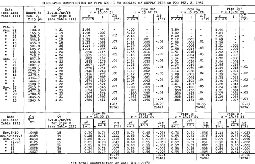
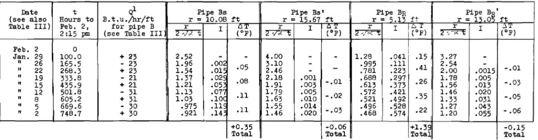
SEASON

The calculations involved in determining the pipe surface temperatures at any time during the heating season,

although not difficult, were very extensive. Consequently

the data used in determining only one temperature (supply pipe Cs for 2:15 p.m. February 2, 1951), will be given here as an example.

Calculations (Tables Al, A2, A3,) involved only

the methods of (1) and use of the line-source

relation-ship, equation 2 1

6.T =

--9.-

I ( r ) (2)

2/(k ＲｾＭＧ

with appropriate substitutions for Ql, r, and t. (k was

taken as 1.0 B.t.u./hr/ft/oF ｡ｮ､ｾ as 0.04 ft 2/hr.) The

contribution of each pipe to the cooling of pipe Cs was calculated from equation 2 using the distance betvleen the pipe in question and Cs (Fig. 12), and the difference between the time when any particular period of operation began or ended and the final time, (Feb.2, 2:15 p.m.).

The value of the function I was first calculated, then the

difference ｢･ｴｷ･･ｾ I for the beginning and end of the

operating period was multiplied by the appropriate value Ql

of Ｒｾｫ to obtain the net contribution to temperature

decrease.

ground the For the virtual or imaginary pipes above thevalues of ｾ were the negatives of those in 21fk

the corresponding real pipes, hence their temperature "decrease" contributions were negative.

For times greater than 2000 hours the derivative of equation 2, with respect to time was used to obtain

better computation accuracy. Since the operating periods

of the heat pump were small compared to 2000 hours the differential form of the derivative could be used, i.e.,

D. (6T) =

Ｔｾｫ

Ｈｌ｜ｾＩ

e

Where: 6. (b..T) is the contribution to temperature "decrease"

caused by heat extraction at rate

Q1

for time period 6t;

and tm is the mean time from the period in question to

the final time. (Note: in Table A, 6. (6. T) is written

The total contributions of all pipes to the cooling of pipe Os (Table A), were as follows:

Pipe 0

Pipe D Pipe B Pipe E Total

In the calculations it was necessary to have high

precision due to the additive effect of the temperature

reduction elements. The final total was rounded off to

two figures, however, since the factor Ql had no greater precision.

The calculated temperature at Os was determined by sUbtractint; the total temperature "decrease" from the

normal ground temperature at the pipe depth. This normal

temperature was taken as the average of the measured temperatures 6 ft beyond the outermost pipes A and E,

(Fig. 1). A small correction of 1.10F (calculated by

the methods above), was added to the normal temperature beyond pipe E to account for the cooling due to the pipe. No correction was necessary for the normal temperature

beyond pipe A since this pipe had not been in use. The

two corrected normal temperatures were 40.5° and 41.4°F,