Cooperation and competition : modeling intention and behavior in dual-agent interactions

Cooperation and Competition: Modeling Intention

and Behavior in Dual-Agent Interactions

by

Lily Zhang

S.B., Massachusetts Institute of Technology (2017)

Submitted to the Department of Electrical Engineering and Computer

Science

in partial fulfillment of the requirements for the degree of

Master of Engineering in Electrical Engineering and Computer Science

at the

MASSACHUSETTS INSTITUTE OF TECHNOLOGY

June 2018

c

○ Massachusetts Institute of Technology 2018. All rights reserved.

Author . . . .

Department of Electrical Engineering and Computer Science

May 25, 2018

Certified by . . . .

Joshua B. Tenenbaum

Professor

Thesis Supervisor

Certified by . . . .

Max Kleiman-Weiner

Ph.D.

Thesis Supervisor

Accepted by . . . .

Katrina LaCurts

Chair, Master of Engineering Thesis Committee

Cooperation and Competition: Modeling Intention and

Behavior in Dual-Agent Interactions

by

Lily Zhang

Submitted to the Department of Electrical Engineering and Computer Science on May 25, 2018, in partial fulfillment of the

requirements for the degree of

Master of Engineering in Electrical Engineering and Computer Science

Abstract

A major goal of artificial intelligence research today is to build something that can cooperate with humans in an intelligent manner. In order to do so, we first must un-derstand the mental mechanisms human use when solving problems of cooperation in dual-agent interactions, or between two people. We used reinforcement learning and Bayesian modeling to create a mathematical representation of this mental model. Our model is comprised of a high-level planner that understands abstract social intentions, and it employs two low-level planners that perform cooperative and competitive plan-ning. To validate the model, we ran two experiments via Amazon Mechanical Turk to capture how humans attribute other players’ behaviors and how they themselves behave in problems of cooperation such as the prisoner’s dilemma. We compared our model against lesioned models and found that our model, which used both cooper-ative and competitive planning strategies, was the most representcooper-ative of the data collected from both experiments.

Thesis Supervisor: Joshua B. Tenenbaum Title: Professor

Thesis Supervisor: Max Kleiman-Weiner Title: Ph.D.

Acknowledgments

Thank you to Dr. Max Kleiman-Weiner and Professor Josh Tenenbaum for your supervision and support throughout this project. I have learned so much over the past year, and I’ve had a great time working on this project.

Thank you to my mom, dad, and brother for always being there for me to lean on not just this year, but throughout my time at MIT. I couldn’t have done this without you guys!

Thank you to all my friends who have kept me going, especially during these last few weeks of thesis-writing. Every single hug, snack, and word of encouragement has meant the world to me.

Contents

1 Background 17

1.1 Introduction . . . 17

1.2 Related Work . . . 18

1.2.1 Social Dilemma . . . 18

1.2.2 Iterated Prisoner’s Dilemma . . . 19

1.2.3 Stochastic Grid Games . . . 21

1.2.4 Social Goal Inference and Attribution . . . 21

2 Stochastic Grid Games 23 2.1 Game Rules . . . 23

2.2 Types of Games . . . 24

2.2.1 Prisoner’s Dilemma Game . . . 24

2.2.2 Four-Way Game . . . 25

2.2.3 Double Fence Game . . . 28

2.2.4 Prisoner’s Dilemma with Fences . . . 28

2.3 Computational Framework . . . 29 2.3.1 Low-level models . . . 29 2.3.2 High-level models . . . 31 2.3.3 Software Architecture . . . 35 3 Attribution Experiment 37 3.1 Experimental Design . . . 37 3.2 Software Architecture . . . 39

3.3 Results and Analysis . . . 39 3.3.1 Parameter Optimization . . . 40 3.3.2 Model Comparison . . . 46 3.4 Discussion . . . 48 3.5 Future Optimizations . . . 49 4 Two-Player Experiment 51 4.1 Experimental Design . . . 51 4.2 Software Architecture . . . 53 4.2.1 Front End . . . 53 4.2.2 Back End . . . 53 4.2.3 Data Analysis . . . 54

4.3 Results and Analysis . . . 55

4.3.1 Parameter Optimization . . . 56

4.3.2 Metrics of Comparison . . . 56

4.3.3 Model Comparison . . . 61

4.4 Discussion . . . 62

4.5 Future Optimizations . . . 63

5 Conclusion and Future Work 65

A Attribution Experiment Data 69

List of Figures

1-1 A prisoner’s dilemma payoff matrix. The Nash equilibrium strategy is to betray because the expected value of staying silent is 0.5(−1) + 0.5(−3) = −2, whereas the expected value of betraying is 0.5(0) + 0.5(−2) = −1. . . 19

2-1 A classic prisoner’s dilemma game. The payoff matrix based on the game rules in Section 2.1 shows the expected reward of each player depending on if the players are cooperative or competitive. If both players were to go for the outer goals, they would each lose 3 points (1 point per turn) and earn 10 points, receiving 10 - 3 = 7 points overall. If they were to both go for their closer goal, they would collide in the center square, and only one player would make it to their goal. Because each player has an equally likely chance of reaching their goal first, the expected reward is 0.5(10) + 0.5(0) = 5, giving a net 5 - 3 = 2 points (3 points were lost total, 1 for each of 2 turns and and 1 for the collision). Finally, if one player went for the inner goal while the other went for the outer goal, the competing player would receive 10 - 2 = 8 points, while the cooperating player would receive 0 - 2 = -2 points. In prisoner’s dilemma fashion, the expected value of competing (0.5(2) + 0.5(8) = 5) is higher than that of cooperating (0.5(7) + 0.5(-2) = 2.5). 26

2-2 The four way game, which is another social dilemma game. If both players cooperate, they each take 5 turns and both receive the 10 point reward, ending with net 10 - 5 = 5 points each. If one player competes while the other cooperates, it takes the competing player only 4 turns to reach the 10 points reward, ending with net 10 - 4 = 6 points. However, the cooperating player does not reach their goal, so they end with 0 - 4 = -4 points. In the case that both players compete, each player has a 50% chance of reaching their goal in 4 turns (which incurs 5 points because of the extra point lost from colliding in the center square), ending with an expected point value of 0.5(10) + 0.5(0) - 5 = 0. Again, the expected value of competing (0.5(6) + 0.5(0) = 3) is higher than that of cooperating (0.5(5) + 0.5(-4) = 0.5). . . 27

2-3 A game using fences (denoted by the red dotted lines), which a player has a 75% chance of crossing successfully. Because players may not be able to make the moves that they intended to, the game may result in a different outcome from what the players were originally intending. The added probability complicates the expected payoff, so the calculation was omitted. . . 28

2-4 The PDF (prisoner’s dilemma with fences) game. It is the original prisoner’s dilemma game from Figure 2-1 but with fences added in front of the goals, combining social dilemma with testing for intention versus outcome. The added probability complicates the expected payoff, so the calculation was omitted. . . 29

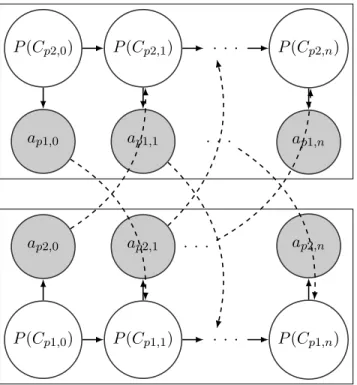
2-5 The HMM graphical model representing the CCAgent’s action obser-vation and belief update in dual-agent interactions. The top nodes represent player 𝑝1, and the bottom nodes represent player 𝑝2. On each step 𝑖 from 0 to 𝑛, each player 𝑝 has a belief 𝑃 (𝐶𝑝_𝑜𝑡ℎ𝑒𝑟,𝑖) of

how cooperative the other player is. Using this belief, they generate a policy 𝜋𝑝 from which they select their next action 𝑎𝑝,𝑖. Then, each

player observes the other player’s 𝑎𝑖 and updates their own belief state

𝐶𝑝_𝑜𝑡ℎ𝑒𝑟,𝑖+1. The shaded nodes represent the observations and the

dot-ted lines represent the belief updates. . . 33

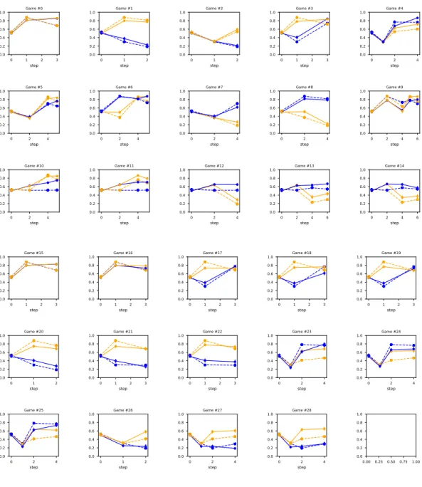
3-1 Plots of each game sequence showing the human (solid) and model (dotted) values (using a single 𝛽 and 𝑑) per judgment point per player. (The yellow player is displayed in orange for better visibility.) Games 0-4 are prisoner’s dilemma games, games 5-9 are four-way games, games 10-14 are double fence games, and games 15-28 are PDF games. . . . 42 3-2 A comparison between the optimized single decay and optimized

asym-metric decays. The dotted line shows the transition from 𝐶0to 𝐶1using

a single decay 𝑑 = 0.159, and the solid line shows the transition us-ing the asymmetric decays 𝑑𝑎 = 0.0867 and 𝑑𝑏 = 0.307. The 𝐶1 for

asymmetric decays is higher, showing that the judgments end up being more cooperative-leaning. . . 44 3-3 Plots of each game sequence showing the human (solid) and model

(dotted) values (using a single 𝛽 and asymmetric 𝑑) per judgment point per player. The fit compared to Figure 3-1 is improved, indicating that these parameters are reflective of the human mental model. . . 45 3-4 A comparison of the human versus model values per judgment point

using a single decay 𝑑 (left) and asymmetric 𝑑s (right). The correlation using a single 𝑑 was 𝑅 = 0.899, 𝑅2 = 0.809, 𝑅𝑀 𝑆𝐸 = 0.107. The

correlation using asymmetric 𝑑s was 𝑅 = 0.938, 𝑅2 = 0.879, 𝑅𝑀 𝑆𝐸 =

3-5 The fit between human and model values per judgment point for the le-sioned models (Cooperate-Random on the left, and Random-Compete on the right). The values are quite scattered, with no strong positive correlation. . . 47

4-1 The relationship between the server and its clients, designed such that minimal information needs to be passed back and forth. When a player makes a move on step 𝑖, the client will send its current state and the selected action to the server. Once the server receives the message from both players, it will calculate the next joint-state and send it back to each client. . . 55

4-2 A plot of each model’s model likelihood as a stacked bar for each par-ticipant, sorted by how representative CCAgent is of that participant. This provides an overview of how the different models captured the human mental model at a granular, per player level. CCAgent is the dominant model, occupying the most area in this graph. . . 59

4-3 Plots of the log data likelihood ln(𝑃 (𝐷|𝑀 )) (left) and the model like-lihood 𝑃 (𝑀 |𝐷) (right) per model. It is evident that the CCAgent is the best fit to the experimental data, especially when comparing the model likelihoods. . . 60

4-4 The average likelihood of selecting the participant’s next action for each model, a metric of "correctness." CCAgent is a hair higher than CompeteAgent, RandomCCAgent, and OutcomeAgent, but that can be attributed to the fact that at certain states in the game, there is only one possible, rational next movement, and that is captured by all four of these models. . . 61

4-5 A closer look at specific model comparisons. The top row shows the log data likelihoods for each model (the colors correspond to Figures 4-2 and 4-4), and the bottom row shows the model likelihoods. From left to right, the comparisons show CCAgent vs the low-level mod-els, CCAgent vs RandomCCAgent, and CCAgent vs OutcomeAgent. It is evident that CCAgent is the best fit to the experimental data, especially when comparing the model likelihoods. . . 62

5-1 A histogram showing the RMSE between each participant’s judgments and the sample mean judgments in the attribution experiment, or their "accuracy of judgment." The distribution is right-skewed, with the highest density between 0.2 and 0.3, showing that there exists a range of accuracy. This could potentially be used to determine if there’s a correlation between how accurately people make judgments and how they play the grid games. . . 67

A-1 This flowchart shows all 5 game sequences for the prisoner’s dilemma game. The sequences from top to bottom correspond to games 0, 3, 1, 4, and 2 from the experiment. . . 70

A-2 This flowchart shows all 5 game sequences for the four-way game. The sequences from top to bottom correspond to games 5, 7, 6, 8, and 9 from the experiment. Game 9 is notable because there is a high degree of miscoordination between the two players before they eventually reach the cooperative outcome. . . 71

A-3 This flowchart shows all 5 game sequences for the double fence game. They correspond to games 10, 11, 12, 13, and 14 from the experiment. 72

A-4 This flowchart shows the first 8 game sequences for the prisoner’s dilemma with fences game, corresponding to games 15-22 from the experiment. Each game sequence from A-1 now has 3 possible out-comes: both players reach the goals, only blue reaches the goal, and only yellow reaches the goal. This resulted in 14 total game sequences (one was removed due to symmetry). . . 73 A-5 This flowchart shows the last 6 game sequences for the prisoner’s

dilemma with fences game, corresponding to games 23-28 from the experiment. . . 74

List of Tables

3.1 A comparison of the optimized values from fitting the CCAgent model with different set of free parameters. Using asymmetric decays had a marked improvement in the fit, but using asymmetric 𝛽s did not. . . 46 3.2 A comparison of the optimized values using the CCAgent,

Cooperate-Random Agent, and Cooperate-Random-Compete Agent and how well each model fit to the experimental data. Clearly, the CCAgent outperformed both lesioned models. . . 48 4.1 A table showing which free parameters each model depended on. . . . 56 4.2 A comparison between using different sets of free parameters. As in

Section 3.3.1, a single 𝛽 and asymmetric decays was found to improve the fit and also run within a reasonable amount of time. . . 56 4.3 The optimized parameters for each model. Both CoopAgent and

Com-peteAgent have very low 𝛽s, which mean they are quite noisy models. In comparison, the high-level agents have higher 𝛽s, indicating they are able to fit to the two player data without needing to introduce much noise. . . 57

Chapter 1

Background

1.1

Introduction

Cooperation is a tricky and ambiguous problem that humans face every single day, from determining if others are being cooperative, to deciding whether or not to behave cooperatively. Say you’re taking a class where only the top 10% of students get A’s. Do you cooperate with your classmates and study together in an effort to all get A’s? Do you instead compete and study alone to increase your own chances of getting the A? Your classmate asks you to take a break with them - is this a friendly gesture to help you destress? Or are they trying to get you to study less and fail? Sometimes people intend to cooperate, but due to some miscoordination, the outcome ends up going the other way. Let’s say your friend lent you their flashcards, but it ended up being the wrong material, causing you to do poorly in the class. Did your friend make a well-intentioned mistake? Or did they have some ulterior motive?

As you can see, cooperation can be hard to determine, especially when the data is sparse and noisy. However, humans as young as pre-verbal infants are able to do this seemingly common sense attribution on a daily basis [7]. If we want to build machines that can work with humans, we must first understand how cooperative decision making processes in the mind work, and how we as humans attribute and respond to cooperative and competitive behavior in dual-agent interactions between two people. By building a mathematical model of this type of human cooperation, we

can gain insight on the mechanisms at play when humans try to cooperate with each other, a vital facet of life encompassing everything from sharing on the playground to international diplomacy. From a computer science standpoint, we can eventually use these ideas to create artificial intelligence that can interact and cooperate with humans in a human-like and intelligent manner. This is especially important in this day and age given the rapid ubiquity of "smart" technology everywhere, from our phones, to our cars, to our homes.

This thesis consists of five total chapters. Chapter one provides an introduction to and related work about the problem at hand. Chapter two discusses the stochastic grid games and computational framework used to model this problem. Chapter three describes the first of two experiments, the attribution experiment. In this experiment, we explored how humans attribute cooperative and competitive behavior to players playing stochastic grid games. Chapter four discusses the second experiment, the two player experiment where human participants played the stochastic grid games against each other. This allowed us to evaluate how humans actually played these games and how to best model the way they played the game. Finally, chapter five provides a summary of the experiments and findings and also outlines future work to be done in this area.

1.2

Related Work

There has been much research surrounding evolutionary and game theoretic studies on cooperation and how humans behave in these situations.

1.2.1

Social Dilemma

A heavily studied cooperation problem is social dilemmas, or situations with a conflict between personal and collective interest. Maximizing one’s own personal interest is advantageous if everyone else continues to maximize the collective interest. However, if everyone chooses to maximize their own personal interest, everyone would be worse off than if everyone chose to maximize the collective interest. The dilemma presents

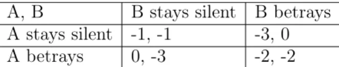
A, B B stays silent B betrays A stays silent -1, -1 -3, 0 A betrays 0, -3 -2, -2

Figure 1-1: A prisoner’s dilemma payoff matrix. The Nash equilibrium strategy is to betray because the expected value of staying silent is 0.5(−1) + 0.5(−3) = −2, whereas the expected value of betraying is 0.5(0) + 0.5(−2) = −1.

itself when, in a single instance, maximizing one’s own personal interest is actually the dominant strategy. This is because the expected value from being selfish is higher than the expected value from maximizing the collective interest, despite the fact that total collective interest in the population is better than total personal interest.

Figure 1-1 shows an example of a prisoner’s dilemma problem [13], one of the most widely studied social dilemmas. In the prisoner’s dilemma, two prisoners’ decisions on how to act determine the lengths of their prison sentences, where "stays silent" is the collective interest and "betrays" is the personal interest. Assuming that the other person is equally likely to stay silent or betray, the expected value from betraying is higher (a lower prison sentence) than from staying silent. Thus, betrayal is the dominant strategy. So how is it that cooperation is able to manifest in a selfish population?

1.2.2

Iterated Prisoner’s Dilemma

An interesting case arises with iterated prisoner’s dilemma, which was studied ex-tensively by Robert Axelrod in his book The Evolution of Cooperation [1]. Iterated prisoner’s dilemma is when prisoner’s dilemma is conducted for multiple rounds with memory of the previous rounds. Previously, in a single round, there was no penalty for mutual defection. However, with repeated rounds, the players now have an ongoing relationship that requires more strategic reasoning, and defection is not necessarily the dominant strategy anymore.

Axelrod hosted a tournament to study the best-performing strategy when play-ing iterated prisoner’s dilemma. There were four main distplay-inguishplay-ing properties of

strategies that performed well. The most important property was being "nice," which meant not being the first to defect. The top 8 entries were all "nice" strategies, and the rest were all not "nice." However, it was also important not to be overly nice or overly mean - when the other player defects, it’s important to retaliate, but when the other player returned to cooperation, it’s also important to forgive. The final property was to not be envious, which meant not trying to score more points than the other player.

A strategy called tit for tat (TFT), submitted by Anatol Rapoport [14], won the tournament despite being the simplest algorithm. TFT started in the cooperative mode, and on subsequent rounds it switched to whichever mode the other player used on the previous round. TFT was also able to perform well with itself and generally avoid being exploited, indicating that this type of reciprocity is an important social norm.

Nowalk and Sigmund [12] introduced a new strategy called Pavlov, or "win-stay, lose-shift." If a player won a round, they would stay with the same strategy, and if they lost a round, they would shift to the opposite strategy. "Win-stay lose-shift" echoes a Pavlovian effect of responding positively to a reward and negatively otherwise, which is behavior found in many animals [5].

Pavlov is superior to TFT in its ability to account for noise and correct for mis-takes. When two TFT players play against each other, if one makes a mistake and accidentally defects, the two will be stuck in a cycle of switching between defection and cooperation indefinitely. However, two Pavlov players will mutually defect for only one round before switching back to mutual cooperation. In a study of mutual-selection dynamics with error, Pavlov was selected as the dominant model if the benefit of cooperation exceeded a certain threshold, but TFT was never dominant [9]. An iteration of TFT called "generous tit for tat" can account for mistakes by employing a fixed probability of switching to the cooperative strategy, but it is still not as efficient as Pavlov [12]. Being able to account for noise is important as co-operation in the real world is quite susceptible to errors, and a high likelihood of miscoordination could greatly disrupt equilibrium strategies [2].

1.2.3

Stochastic Grid Games

De Cote and Littman studied problems of cooperation and dominant strategies by using stochastic two-player grid games. These games, which our research builds upon, are defined by ⟨𝑆, 𝑠0, 𝐴1, 𝐴2, 𝑇, 𝑈1, 𝑈2⟩. 𝑆 is the set of all possible states, with a

starting state of 𝑠0 where 𝑠0 ∈ 𝑆. Each agent has a set of actions, 𝐴1 and 𝐴2

respectively, forming the joint action space 𝐴1 × 𝐴2. For each joint state and joint

action pair (𝑠, 𝑎1, 𝑎2), the one step state-transition function is defined as 𝑇 (𝑠, 𝑎1, 𝑎2) =

𝑃 (𝑠′|𝑠, 𝑎1, 𝑎2), which gives the probability of choosing a new state 𝑠′ ∈ 𝑆 given the

current joint state and joint action. The transition functions of each joint state and joint action pair all together make up a policy 𝜋(𝑎|𝑠). Each agent tries to maximize its own utility 𝑈 , which is a function of 𝑠′, 𝑠, 𝑎1, 𝑎2, and the policy that encodes

the maximum expected utility is the optimal policy. Using these games, de Cote and Littman were able to build an algorithm that could find fair Nash equilibrium solutions in repeated rounds [3].

Expanding on de Cote and Littman’s work with stochastic grid games, Max Kleiman-Weiner et al. developed a hierarchical model of social planning to model how humans would behave in repeated rounds of different two-player games. The full model that coordinated low-level action plans and high-level strategic goals was the best at capturing the rates of cooperation from the behavioral experiment, indicating that it mostly closely reflected the hierarchical model of social planning that humans use to cooperate and compete [10]

These social dilemma games and strategies mirror real-life paradigms when it comes to cooperation and competition, and they provide a basis for how our model can infer these different behaviors and respond appropriately.

1.2.4

Social Goal Inference and Attribution

Though it’s important to study how people behave in problems of cooperation, it is equally important to understand is how people infer and attribute cooperative behavior, especially under suboptimal conditions. Remarkably enough, humans are

able to create rich inferences from stimuli as simple as shapes moving in a 2D plane [8].

One type of social goal attribution was formalized by Tomer Ullman et al. by de-veloping a model that could infer if one agent was helping or hindering the other, with no knowledge of either agent’s goal. The model was also able to perform judgments from relatively few observations. The model was able to capture some of the complex-ity of the human mental model, providing a far better fit than a simple perceptual cue-based model [16].

People can also attribute levels of intelligence based off of viewing a series of actions. In a study by Marta Kryven et al., people attributed intelligence to one of two main types of planners: those who used some sort of a strategy, and those who reached a positive outcome [11]. This illuminated the idea that there can be multiple ways to attribute intelligence, whether that was based on if the agent behaved in a human-like way or was able to reach the goal in fewer steps.

This introduced another interesting dichotomy of being clever versus being lucky. Gerstenberg et al. explored how people assigned credit when something unexpected happened, whether it was due to that person’s skill and intellect or if it was a fluke [6]. He found that both the expectations and the context played a major role in how people placed responsibility upon others.

Though our study will focus specifically on attributing and inferring cooperative and competitive behavior, these different branches of attribution are important to keep in mind for exploration and possible future directions our model could expand.

Chapter 2

Stochastic Grid Games

To study this problem of modeling cooperative and competitive intention and behav-ior, we used two-player stochastic grid games as our environment based off of the same formalization as de Cote and Littman’s work [3] referenced in Section 1.2.3. We assumed that each player operated under the principle of rationality [4], which states that the agents will take the most efficient actions to reach their respective goals. These games include and build upon ones originally used in Kleiman-Weiner’s study on repeated stochastic games [10].

2.1

Game Rules

Each player is represented by either a blue circle or a yellow circle, and they have a goal of their own color worth 10 points that they are trying to reach. Each grid is configured such that there can be multiple ways for each player to reach their goal, and players can also have more than one goal of their own color. Players are also able to enter each other’s goals to no effect. An example of a game can be seen in Figure 2-1.

Players are allowed to move one square up, down, left, right, or stay in place. Players lose 1 point per turn they take, even if they just wait in place. The game updates simultaneously, which means that both players must choose their next move before the moves are made and the game state is updated.

The game ends when at least one player reaches their goal. For both players to receive the 10 point reward, they must enter their respective goals on the same turn, which is the cooperative outcome. Otherwise, only one player will receive the 10 point reward, which is the competitive outcome in favor of whoever reached the goal first. The game will always end in either a cooperative or competitive outcome.

There are also illegal movements. Because the two players have no way of com-municating beyond what movements they are making, collisions are possible. All collisions cost 1 extra point for the player(s) that initiated the collision. There are three types of collisions. Only one player can occupy a square at a time. When two players try to move into the same square, a coin flip will determine which player is successful (which means both players have an equal chance of "winning" and suc-cessfully making it into the target square), and both players lose an extra point. If players try to swap spots, they will be bounced back to their previous square, and both players will lose an extra point. Finally, a player cannot enter a square that another player occupies. If a player tries to move into the square of a stationary player, that player will lose an extra point.

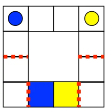
Another feature of the games is fences, which are denoted by red dotted lines, as seen in Figure 2-3. Fences are barriers in between spaces, and if a player tries to move across a fence, they only have a 75% chance of successfully doing so.

2.2

Types of Games

The following describes the types of games that were used in the experiments to test for cooperative and competitive intention and behavior.

2.2.1

Prisoner’s Dilemma Game

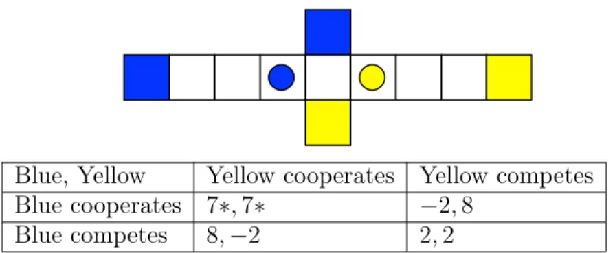
We can structure the grid game to be like a prisoner’s dilemma [3, 10], as seen in Figure 2-1. In this game, each player has two goals. Reaching the outer goals takes 3 steps, whereas reaching the inner goals takes 2 steps. If a player were playing alone, it makes sense to take the shortest path in order to maximize their score. However,

the introduction of another player makes things more complicated, which is reflected in the payoff matrix shown in Figure 2-1. Each player could behave cooperatively and try to reach the goals at the same time, or they could behave competitively and try to reach their own goal first. As seen, the expected value of competing and trying to maximize one’s own score is higher than that of cooperating.

It may seem like the only cooperative route is for both players to go for the outer goals, and the only competitive route is for both to go for the inner goals. However, there are more possibilities - for example, one player could first choose to go for the inner goal and then wait for the other player, which would also lead to a cooperative outcome despite one player ending in the inner goal. It is also possible to make mistakes on this grid. For example, two players intending to cooperate could both choose to move into the center square on their first turn and collide on accident. The player who moved into the intersection successfully could wait a turn after the intersection for the other player to move closer to their goal, ultimately resulting in a cooperative outcome. This type of interaction demonstrates that miscoordination can be an attribute of cooperation and does not necessarily detract from it.

2.2.2

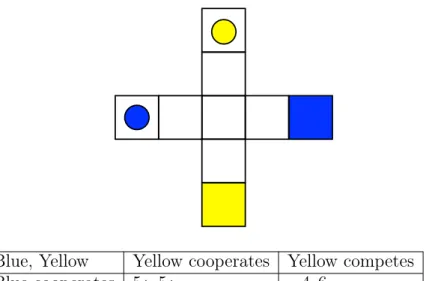
Four-Way Game

Another example of a social dilemma is the four-way game, shown in Figure 2-2. In this game, each player’s goal is located opposite a four-way intersection. Because only one player can occupy a square at a time, the cooperative outcome is only possible if a player waits for the other player to catch up before proceeding to their own goal. Otherwise, whichever player occupies the intersection square first will reach the goal first, resulting in the competitive outcome. Because there is an equal chance of each player ending up in the intersection square first, there competitive outcome is equally likely to be in the favor of either player.

As seen in the matrix in Figure 2-2, the payoff structure for the four-way game follows that of a social dilemma as well (assuming no unintended collisions). As with the prisoner’s dilemma game, this game also allows for mistakes of coordination when deciding which player should move into the intersection square first.

Blue, Yellow Yellow cooperates Yellow competes Blue cooperates 7*, 7* −2, 8

Blue competes 8, −2 2, 2

*assuming no miscoordination

Figure 2-1: A classic prisoner’s dilemma game. The payoff matrix based on the game rules in Section 2.1 shows the expected reward of each player depending on if the players are cooperative or competitive. If both players were to go for the outer goals, they would each lose 3 points (1 point per turn) and earn 10 points, receiving 10 - 3 = 7 points overall. If they were to both go for their closer goal, they would collide in the center square, and only one player would make it to their goal. Because each player has an equally likely chance of reaching their goal first, the expected reward is 0.5(10) + 0.5(0) = 5, giving a net 5 - 3 = 2 points (3 points were lost total, 1 for each of 2 turns and and 1 for the collision). Finally, if one player went for the inner goal while the other went for the outer goal, the competing player would receive 10 - 2 = 8 points, while the cooperating player would receive 0 - 2 = -2 points. In prisoner’s dilemma fashion, the expected value of competing (0.5(2) + 0.5(8) = 5) is higher than that of cooperating (0.5(7) + 0.5(-2) = 2.5).

Blue, Yellow Yellow cooperates Yellow competes Blue cooperates 5*, 5* −4, 6

Blue competes 6, −4 0, 0

*assuming no miscoordination

Figure 2-2: The four way game, which is another social dilemma game. If both players cooperate, they each take 5 turns and both receive the 10 point reward, ending with net 10 - 5 = 5 points each. If one player competes while the other cooperates, it takes the competing player only 4 turns to reach the 10 points reward, ending with net 10 - 4 = 6 points. However, the cooperating player does not reach their goal, so they end with 0 - 4 = -4 points. In the case that both players compete, each player has a 50% chance of reaching their goal in 4 turns (which incurs 5 points because of the extra point lost from colliding in the center square), ending with an expected point value of 0.5(10) + 0.5(0) - 5 = 0. Again, the expected value of competing (0.5(6) + 0.5(0) = 3) is higher than that of cooperating (0.5(5) + 0.5(-4) = 0.5).

Figure 2-3: A game using fences (denoted by the red dotted lines), which a player has a 75% chance of crossing successfully. Because players may not be able to make the moves that they intended to, the game may result in a different outcome from what the players were originally intending. The added probability complicates the expected payoff, so the calculation was omitted.

2.2.3

Double Fence Game

In the game shown in Figure 2-3, there are two sets of fences. The players start the same distance away from the first fence and both try to cross their respective fence. If only one player gets over the first set of fences, they could demonstrate cooperative intent by waiting for the other player to cross successfully before continuing towards their goal. In addition, there are a second set of fences in front of the goals. The two players could try to move into their own goals at the same time, but one player could cross the fence successfully while the other does not, resulting in what looks like a competitive outcome despite the intended cooperation. The fences could also hold up a competitive player, causing them to ultimately reach their goal at the same time as the other player, a cooperative outcome contrary to the competitive intent. By using these fences, we can demonstrate that understanding cooperative intent requires more than just examining the final outcome of the players - it’s necessary to infer the entire sequence of movements made by both players.

2.2.4

Prisoner’s Dilemma with Fences

To capture both concepts of social dilemma and intention versus outcome, we created the prisoner’s dilemma with fences game (PDF) shown in Figure 2-4. PDF is the

original prisoner’s dilemma game shown in Figure 2-1 but with a fence added in front of each goal. The original structure of the grid provides the social dilemma aspect, and because the fences can block movements, the final outcome may not reflect the original intention.

Figure 2-4: The PDF (prisoner’s dilemma with fences) game. It is the original pris-oner’s dilemma game from Figure 2-1 but with fences added in front of the goals, combining social dilemma with testing for intention versus outcome. The added probability complicates the expected payoff, so the calculation was omitted.

2.3

Computational Framework

In our model, an extension of Kleiman-Weiner’s hierarchical planner [10], each player is represented by a high-level planning agent that can infer abstract social goals and employs two separate low-level types of policy generation, a cooperative planner and a competitive planner. We believe that this high-level planner composed of both cooperative and competitive elements is more representative of the mental model humans use in these problems of cooperation than a planner that uses a single policy.

2.3.1

Low-level models

The low level models generate policies 𝜋(𝑎|𝑠) that define the likelihood of taking actions 𝑎 given state 𝑠. The policies differ based on the overall abstract goal - either cooperative or competitive.

2.3.1.1 CoopAgent

The cooperative planner, or CoopAgent, uses value iteration [15] over the joint action space (defined in Equations 2.1 and 2.2) to compute an optimal MDP policy and its value for the joint agent based on all the possible joint states and actions in a given game. The joint agent can be thought of as a puppetmaster that controls both players in the game, which means that the players will always behave cooperatively. The joint policy is then marginalized over each individual player in order to get each player’s individual cooperative policy. The parameter 𝛽 is used to compute the softmax that determines how noisy the transition probabilities are. In the extreme cases, if 𝛽 = inf, the likelihood 𝑃 (𝑎1, 𝑎2|𝑠) of the joint action (𝑎1, 𝑎2) with the highest likelihood will

equal 1 and the other joint actions will have likelihoods of 0. If 𝛽 = 0, all joint actions will have uniform likelihoods.

𝑃 (𝑎1, 𝑎2|𝑠) = 𝜋𝐺(𝑠, 𝑎1, 𝑎2) ∝ 𝑒(𝛽𝑄 𝐺_(𝑠,𝑎 1,𝑎2)) _(2.1) 𝑄𝐺(𝑠, 𝑎1, 𝑎2) = Σ𝑠′𝑃 (𝑠′|𝑠, 𝑎₁, 𝑎₂)[𝑈𝐺(𝑠′, 𝑠, 𝑎₁, 𝑎₂)+ (2.2) max (𝑎′₁,𝑎′₂)𝑄 𝐺 (𝑠′, 𝑎′₁, 𝑎′₂)] 2.3.1.2 CompeteAgent

The competitive planner, or CompeteAgent, calculates its policy recursively for 𝑘 levels. It starts with one of five predefined level-0 models of the other player: 1) static, where the other player doesn’t move, 2) solo, where the other player is playing as if it’s alone; 3) friend, where the other player moves out of the way; 4) cooperative, where the other player behaves cooperatively, and 5) random, where the other player moves randomly. In our model, we use the level-0 solo model with 𝑘 = 1. The 𝛽 parameter used in cooperative policy generation is also used here. The level-0 model

for the other player is defined as: 𝑃 (𝑎𝑖|𝑠, 𝑘 = 0) = 𝜋𝑖0(𝑠) ∝ 𝑒(𝛽𝑄 0 𝑖(𝑠,𝑎𝑖) _(2.3) 𝑄0_𝑖(𝑠, 𝑎𝑖) = Σ𝑠′𝑃 (𝑠′|𝑠, 𝑎_𝑖)[𝑈_𝑖(𝑠, 𝑠, 𝑎_𝑖, 𝑠′) + max (𝑎′ 𝑖) 𝑄0_𝑖(𝑠′, 𝑎′_𝑖)] (2.4)

The CompeteAgent then calculates its policy by best-responding to the level-0 model and maximizing its own reward, and it can do so recursively for 𝑘 levels using the following equations:

𝑃 (𝑎𝑖|𝑠, 𝑘) = 𝜋𝑖𝑘(𝑠) ∝ 𝑒 (𝛽𝑄𝑘 𝑖(𝑠,𝑎𝑖) _(2.5) 𝑄𝑘_𝑖(𝑠, 𝑎𝑖) = Σ𝑠′𝑃 (𝑠′|𝑠, 𝑎_𝑖)[𝑈_𝑖(𝑠, 𝑠, 𝑎_𝑖, 𝑠′) + max (𝑎′_𝑖) 𝑄 𝑘 𝑖(𝑠 ′ , 𝑎′_𝑖)] (2.6) 2.3.1.3 RandomAgent

To provide a point of comparison for the Coop- and CompeteAgents, we created a lesioned model, the RandomAgent which does no planning at all. There is a uniform distribution over all valid actions, which means 𝑃 (𝑎 = 𝑎𝑖|𝑠) = _𝑁1 for all valid actions

𝑎𝑖, where 𝑁 is the total number of next actions.

2.3.2

High-level models

When playing the game, the high-level agent observes the other player’s action and infers abstract social goals of cooperation and competition. Based on its inference, it then uses the low-level planners to generate a policy to select the next action. This Hidden Markov Model (HMM) can be seen in Figure 2-5. We have three high-level models, the CCAgent, the RandomCCAgent, and the OutcomeAgent (the latter two are lesioned models used for comparison).

2.3.2.1 CCAgent

Our primary high-level agent is the Cooperate-Compete Agent, or CCAgent for short. We believe that the CCAgent is the most representative of the mental model humans

use when playing these grid games and making inferences about cooperation and competition.

The CCAgent starts with a prior of 0.5, which means that initially it has no knowledge of how cooperative or competitive the other player is, and both policies (cooperative and competitive) are weighted equally. On each step 𝑖, the agent ob-serves the other player’s action 𝑎2. Then using the policies for both the cooperative

and competitive planners, it determines the relative likelihood of the player being in that state given if it’s cooperative 𝐶 or competitive 𝐶′, denoted by 𝑃 (𝑠, 𝑎1, 𝑎2|𝐶𝑖) and

𝑃 (𝑠, 𝑎1, 𝑎2|𝐶𝑖′), respectively. It then calculates a new posterior probability 𝑃 (𝐶𝑖+1|𝑠, 𝑎1, 𝑎2)

and 𝑃 (𝐶_𝑖+1′ |𝑠, 𝑎1, 𝑎2) of the player. The calculation is also parameterized by decay

𝑑. The decay parameter "decays" the posterior probability to a less extreme value, pulling down higher values and raising up lower values. As decay approaches 0 from the left, the agent is more likely to remain in the same mode as its prior. As decay approaches 1 from the right, the agent is more likely to switch between low-level modes. This is formalized in the following equations:

𝑇 = ⎡ ⎣ 1 − 𝑑 𝑑 𝑑 1 − 𝑑 ⎤ ⎦ ⎡ ⎣ 𝑃 (𝐶𝑖) 𝑃 (𝐶_𝑖′) ⎤ ⎦ (2.7) 𝑃 (𝐶𝑖+1|𝑠, 𝑎1, 𝑎2) ∝ 𝑃 (𝑠, 𝑎1, 𝑎2|𝐶𝑖) × 𝑇1 (2.8) 𝑃 (𝐶_𝑖+1′ |𝑠, 𝑎1, 𝑎2) ∝ 𝑃 (𝑠, 𝑎1, 𝑎2|𝐶𝑖′) × 𝑇2 (2.9)

The action observation and belief update can be represented by a Hidden Markov Model, as shown in Figure 2-5. Because the low-level planners provide a layer of abstraction, the high-level planner can use them without considering the details.

The posterior probability 𝑃 (𝐶𝑖+1) = 𝑃 (𝐶𝑖+1|𝑠, 𝑎1, 𝑎2) is the model’s beliefs of

the cooperativeness of the other player after observation and what the agent uses to select its next policy. To create a generous model that always has some probability of switching, we bound 𝑃 (𝐶𝑖+1) by [𝑏, 1 − 𝑏] where 0 ≤ 𝑏 ≤ 0.5. It then uses 𝑃 (𝐶𝑖+1), 𝑏,

𝑃 (𝐶𝑝2,0) 𝑃 (𝐶𝑝2,1) . . . 𝑃 (𝐶𝑝2,𝑛)

𝑎𝑝1,0 𝑎𝑝1,1 . . . 𝑎𝑝1,𝑛

𝑃 (𝐶𝑝1,0) 𝑃 (𝐶𝑝1,1) . . . 𝑃 (𝐶𝑝1,𝑛)

𝑎𝑝2,0 𝑎𝑝2,1 . . . 𝑎𝑝2,𝑛

Figure 2-5: The HMM graphical model representing the CCAgent’s action observation and belief update in dual-agent interactions. The top nodes represent player 𝑝1, and the bottom nodes represent player 𝑝2. On each step 𝑖 from 0 to 𝑛, each player 𝑝 has a belief 𝑃 (𝐶𝑝_𝑜𝑡ℎ𝑒𝑟,𝑖) of how cooperative the other player is. Using this belief,

they generate a policy 𝜋𝑝 from which they select their next action 𝑎𝑝,𝑖. Then, each

player observes the other player’s 𝑎𝑖 and updates their own belief state 𝐶𝑝_𝑜𝑡ℎ𝑒𝑟,𝑖+1.

The shaded nodes represent the observations and the dotted lines represent the belief updates.

where:

𝜋𝑤𝑒𝑖𝑔ℎ𝑡𝑒𝑑 = (𝑃 (𝐶𝑖+1)((1 − 2𝑏) + 𝑏)𝜋𝑐𝑜𝑜𝑝𝑒𝑟𝑎𝑡𝑒+ (𝑃 (𝐶𝑖+1′ )((1 − 2𝑏) + 𝑏)𝜋𝑐𝑜𝑚𝑝𝑒𝑡𝑒 (2.10)

This weighing of policies means that the CCAgent follows a generous tit for tat mentality [12] where it will more likely respond with whatever it observes the other agent did on the previous step, with some probability of switching to the opposite. Essentially, if the other agent is observed to be more cooperative, the agent will weigh the cooperative policy more heavily. Inversely, if the other agent is observed to be more competitive, the agent will weight the competitive policy more heavily, acting reciprocally.

2.3.2.2 RandomCCAgent

We built the RandomCCAgent in order to have a benchmark to demonstrate that observing and updating the belief state about the other agent is necessary. This agent never updates its belief about the other agent’s level of cooperation, which means that the cooperative and competitive policies are always equally weighted. In other words, for each step, the RandomCCAgent is equally likely to use the cooperative and competitive policy to generate its next action regardless of what the other agent is doing.

2.3.2.3 OutcomeAgent

Another important aspect of the CCAgent is that it makes observations after each action and is constantly updating its belief state of the other agent’s level of coop-eration. To validate this aspect of the CCAgent, we built the OutcomeAgent, which only observes the final state of the previous round and then updates its strategy based on the win-stay lose-shift learning strategy described in Section 1.2.2. The OutcomeAgent starts believing the other agent is cooperative, with 𝑃 (𝐶0) = 1. After

each round, if an agent makes it into its own goal, it sees that it has "won" and continues using its current strategy. Otherwise, the agent sees that it has "lost" and

shifts to the opposite strategy. Despite being a lesioned model, we do expect the OutcomeAgent to capture some portion of the population as it employs a learning strategy that is found in nature [5].

2.3.3

Software Architecture

There were three main classes that were used to build out the computational frame-work, and everything was coded in Python. There was a Game object that encoded the properties and rules of the game, as described in Section 2.1. Each new game configuration from Section 2.2 was a subclass of the Game class. There was also an Agent object that represented each of the different low-level and high-level models in Sections 2.3.1 and 2.3.2, and these agents would be the "players" and "observers" of the game. These agents were built using the planning and policy generation code orig-inal written by Kleiman-Weiner [10]. Forig-inally, there was a World class that encoded the interactions between the game and the agents.

Chapter 3

Attribution Experiment

The attribution experiment tested how humans assign cooperative and competitive intent to players playing the grid games, and it served to validate how accurately our model’s observed beliefs reflected those of humans. Two rounds of the attribution experiment were run on Amazon Mechanical Turk (MTurk) with different sets of games. There were 52 and 51 participants, respectively.

3.1

Experimental Design

After consenting to the terms and conditions of our experiment, the participant was shown a series of tutorial slides that instructed the user of the game rules described in Section 2.1. Each slide had a short animation demonstrating an aspect of the game, and participants were able to play the animations as many times as they wanted. See https://youtu.be/_1tSl6GUXsY for a video of the attribution experiment tutorial.

After completing the tutorial, the participant began the experiment. In the exper-iment, the participant watched full game sequences between people playing different grid games (a game sequence here refers to an entire game from the starting state to the final state of one or both players reaching the goal(s)). At various points throughout each game sequence, the game paused, and the participant was asked to evaluate how cooperative each player’s behavior seemed on a sliding scale from "Not Cooperative" to "Cooperative." Participants were not able to evaluate the players

until the current step of the sequence finished playing. Participants were also able to replay the entire game sequence up to the paused point if they needed to.

The first round of the experiment consisted of 15 total different game sequences across 3 games, the prisoner’s dilemma game, the four-way game, and the double fence game (shown in Figures 2-1, 2-2, and 2-3). For each game, there were 5 predefined series of movements per game, which can be seen in Figures A-1, A-2, and A-3. Each game sequence displayed one (or more) of cooperative intent, competitive intent, both cooperative and competitive intent, cooperative but miscoordinated intent, and intent that differed from the final outcome.

The second round of the experiment consisted of 14 total different game sequences, all of which were the PDF game seen in Figure 2-4. Because there was a 25% chance of a fence blocking a player’s movement, each prisoner’s dilemma game sequence from the first round of the experiment now had 3 possible outcomes - the two players jointly reaching the goals, only blue reaching the goal, or only yellow reaching the goal. This resulted in 14 total game sequences for the PDF game (in the case where both players move to the outward goals, blue reaching the goal first and yellow reaching the goal first are symmetric, so only one was used), which can be seen in Figures A-4 and A-5. Participants had to evaluate all the game sequences in the set, and the sequences were shown in a random order so as to remove any possible bias or correlation between separate game sequences. Participants were also told that each game sequence was played by two entirely new people to remove any perceived continuation of the players’ behaviors across game sequences. Furthermore, the blue and yellow players’ behaviors were not consistent between game sequences to prevent participants from associating a certain color with a certain level of cooperativeness.

At the end of the experiment, participants were asked to fill out a demographic survey indicating their gender, age, political affiliation, and their thought process when evaluating the cooperativeness of each player.

To view a video of a participant completing the attribution experiment, please go to https://youtu.be/hR-R1FdQ_m4 (first set of game sequences) or https://youtu. be/07UsiZ6DvLY (second set of game sequences).

3.2

Software Architecture

Because these experiments needed to be run on MTurk, they were written in Javascript and HTML/CSS using the psiTurk framework. The basic structure consisted of a Game class that contained all the functionality that had to be uniform across all games, such as the game rules and the game UI, and a Player class that contained the state for each player. Separate subclasses were created to have games with specific functionality, such as being able to play back an entire game sequence and pause at certain points.

The participants’ evaluations of each player per step per round were recorded, and after the participant completed the final demographic survey, all of this data was sent to the psiTurk server to be used for later analysis.

All of the data analysis was done in Python. NumPy, SciPy, and pandas were used to manipulate the data, and Matplotlib and seaborn were used for plotting and visualizing the data.

3.3

Results and Analysis

We collected 52 responses for the first set of game sequences and 51 responses for the second set of game sequences. All of the participants’ evaluations per player per step per game sequence, called judgment points, were scaled to be between 0 and 1 and averaged to represent the sample mean human belief of the level of cooperativeness at that judgment point. The average standard error across all evaluations per judgment point was 0.0269, and the 95% confidence interval was (¯𝑥 − 0.0527, ¯𝑥 + 0.0527). This is quite narrow and means that the sample mean ¯𝑥 should be fairly representative of the population mean.

The sample means were compared to the belief values generated by the CCAgent when observing the same judgment points. However, we noticed that the sample means per judgment point did not encompass the entire range from 0 to 1 - the minimum mean was found to be 0.186, and the maximum mean 0.877. The model

beliefs 𝑃 (𝐶) were scaled to have the same max and min as the experimental values, by performing 𝑃 (𝐶)(0.877 − 0.186) + 0.186 for all values. These bounds could reflect the idea that humans are never fully certain how cooperative or competitive a player is acting. Additionally, because we are modeling the "average" player, the bounds allow for us to account for noise across people.

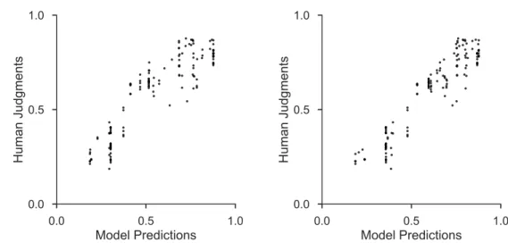
The experimental and model beliefs of cooperativeness were plotted against each other as line graphs to get a high level view of fit, with one line per player and one graph per game sequence. Examples can be seen in Figures 3-1. The experimental and model values per judgments point were also plotted against each other to visualize the level of correlation between the two sets of values, an example of which can be seen in Figure 3-4.

3.3.1

Parameter Optimization

As seen in Section 2.3.2.1, CCAgent depends on two free parameters, beta 𝛽 and decay 𝑑. In order to find the set of parameters that would make our model best fit the human judgments, the model was optimized using SciPy’s optimize method to minimize the root-mean-square error (RMSE) between the experimental means and model beliefs per judgment point.

3.3.1.1 Single Beta and Decay

The optimized fit using 𝛽 = 4.04 and 𝑑 = 0.159 can be seen in Figures 3-1. The fit was generally decent, but there were some values that are repeatedly fit poorly. Take games 10-14, for example, which were double fence games. The blue player was always the one that got stuck at the fence, so its only movement was to continue forward toward the goal. As a result, the model had no indication of how cooperative blue was being, so its value hovered around 0.5 for the entire game sequence. However, the human values tended to be higher, hovering around 0.7 for the entire game sequence. Another instance of this type of ill-fit is in games 23-28, which were PDF games. On the first step both players went for the center and collided, and the blue player won

the collision. At this point, both the human and model beliefs of cooperation were very low. On the next step, the yellow player moved toward its outer goal. Regardless of what the blue player did, this was viewed as a weak signal of cooperation by humans, and the belief always rose to about 0.6. On the contrary, the model still viewed this as competitive-leaning, and the value hovered around 0.4.

In both of these examples, the human and model beliefs followed the same tra-jectories, but the human values tended to be slightly higher. This indicated that, when there was uncertainty of whether a player was behaving cooperatively or com-petitively, humans generally tended to see them as more cooperative. Additionally, it seemed that the human mental model might have been transitioning from competition to cooperation at a separate, higher rate than it was transitioning from cooperation to competition.

3.3.1.2 Asymmetric Decays

To represent the asymmetric transition probabilities, the decay parameter 𝑑 was split into two separate values, 𝑑𝑎 and 𝑑𝑏, so now the transition matrix from step 0 to step

1 is: ⎡ ⎣ 𝑃 (𝐶1) 𝑃 (𝐶₁′) ⎤ ⎦∝ 𝑇 = ⎡ ⎣ 1 − 𝑑𝑎 𝑑𝑏 𝑑𝑎 1 − 𝑑𝑏 ⎤ ⎦ ⎡ ⎣ 𝑃 (𝐶0) 𝑃 (𝐶₀′) ⎤ ⎦ (3.1)

which multiplies out to

𝑃 (𝐶1) ∝ (1 − 𝑑𝑎)𝑃 (𝐶0) + 𝑑𝑏𝑃 (𝐶0′) (3.2)

𝑃 (𝐶₁′) ∝ 𝑑𝑎𝑃 (𝐶0) + (1 − 𝑑𝑏)𝑃 (𝐶0′) (3.3)

To reason about how the two separate values of decay affect the transition prob-abilities, let’s focus on the first element in the resulting matrix, 𝑃 (𝐶1). We know

that 𝑃 (𝐶1) is greater than 𝑃 (𝐶0) for low values of 𝑃 (𝐶0) and is lower than 𝑃 (𝐶0) for

high values of 𝑃 (𝐶0). This is because the decay "decays" values towards the middle.

0 1 2 3 step 0.0 0.2 0.4 0.6 0.8 1.0 Game #0 0 1 2 step 0.0 0.2 0.4 0.6 0.8 1.0 Game #1 0 1 2 step 0.0 0.2 0.4 0.6 0.8 1.0 Game #2 0 1 2 3 step 0.0 0.2 0.4 0.6 0.8 1.0 Game #3 0 2 4 step 0.0 0.2 0.4 0.6 0.8 1.0 Game #4 0 2 4 step 0.0 0.2 0.4 0.6 0.8 1.0 Game #5 0 2 4 step 0.0 0.2 0.4 0.6 0.8 1.0 Game #6 0 2 4 step 0.0 0.2 0.4 0.6 0.8 1.0 Game #7 0 2 4 step 0.0 0.2 0.4 0.6 0.8 1.0 Game #8 0 2 4 6 step 0.0 0.2 0.4 0.6 0.8 1.0 Game #9 0 2 4 step 0.0 0.2 0.4 0.6 0.8 1.0 Game #10 0 2 4 step 0.0 0.2 0.4 0.6 0.8 1.0 Game #11 0 2 4 step 0.0 0.2 0.4 0.6 0.8 1.0 Game #12 0 2 4 6 step 0.0 0.2 0.4 0.6 0.8 1.0 Game #13 0 2 4 6 step 0.0 0.2 0.4 0.6 0.8 1.0 Game #14 0 1 2 3 step 0.0 0.2 0.4 0.6 0.8 1.0 Game #15 0 1 2 3 step 0.0 0.2 0.4 0.6 0.8 1.0 Game #16 0 1 2 3 step 0.0 0.2 0.4 0.6 0.8 1.0 Game #17 0 1 2 3 step 0.0 0.2 0.4 0.6 0.8 1.0 Game #18 0 1 2 3 step 0.0 0.2 0.4 0.6 0.8 1.0 Game #19 0 1 2 step 0.0 0.2 0.4 0.6 0.8 1.0 Game #20 0 1 2 3 step 0.0 0.2 0.4 0.6 0.8 1.0 Game #21 0 1 2 3 step 0.0 0.2 0.4 0.6 0.8 1.0 Game #22 0 2 4 step 0.0 0.2 0.4 0.6 0.8 1.0 Game #23 0 2 4 step 0.0 0.2 0.4 0.6 0.8 1.0 Game #24 0 2 4 step 0.0 0.2 0.4 0.6 0.8 1.0 Game #25 0 1 2 step 0.0 0.2 0.4 0.6 0.8 1.0 Game #26 0 2 4 step 0.0 0.2 0.4 0.6 0.8 1.0 Game #27 0 2 4 step 0.0 0.2 0.4 0.6 0.8 1.0 Game #28 0.00 0.25 0.50 0.75 1.00 0.0 0.2 0.4 0.6 0.8 1.0

Figure 3-1: Plots of each game sequence showing the human (solid) and model (dot-ted) values (using a single 𝛽 and 𝑑) per judgment point per player. (The yellow player is displayed in orange for better visibility.) Games 0-4 are prisoner’s dilemma games, games 5-9 are four-way games, games 10-14 are double fence games, and games 15-28 are PDF games.

𝐶 = 𝑃 (𝐶1) = 𝑃 (𝐶0), which gives us

𝐶 = (1 − 𝑑𝑎)𝐶 + 𝑑𝑏(1 − 𝐶) (3.4)

Solving for 𝐶, we find that 𝐶 = 𝑑𝑏/(𝑑𝑎+ 𝑑𝑏), which we will call the cooperative

decay ratio, or CDR.

When there was a single decay, the CDR was always 𝑑/(𝑑 + 𝑑) = 0.5. This makes sense, as decay pulls values that are further from the middle towards the middle, so values above 0.5 will decrease towards 0.5 and values below 0.5 will increase towards 0.5.

With separate decay values, the CDR is no longer 0.5. We can think of the CDR as the new "middle" that values are pulled towards during the transition. For values of 𝐶0 < CDR, 𝐶0 → 𝐶1 will increase to be closer to the CDR. For values of 𝐶0 >

CDR, 𝐶0 → 𝐶1 will decrease to be further from the CDR. If 𝐶0 = 𝐶𝐷𝑅, then there

is no change from 𝐶0 to 𝐶1.

By setting 𝑑𝑎 and 𝑑𝑏, we can set the CDR and dictate how "cooperative" the

transition from 𝐶0 to 𝐶1 is. If the CDR is high, transitions from 𝐶0 to 𝐶1 will

increase in value more often than they will decrease in value, which means that more values will increase to be more cooperative after the transition. If the CDR is low, transitions from 𝐶0 to 𝐶1 will decrease in value more often than they will increase

in value, which means that more values will decrease, or become more competitive, after the transition.

If we want our model to be more cooperative-leaning in its observations, the CDR should be higher, so 𝑑𝑏 should be higher and 𝑑𝑎 should be lower. This means that,

inversely, if we want our model to be more competitive-leaning, the CDR should be lower, meaning 𝑑𝑏 should be lower and 𝑑𝑎 should be higher. Setting 𝐶′ = 1 − 𝐶, we

find that the decay ratio for 𝐶′ is 𝑑𝑎/(𝑑𝑎+ 𝑑𝑏), which follows the previous statement.

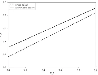
After running the optimization using asymmetric decays, we found 𝑑𝑎 = 0.086

and 𝑑𝑏 = 0.307, and the scatter plot of the values can be seen in Figure 3-4. 𝑑𝑎 is

0.0 0.2 0.4 0.6 0.8 1.0 C_0 0.0 0.2 0.4 0.6 0.8 1.0 C_1 single decay asymmetric decays

Figure 3-2: A comparison between the optimized single decay and optimized asym-metric decays. The dotted line shows the transition from 𝐶0 to 𝐶1 using a single

decay 𝑑 = 0.159, and the solid line shows the transition using the asymmetric decays 𝑑𝑎 = 0.0867 and 𝑑𝑏 = 0.307. The 𝐶1 for asymmetric decays is higher, showing that

the judgments end up being more cooperative-leaning.

a cooperative decay ratio of 0.307/(0.086 + 0.307) = 0.775. This means that after applying the decay, 𝑃 (𝐶1) will generally end up increasing unless it is already quite

high (and even at that point, it doesn’t decrease by much). Figure 3-2 shows how the asymmetric decay values affect the updates to 𝑃 (𝐶1) and 𝑃 (𝐶1′) at different values of

𝑃 (𝐶0) compared to the single decay value 𝑑 = 0.159. This also qualitatively reflects

what we saw from the human attributions when unclear situations were generally perceived to be more cooperative.

Comparing the human and model data points in Figure 3-4, 𝑅 increased from 0.899 to 0.938, 𝑅2 _{increased from 0.809 to 0.879, and the RMSE decreased from}

0.107 to 0.075. By comparing Figures 3-1 and 3-3, we can see that the poorly-fit lines in games 10-14 and 23-28 are also fit much more closely, without the fit being negatively affected in the other games.

0 1 2 3 step 0.0 0.2 0.4 0.6 0.8 1.0 Game #0 0 1 2 step 0.0 0.2 0.4 0.6 0.8 1.0 Game #1 0 1 2 step 0.0 0.2 0.4 0.6 0.8 1.0 Game #2 0 1 2 3 step 0.0 0.2 0.4 0.6 0.8 1.0 Game #3 0 2 4 step 0.0 0.2 0.4 0.6 0.8 1.0 Game #4 0 2 4 step 0.0 0.2 0.4 0.6 0.8 1.0 Game #5 0 2 4 step 0.0 0.2 0.4 0.6 0.8 1.0 Game #6 0 2 4 step 0.0 0.2 0.4 0.6 0.8 1.0 Game #7 0 2 4 step 0.0 0.2 0.4 0.6 0.8 1.0 Game #8 0 2 4 6 step 0.0 0.2 0.4 0.6 0.8 1.0 Game #9 0 2 4 step 0.0 0.2 0.4 0.6 0.8 1.0 Game #10 0 2 4 step 0.0 0.2 0.4 0.6 0.8 1.0 Game #11 0 2 4 step 0.0 0.2 0.4 0.6 0.8 1.0 Game #12 0 2 4 6 step 0.0 0.2 0.4 0.6 0.8 1.0 Game #13 0 2 4 6 step 0.0 0.2 0.4 0.6 0.8 1.0 Game #14 0 1 2 3 step 0.0 0.2 0.4 0.6 0.8 1.0 Game #15 0 1 2 3 step 0.0 0.2 0.4 0.6 0.8 1.0 Game #16 0 1 2 3 step 0.0 0.2 0.4 0.6 0.8 1.0 Game #17 0 1 2 3 step 0.0 0.2 0.4 0.6 0.8 1.0 Game #18 0 1 2 3 step 0.0 0.2 0.4 0.6 0.8 1.0 Game #19 0 1 2 step 0.0 0.2 0.4 0.6 0.8 1.0 Game #20 0 1 2 3 step 0.0 0.2 0.4 0.6 0.8 1.0 Game #21 0 1 2 3 step 0.0 0.2 0.4 0.6 0.8 1.0 Game #22 0 2 4 step 0.0 0.2 0.4 0.6 0.8 1.0 Game #23 0 2 4 step 0.0 0.2 0.4 0.6 0.8 1.0 Game #24 0 2 4 step 0.0 0.2 0.4 0.6 0.8 1.0 Game #25 0 1 2 step 0.0 0.2 0.4 0.6 0.8 1.0 Game #26 0 2 4 step 0.0 0.2 0.4 0.6 0.8 1.0 Game #27 0 2 4 step 0.0 0.2 0.4 0.6 0.8 1.0 Game #28 0.00 0.25 0.50 0.75 1.00 0.0 0.2 0.4 0.6 0.8 1.0

Figure 3-3: Plots of each game sequence showing the human (solid) and model (dot-ted) values (using a single 𝛽 and asymmetric 𝑑) per judgment point per player. The fit compared to Figure 3-1 is improved, indicating that these parameters are reflective of the human mental model.

0.0 0.5 1.0

Model Predictions

Human Judgments

Model Predictions

Human Judgments

Figure 3-4: A comparison of the human versus model values per judgment point using a single decay 𝑑 (left) and asymmetric 𝑑s (right). The correlation using a single 𝑑 was 𝑅 = 0.899, 𝑅2 = 0.809, 𝑅𝑀 𝑆𝐸 = 0.107. The correlation using asymmetric 𝑑s

was 𝑅 = 0.938, 𝑅2 = 0.879, 𝑅𝑀 𝑆𝐸 = 0.0748.

𝛽𝑎 𝑑𝑎 𝛽𝑏 𝑑𝑏 𝑅 𝑅2 RMSE

1 beta, 1 decay 4.04 0.159 – – 0.899 0.809 0.107 1 beta, 2 decays 2.42 0.0867 – 0.307 0.938 0.879 0.0748 2 betas, 2 decays 3.84 0.0899 1.55 0.287 0.942 0.887 0.0708

Table 3.1: A comparison of the optimized values from fitting the CCAgent model with different set of free parameters. Using asymmetric decays had a marked improvement in the fit, but using asymmetric 𝛽s did not.

3.3.1.3 Asymmetric Betas and Decays

We also tried fitting the model using separate 𝛽 values for cooperative and competitive planning, along with the asymmetric decay values. However, the high number of free parameters caused the optimization to take an exceedingly long time to run, without much improvement in the RMSE. A full comparison between the three can be seen in Table 3.1.

3.3.2

Model Comparison

The CCAgent uses two low-level planners, the CoopAgent and the CompeteAgent, for policy generation. To validate that the high-level planner using both the

co-0.0 0.5 1.0

Model Predictions

Human Judgments

Model Predictions

Human Judgments

Figure 3-5: The fit between human and model values per judgment point for the lesioned models (Cooperate-Random on the left, and Random-Compete on the right). The values are quite scattered, with no strong positive correlation.

operate and compete modes of planning was indeed the most representative of the human mental model, the CCAgent was compared against two lesioned models. The Cooperate-Random Agent used the CoopAgent and RandomAgent, and the Random-Compete Agent used the RandomAgent and Random-CompeteAgent (see Section 2.3.1 for a detailed explanation of the different low-level planners).

Each agent’s parameters 𝛽, 𝑑𝑎, and 𝑑𝑏 were optimized by minimizing the RMSE

between the experiment and model values as in Section 3.3.1. The full results of the optimized parameters can be see in Table 3.2. Even though these lesioned models were optimized, the fit was still evidently worse - this can be seen through the 𝑅, 𝑅2_,

and RMSE values in Table 3.2 and the scatter plots in Figure 3-5.

Through these comparisons, we can see that the high-level planner must use both cooperative and competitive planning in order to attribute cooperative and compet-itive behavior in a manner similar to humans. Of the models used in the attribution experiment, the CCAgent is the most representative of the mental model humans use when attributing cooperative intention and behavior.

𝛽𝑎 𝑑𝑎 𝑑𝑏 𝑅 𝑅2 RMSE

Cooperate-Compete (CC) Agent 2.42 0.0867 0.307 0.938 0.879 0.0748 Cooperate-Random Agent 4.66 0.215 0.0781 0.820 0.673 0.120 Random-Compete Agent 3.90 0.0290 0.463 0.770 0.593 0.139 Table 3.2: A comparison of the optimized values using the CCAgent, Cooperate-Random Agent, and Cooperate-Random-Compete Agent and how well each model fit to the experimental data. Clearly, the CCAgent outperformed both lesioned models.

3.4

Discussion

Examining the line graphs in Figure 3-3 and the flowcharts in Appendix A, we can see people generally attributed behavior to the players in a way that we expected and that people were able to make meaningful judgments based on just a single state-action sequence. Games 0-4 were sequences played on the prisoner’s dilemma game described in Section 2.2.1, and games 5-9 were sequences played on the the four-way game described in Section 2.2.2. It is clear that participants understood which movements were cooperative and competitive, rating highly when a player waited or both players reached their goals at the same time, and rating lowly during collisions or when a single player reached their goal first.

Games 4 and 9 in particular show instances of miscoordinated cooperation. In game 4, the players collide in the center square, which looks like competitive behav-ior. In game 9, both players wait a turn before the intersection and then both try to move into the intersection on the next turn. In both games, the collision is seen as quite competitive, even in game 9 when both players had waited on the previous turn. This indicates that, attribution-wise, any signs of disharmony look quite com-petitive, even if it was a mistake of coordination. Eventually the players recover and end up in their goals at the same time, and both are seen as cooperative again. This reveals that seemingly competitive movements in the middle, which can be chalked up to miscoordination, do not affect the overall assessment that both players were behaving cooperatively. This reinforces the statement from Section 1.2.2, where mis-coordination is simply a possible component of cooperation and not necessarily a detractor.

Games 10-28 all involved fences, which resulted in final outcomes that were in-congruous to the actual intention of the player. However, the participants were able to judge the behavior based on the intention - a competitive outcome did not take away from cooperative intent, and vice versa. This is particularly noticeable in games 15-28, which were PDF games. As seen in Figures A-4 and A-5, the fences resulted in 2-3 different outcomes per identical game sequence. However, looking at the line graphs in Figure 3-3, we can see that for each identical game sequence (disregarding the final outcome), the participants’ judgments were very similar. This demonstrates that the human mental model does indeed look at the entire sequence of movements when assessing cooperative behavior and not just at the final outcome. Therefore, it is important that our model is able to assess the entire sequence and make judgments at each point rather than purely looking at the final outcome.

3.5

Future Optimizations

There are a few steps that can be taken to further improve the fit of the model. There are a lot of judgment points that are equivalent in terms of the states and actions leading up to that point. It would be useful to average judgments with duplicate histories to decrease the noise and redundancy of the data. This would also likely improve the fit of the model to the data.

We made the assumption that people’s priors were 0.5, but in reality people could come in predisposed with a belief of how cooperative people generally are. The prior could potentially be pulled out as a free parameter and optimized upon as well.

Finally, we can test the robustness of the model across different types of games. First, we could re-run the attribution experiment with completely new game se-quences. Then, we could use the currently optimized model to make judgments on the new game sequences. By comparing these new model predictions with the new experimental data, we can test how good of a predictor the model is on games that were not used for its optimization. We can also see if the model overfit to the previous experimental data and iterate on which free parameters should be used for

Chapter 4

Two-Player Experiment

We also ran a two-player experiment where participants played 15 repeated rounds of the prisoner’s dilemma with fences (PDF) game detailed in Section 2.2.1 against another participant. This game combined both the features of a social dilemma and tested for intention versus outcome. The purpose of this experiment was to gain insight on how actual humans would play this game, if it aligned with our expectations of what would happen, and if our model would be able to fit these human-selected movements. This experiment was also run on Amazon Mechanical Turk (MTurk) with 92 participants, with 24 pairs of participants completing all 15 rounds of the game.

4.1

Experimental Design

The two-player experiment began with a tutorial that taught users the game rules described in Section 2.1 through a series of interactive slides. Users had to select and make moves on the grid in order to complete the tutorial and get familiar with how to play the game. To describe the collisions, the tutorial used the same playback mechanism as the attribution experiment in Chapter 3. Users were also able to navigate back and forth throughout tutorial slides in case they wanted to reread or retry anything. See https://youtu.be/ZEHFByfoi7s for a video of the two player experiment tutorial.