Low temperature devices (FDSOI, TriGate) junction optimization for 3D sequential integration

(1)

HAL Id: tel-01303732

https://tel.archives-ouvertes.fr/tel-01303732

Submitted on 18 Apr 2016

HAL is a multi-disciplinary open access archive for the deposit and dissemination of sci-entific research documents, whether they are pub-lished or not. The documents may come from teaching and research institutions in France or abroad, or from public or private research centers.

L’archive ouverte pluridisciplinaire HAL, est destinée au dépôt et à la diffusion de documents scientifiques de niveau recherche, publiés ou non, émanant des établissements d’enseignement et de recherche français ou étrangers, des laboratoires publics ou privés.

Low temperature devices (FDSOI, TriGate) junction

optimization for 3D sequential integration

Luca Pasini

To cite this version:

Luca Pasini. Low temperature devices (FDSOI, TriGate) junction optimization for 3D sequential integration. Micro and nanotechnologies/Microelectronics. Université Grenoble Alpes, 2016. English. �NNT : 2016GREAT017�. �tel-01303732�

(2)

THÈSE

Pour obtenir le grade de

DOCTEUR DE L’UNIVERSITÉ GRENOBLE ALPES

Spécialité : Nano électronique et Nano technologie

Arrêté ministériel : 7 août 2006 Présentée par

Luca PASINI

Thèse dirigée par Gérard GHIBAUDO et

codirigée par Perrine BATUDE et Mikael CASSE préparée au sein du CEA LETI et STMicroelectronics dans l'École Doctorale Electronique, Électrotechnique, Automation et Traitement du Signal

Optimisation des jonctions de dispositifs

(FDSOI,

TriGate)

fabriqués

à

faible

température

pour

l’intégration

3D

séquentielle

Low temperature devices (FDSOI, TriGate)

junction optimization for 3D sequential

integration

Thèse soutenue publiquement le 15 Mars 2016, devant le jury composé de :

M. Francis CALMON

Professeur à l’INSA, Lyon (Président)

M. Emmanuel DUBOIS

Directeur de Recherche, CNRS/IEMN (Rapporteur)

M. Fuccio CRISTIANO

Chargé de recherche, CNRS/LAAS (Rapporteur)

M. Gérard GHIBAUDO

Directeur de recherche à l’IMEP/INPG (Directeur de thèse)

Mlle. Perrine BATUDE

Ingénieur, Docteur, CEA-LETI (Encadrant)

M. Mikael, CASSE

Ingénieur, Docteur, CEA-LETI (Encadrant)

M. Michel, HAOND

(3)

1

Acknowledgments

If I am writing this Ph.D. thesis, it means that I really have to thank a lot of people. First of all, my Ph.D. director Gérard Ghibaudo and my supervisor at STMicroelectronics Michel Haond that accept to supervise this thesis.

I would like to thank my two LETI supervisors Mikael Casse and Perrine Batude. The first, for his efficiency in everything concerning the electrical characterization. The second…for everything. We have worked every day for three years together, I learnt millions of things and, most important, a method of working. I think we have done a good work together; it has been an honor to be your student.

I would like to thank the entire LICL lab from Maud, for her energy and passion as lab manager, to all the technicians Bernard, Claude, Michel, Laurent, Marie-Pierre and the engineers as well: Louis, Cyrille, Yves, Olivier, Sylvain, Hervé, Christophe. It has been nice to be in this lab.

I want to dedicate a special section for the CoolCube team: Perrine, Claire, Laurent, Paul, Louis, Fabien, Vincent. It has been a pleasure to work in this team. I wish all the best to Jessy that is going to continue the work of my thesis. A special thanks as well to Pierette, Benoit Sklénard, Benoit Mathieu Anthony and Sébastien for their support in simulation. Thank you to Flavia for her huge work as CoolCube team-member infiltrated in DTSI.

A special thanks to Valérie and Nils that followed the advancement of our lots in ST. Thank you for your patience, interest, reactivity and efficiency. It has been a pleasure to work with you.

Thank you to all the people from STMicroelectronics: David Barge, Vincent Mazzocchi, Sonarith Chhun, Sebsatien Lagrasta, Francesco Abbate, Romain Duru, Sylvain Joblot, Rémy Berthelon, Olivier Weber and Vincent Barral always available to help me.

Several people helped me in the realization and characterization of the devices that I have analyzed in this thesis, I am sure I am going to forget someone, but I can try: Frederic Mazen, Pascal Besson, Vincent Delaye, Dominique Lafond, Christophe Licitra, Sebastien Kardiles.

Thank you as well to the people that supported in me in the electrical characterization: Giovanni, Fabienne, Denis, Antoine, Xavier.

Now it is the turn of all the other Ph.D. students (or post-docs)! I do not know if all of you deserve to be in this list, because I have met several brutte persone during years. However, I am writing these acknowledgments during Christmas holidays, so I am happy to thanks everybody starting from our fantastic office: Julien, Mathilde and Alexandre. I wish the best for your future. Same office, but different time: Simeon, Anthony, Heimanu and Gabriele. You have helped me a lot when I was just arrived. Thank you! And thank you to all the other guys as well for a lot of funny moments spent together: José, JulienD, Fabien, Vincent, Loic, Daniele, Marinela, Giorgio, Rémy, Issam, Anouar, Lina, Blend, Giulio, Elodie.

(4)

2

A special thank you to the Italian group: we shared so many moments in these years! Niccolo’, Ilaria, Leoncino, Fede, Valeria, Michael, Leandro, I hope to continue to be in contact with you for the rest of my life.

Thank you to my family for their support and to my friends that even if I am not in Italy from three years, every time that I come back I feel like I have never left them.

I have arrived in Grenoble three years ago alone, I did not speak French, I did not know anything about process integration, everything looked so complicated. Three years later, I simply think that this has been one of the best periods of my life. Thank you.

(5)

3

List of figures

I.1 Description of parallel integration process ﬂow I.2 Description of 3D sequential integration process ﬂow

I.3 Summary of thermal budgets tested on 14nm FDSOI technology with preserved N &PFET ION -IOFF performance.

I.4 Description of the 3D sequential integration scheme process

I.5 TEM observation of stacked transistor fabricated with the 3D sequential integration scheme

1.1. Schematic representation of ion implantation.

1.2. SPER mechanism consists in a re-crystallization layer by layer starting from the crystalline seed

1.3. RNG process consist in the nucleation of small agglomerates that further expand into crystallites

1.4. Maximum active concentration for boron, arsenic and phosphorus as a function of annealing temperature

1.5. Scheme of full sheet SOI sample used for SPER analysis.

1.6. Mobility-concentration behavior at thermodynamic equilibrium for boron, phosphorus and arsenic as a function of the concentration [Masetti 83]. 1.7. TEM image of Sample 5 after phosphorus high dose implantation. 1.8. Sheet resistance measurements for samples described in Table 1.1. 1.9. Resistivity values for samples described in Table 1.1.

1.10. Dose and mobility measurements results for As samples.

1.11. Arsenic profiles after 2 minutes at 600°C extracted by KMC simulation. 1.12. Hall Mobility measurements results for P samples.

1.13. Phosphorus profiles after 2 minutes at 600°C annealing extracted by KMC simulation 1.14. Comparison between the electron mobility versus carrier concentration curves at

1050°C thermodynamic equilibrium [Masetti 84] and the experimental points at low dopant dose (S4 and S6).

1.15. Sheet resistance – temperature curve for the in-situ experimental test of post annealing on S3.

1.16. Sheet resistance percentage variation after post annealing of 30 minutes at 550°C. 1.17. SPER optimization challenges.

1.18. Sheet resistance values measured on samples reported in Table 1.2 for p-type doping.

1.19. Boron profiles after 2 minutes at 600°C annealing extracted by KMC simulation. 1.20. Phosphorus concentration profile obtained by KMC simulations.

1.21. Boron concentration profile obtained by KMC simulations.

1.22. Experimental results of the in-situ ellipsometry annealing showing the evolution of the amorphous silicon thickness as a function of annealing time for a 550 °C anneal. 1.23. Experimental SPER rates obtained from in-situ ellipsometry annealings performed at

temperatures from 450 °C to 600 °C, as a function of the simulated phosphorus concentrations.

1.24. Experimental SPER rates obtained from in-situ ellipsometry annealings performed at temperatures from 450 °C to 600 °C, as a function of the simulated boron

concentrations. 14 14 15 16 16 19 21 21 22 23 24 25 26 26 27 27 28 28 28 29 29 31 32 32 34 34 34 35 35

(8)

6

1.25. Optimal boron and phosphorus concentrations to enhance the SPER rate as a function of the annealing temperature. The dashed lines are a simple linear fit of the experimental points.

1.26. Comparison between SIMS and simulation profile for phosphorus sample. 1.27. Comparison between SIMS and simulation profile for boron sample.

1.28. Simulated concentration-depth profile of the as-implanted P ions superimposed to the TEM image of the w/SiO2 sample. This implantation resulted in a ~17 nm thick

a-Si layer recovered by ~2 nm of native a-SiO2, leaving 4 nm of crystalline seed.

1.29. Average sheet resistance values for both w/SiO2 and w/o/SiO2 phosphorus samples

annealed at different thermal budgets.

1.30. Average sheet resistance values for both w/SiO2 and w/o/SiO2 boron samples

annealed at different thermal budgets.

1.31. Cross-section HRTEM images of samples annealed at 450 °C for 60 min.

1.32. In-situ ellipsometry 450 °C annealing of P implanted samples with (w/SiO2) and without (w/o/SiO2) the oxide layer. The amorphous silicon thickness is shown as a function of the annealing time.

1.33. In-situ ellipsometry 450 °C annealing of B implanted samples with (w/SiO2) and without (w/o/SiO2) the oxide layer.

1.34. Simulation of oxygen concentration inserted into the 22 nm Si top film by recoil due to the of Ge+B and P ion implantations. The shadowed region corresponds to the 1 nm thick SiO2 that is assumed to be present on the sample surface.

1.35. Sheet resistance of B and P samples implanted with the SiO2 superficial layer as a

function of the non-recrystallized amorphous layer thickness measured by ellipsometry after SPER annealings at 600 °C, 500 °C and 450 °C.

2.1. nMOS transistor scheme in ON state. 2.2. IDS(VGS) nMOS characteristic.

2.3. IDS (VDS) characteristic for nMOS. The line VDS=VGS-VT divides the triode mode from

saturation mode.

2.4. Schematic representation of Bulk and FDSOI MOSFET devices. Typical dimensions of FDSOI device for 28nm node are reported as well.

2.5. Standard process flow for 28nm FDSOI technology.

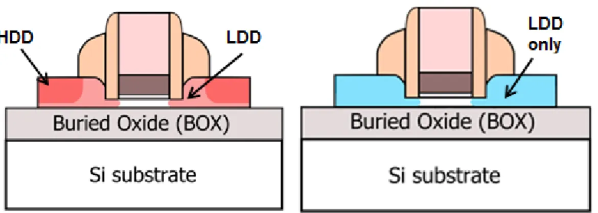
2.6. Difference in doping strategy for high temperature and low temperature devices. 2.7. Process flow comparison between high temperature (a) and low temperature (b)

devices.

2.8. One dimensional phosphorus chemical profile. 2.9. One dimensional arsenic chemical profile.

2.10. ION-IOFF trade-off for nMOS high temperature device, considered as reference and

low temperature devices. Performance degradation is show for low temperature devices.

2.11. Access resistance extraction by Y function method for high temperature and low temperature devices. The resistance values reported, correspond to the half of the total resistance (drain resistance).

2.12. Access resistance contributions scheme.

2.13. The region below the first spacer is difficult to dope for low temperature dopants activation for two reasons: (i) difficulty in creating amorphous region, (ii) no dopant diffusion for low temperature activation.

2.14. Dopant concentration under first spacer extracted from KMC simulation for high temperature device.

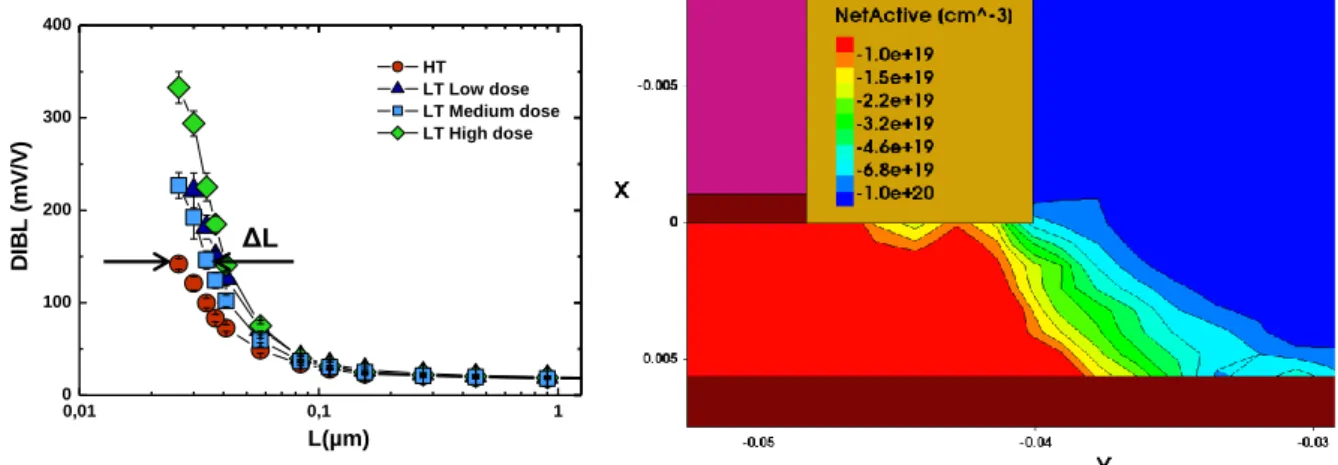
2.15. Dopant concentration under first spacer extracted from KMC simulation for low temperature device with phosphorus doping device. RSPA is also defined.

36 37 37 38 40 40 41 42 42 42 43 47 48 48 50 53 53 54 55 55 56 56 57 57 58 58 58

(9)

7

2.16. Dopant concentration under first spacer extracted from KMC simulation for low temperature device with arsenic doping device.

2.17. 5x1019_at/cm3_{iso-concentration evolution of high temperature and low temperature}

devices obtained by KMC simulation.

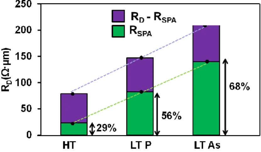
2.18. RSPA contribution extracted by SDEVICE simulation. The percentage of RSPA on total

drain resistance (experimentally measured) is also shown. 2.19. Physical (Lphys) an electrical (Lelec) gate length definition.

2.20. Overlap/underlap configuration definition obtained by simulation results.

2.21. DIBL behavior for different gate lengths for high temperature and low temperature devices.

2.22. Carrier mobility at low electric field for different gate lengths extracted for high temperature and low temperature devices.

2.23. EOT for different gate lengths extracted for high temperature and low temperature devices.

2.24. ION-IOFF trade-off for pMOS high temperature device, considered as reference and

low temperature devices.

2.25. Access resistance extraction by Y function method for high temperature and low temperature devices. The resistance values reported, correspond to total access resistance (drain and source resistance).

2.26. DIBL at different gate lengths for high temperature and low temperature devices. 2.27. Dopant concentration under first spacer extracted from KMC simulation for low

temperature device with low doping dose.

2.28. Dopant concentration under first spacer extracted from KMC simulation for low temperature device with medium doping dose.

2.29. Dopant concentration under first spacer extracted from KMC simulation for low temperature device with high doping dose.

2.30. Carrier mobility at low electric for different gate lengths.

2.31. θ2-β plot. Under the hypothesis of RSD(VGS)=R0 + λ(VGS-VT), λ is represented by the

slope of this graph.

2.32. Carrier mobility extraction considering ~/VGS behavior of the access resistance.

2.33. Carrier mobility corresponding to low temperatures device with low dose doping for different values of 𝜎.

2.34. TEM cross section of a tested low temperature FDSOI device.

2.35. Normalized ION.IOFF performance of LT FDSOI N- & P-devices compared with HT-POR,

for different implantation tilt angle.

2.36. Comparison of Lot 1 and LOT 2 nMOS performance for the HT reference.

2.37. TEM cross section of high temperature device for lot 1 and lot 2. The difference in first spacer thickness is highlighted.

2.38. ION-IOFF performance benchmark of LT planar devices with literature data (all LT

activation methodologies confounded).

2.39. RON - DIBL measurements for high temperature and low temperature nMOS devices.

2.40. Junction simulation by SPROCESS KMC.

2.41. TEM micrograph and a map of the out-of-plane component of strain on patterned sSOI substrate.

2.42. TEM cross section showing lateral recrystallization at 550°C after patterned full film amorphization. Defective {111} recrystallization is observed.

2.43. Example of amorphous/crystalline interface obtained b 3D simulation

2.44. Amorphous-crystalline interface roughness estimation versus amorphized thickness for different species (Ge and P) extracted by SPROCESS KMC simulation.

2.45. RSPA-TSEEDMIN trade-off for FDSOI device at low temperature with extension last

integration. 58 59 60 61 61 62 62 63 63 64 64 65 65 66 66 68 68 69 69 70 70 71 71 71 72 72 74 74 75 75 76

(10)

8

2.46. RSPA-TSEEDMIN trade-off for FDSOI device at low temperature with extension first

integration.

2.47. KMC simulation of junction profile for extension last and extension first integration. 2.48. Schematic representation of FD, TriGate and FinFet on insulator geometries. 2.49. TEM cross section of low temperature TriGate device.

2.50. TEM cross section in lateral direction of low temperature TriGate device.

2.51. ID-VG characteristics of low temperature N&P-Trigate with extension last normalized

by WEFF= WTOP+2×HNW.

2.52. ID-VD characteristics of low temperature N&P-Trigate with extension last integration

normalized by WEFF= WTOP+2×HNW.

2.53. ION-IOFF performance benchmark of low temperature Trigate N&P devices with

literature data. WEFF normalization used for this work.

2.54. Experimental extraction of access resistance for high temperature and low temperature TriGate devices.

2.55. Junction simulation by SPROCESS KMC for HT/LT Trigate devices.

2.56. Trigate low temperature junction figure of merit: RSPA-TSEED MIN trade-off for extension

last scheme.

2.57. Trigate low temperature junction figure of merit: RSPA-TSEED MIN trade-off for extension

last scheme.

2.58. FinFET low temperature junction figure of merit: RSPA-TSEED MIN trade-off.

3.1. Process flow for 14nm FDSOI technology.

3.2. TEM cross section for nMOS and pMOS fabricated with the POR process 14nm FDSOI.

3.3. Low temperature extension first scheme. Only the process steps that are different from standard flow presented in Figure 3.2 are here illustrated.

3.4. Simulated structure for doping conditions definition in extension first scheme. 3.5. Phosphorus 1D profile, after xFirst implant.

3.6. Boron 1D profile, after xFirst implant.

3.7. Amorphization level for different germanium pre-amorphization doses, with phosphorus doping.

3.8. Amorphization level for different germanium pre-amorphization doses, with boron doping.

3.9. TEM observation of amorphized region after Ge+P extension First implant. 3.10. TEM observation of amorphized region after Ge+B extension First implant.

3.11. Simulated structure for doping conditions definition in Extension First scheme with nitride capping.

3.12. Phosphorus 1D profile, after extension first implant through nitride capping liner. 3.13. Boron 1D profile, after Extension First implant through nitride capping liner.

3.14. TEM observation of amorphized region after Ge+P extension First implant on Si film through SiN capping.

3.15. TEM observation of amorphized region after Ge+B extension First implant on SiGe film through SiN capping.

3.16. TEM cross section of Boron doped SiGe film after 5min 500°C. 3.17. TEM cross section of Boron doped SiGe film after 10min 640°C.

3.18. RSHEET measurement of boron Implant on SiGe film onto 300 mm wafer.

3.19. SiN thickness variation on a 300 mm wafer measured by ellipsometry.

3.20. Active doping profile obtained by ECV technique in comparison to chemical profile (simulation).

3.21. Top view observation post SiC:P epitaxy for different PAI conditions on isolated structures. The epitaxial quality improves if the PAI dose is reduced.

77 77 77 78 78 78 78 79 80 80 80 87 87 89 90 90 90 91 91 91 91 92 93 93 93 93 94 94 95 95 96 98 98 99 99

(11)

9

3.22. Top view observation on ring oscillators structures after n-type epitaxy for different implantation conditions.

3.23. GOF ellipsometry measurement post SiC:P epitaxy on 17 wafer sites. 3.24. SiC:P epitaxy thickness by ellipsometry.

3.25. RSHEET measurement on Bulk and SOI structures for splits described in Table 3.1.

3.26. Top view observation post p-type epitaxy on Ring Oscillator structures. 3.27. GOF ellipsometry measurement post SiGe:B epitaxy on SiGeOI structures.

3.28. Total SiGe:B epitaxy and SiGe film thickness by ellipsometry on SiGeOI structures. 3.29. GOF ellipsometry measurement post SiGe:B epitaxy on bulk strcutures.

3.30. SiGe:B epitaxy thickness by ellipsometry on bulk strcutures.

3.31. RSHEET measurement on Bulk and SOI unciliced structures for splits described in Table

3.1.

3.32. TEM observation of nMOS FDSOI device fabricated with extension first integration. 3.33. ION-IOFF performance of Low Temperature Extension First nFET devices compared

with HT-POR 14FDSOI for different PAI conditions. 3.34. Access resistance extraction of nFET devices.

3.35. TEM observation of full sheet samples implanted with phosphorus no PAI conditions. 3.36. RSHEET measurement on Bulk and SOI siliced n-type structures for splits detailed in in

Table 3.1.

3.37. RON vs DIBL at 20nm channel length for splits detailed in in Table 3.1.

3.38. Carrier mobility at low electric field versus gate length for nFET devices on Table 3.1. 3.39. Theta 2 – beta plot for nMOS extension first devices

3.40. ION-IOFF performance of Low Temperature Extension First pFET devices compared

with HT-POR 14FDSOI for different PAI conditions. 3.41. Access resistance extraction of pFET devices.

3.42. RSHEET measurement on Bulk and SOI siliced p-type structures for splits detailed in in

Table 3.2.

3.43. RON vs DIBL at 20nm channel length for splits detailed in in Table 3.2.

3.44. DIBL for different channel lengths and ΔL extraction for pFET devices on Table 3.2. 3.45. Carrier mobility at low electric field versus gate length for pFET devices on Table 3.2.

Dashed lines consider ΔL correction.

4.1. Cross sectional TEM results of As implanted at (a) RT, (b) 300°C and (c) 600°C [Onoda14].

4.2. TEM observation after a) room temperature implantation; b) heated implantation [Wood13].

4.3. Phosphorus profiles obtained by KMC simulation for different implantation temperatures (RT, 300°C, 500°C). Significant differences in profile shape are observed.

4.4. Dopant profile comparison between SIMS and simulation for a) Boron; b) Phosphorus; c) Arsenic hot implantation (500°C).

4.5. Doping profiles of implant conditions detailed in Table 4.1.

4.6. Carrier concentration and mobility measured by Hall effect and deduced form sheet resistance measurement for SOI sample with boron heated implantation.

4.7. Sheet resistance measurements post phosphorus hot implantation on bulk and SOI substrates.

4.8. Carrier concentration and mobility measured by Hall effect and deduced form sheet resistance measurement for SOI sample with phosphorus heated implantation. 4.9. Arsenic doping profiles of implant conditions detailed in Table 4.2.

4.10. Sheet resistance measurements post Arsenic hot implantation on Bulk and SOI substrates. 100 101 101 101 102 102 103 103 104 104 104 104 104 105 105 105 106 106 106 106 108 109 109 110 110 113 113 114 115 115 116 117 117 117 118

(12)

10

4.11. Carrier concentration and mobility measured by Hall effect and deduced form sheet resistance measurement for SOI sample with arsenic heated implantation.

4.12. Sheet resistance measurements post boron hot implantation and SPER activation. 4.13. Sheet resistance measurements post arsenic hot implantation and SPER activation. 4.14. Comparison of sheet resistance measurements on SOI substrate after SPER

activation with room temperature implant, SPER with hot implantation and heated implantation only.

4.15. schematic process flow of extension last with heated implantation in combination with amorphization and dopant activation by SPER.

4.16. TEM observation of a pMOS FDSOI fabricated using the process flow presented in Figure 4.13.

4.17. Total boron concentration after heated implantation for the first simulated condition.

4.18. Total boron concentration after heated implantation for the second simulated condition.

4.19. One-dimensional profile of boron implantation conditions chosen for electrical device.

4.20. Amorphous/crystalline zone obtained by simulation with the germanium implantation at 11KeV.

4.21. ION-IOFF trade-off performance for hot implant split with respect to high temperature

devices and low temperature devices with RT implant.

4.22. Access resistance extraction by Y function method. In this case, the method completely fails.

4.23. Access resistance extraction by RTOT(L) method. Huge access resistance degradation

if found for hot implant split.

4.24. DIBL behavior for different gate lengths. DIBL reduction for hot implant device indicates underlap configuration.

4.25. Carrier mobility at low electric filed extraction.

4.26. Total phosphorus concentration obtained by simulation in the region below the first spacer.

4.27. ION-IOFF trade-off for low temperature devices with hot implantation in comparison

with high temperature POR and low temperature device with RT implantation. 4.28. TEM observation for nMOS fabricated by extension last integration and a) RT

implantation b) hot implantation followed by SPER.

4.29. Schematic representation of the two resistance components associated to the salicide/silicon contact resistance [Dubois 02].

4.30. IDS (VGS) of two n-type device with same geometry on the same wafer. One first

typical MOSFET behavior and the other Schottky behavior.

4.31. Device configuration depending on the position of salicide/silicon interface: a) MOSFET device; b) MOSFET device with performance degradation due to high salicide/silicon contact resistance; c) Schottky device.

4.32. Silicon consumption after nitride removal, for samples subjected to heated implantation.

4.33. TEM observation on n-type FDSOI with extension first integration and heated implantation.

4.34. Schematic process flow for implantation and epitaxial steps in the extension first integration applied on TriGate devices with hot implantation.

4.35. TEM observation of an n-type TriGate device fabricated with the process flow illustrated in Figure 4.32.

4.36. Simulated structure of TriGate device.

4.37. Total boron concentration after hot implantation obtained by KMC simulation focusing on the region below the first spacer.

118 119 119 119 121 121 122 122 123 123 124 124 125 125 126 127 127 127 127 128 129 130 131 132 132 134 134

(13)

11

4.38. ION-IOFF trade-off for p-type low temperature devices with hot implantation in

comparison with high temperature process of reference.

4.39. Access resistance degradation for p-type hot implant split compared to process of reference.

4.40. Sheet resistance measurements on siliced active zone with and without contact resistance for hot implant split and POR.

4.41. RTOT-DIBL trade-off for low temperature devices with hot implantation in comparison

with high temperature POR.

4.42. DIBL at different gate lengths for low temperature devices with hot implantation in comparison with high temperature POR.

4.43. Carrier mobility at low electric field. No variations are observed between high temperature device and low temperature with hot implant.

4.44. Total phosphorus concentration after hot implantation obtained by KMC simulation focusing in the region below the first spacer.

4.45. Active phosphorus concentration after hot implantation obtained by KMC simulation focusing in the region below the first spacer.

4.46. ION-IOFF trade-off for n-type low temperature devices with hot implantation in

comparison with high temperature POR.

4.47. Access resistance degradation for n-type hot implant split compared to POR. 4.48. Sheet resistance measurements on siliced active zone with and without contact

resistance for hot implant split and POR.

4.49. DIBL behavior for different gate lengths for low temperature devices with hot implantation in comparison with high temperature process of reference.

4.50. Carrier mobility at low electric field. No variations appear between high temperature device and low temperature with hot implant.

135 135 136 136 136 136 137 137 138 138 139 139 139

(14)

12

List of tables

1.1 Samples description with type of annealing, dopants implanted doses and crystalline seed thickness

1.2 Samples description with type of annealing, dopants implanted doses and crystalline seed thickness.

2.1. Summary of the advantages and disadvantages for Xlast_{, full amorphization, partial}

amorphization and X1st_integration.

2.2. Minimum thickness seed calculation for extension last and extension first integrations. 3.1. Splits details of nMOS devices.

3.2. Splits details of pMOS devices.

4.1. Implant conditions corresponding to doping profiles of Figure 4.2. 4.2. Implant conditions details for arsenic hot implantations.

4.3. Implantation condition details for extension first integration on TriGate devices.

25 31 73 74 89 102 115 117 133

(15)

13

Introduction and context of this work

Since the introduction on the market of the first microprocessor by INTEL in 1971, the reduction of the MOSFET transistor dimensions has been the driving force of the growth of the semiconductor market. This scaling trend has followed the so called Moore’s law [Moore 65], which predicts that the number of transistors per Integrated Circuits (IC) is doubled every 18 months. This prediction has been basically respected until nowadays, for example with the fabrication of the 28 nm technological node with the FDSOI planar technology by STMicroelectronics and even the 14 nm FinFET technology proposed by INTEL. These ultra-scaled dimensions are approaching to both technological and physical limits concerning the device fabrication and operation: the miniaturization of device feature requires more complex photolithography and etching systems, raising the production cost [Khorram12]. Reliability and variability [Kuhn 11], are also becoming serious concerns as device dimensions scale down. The scaling has also given rise to the increase of parasitic phenomena such as short channel effects (SCE). As a consequence, solutions have to be developed in order to overcome these problems. In particular, for actual technology nodes, new architectures have been introduced such as planar fully depleted Silicon on Insulator (FDSOI) devices or multiple gates FETs [Kuhn 11]. Planar FDSOI, TriGate and FinFET architectures are considered up to 10 nm node depending on the semiconductor company strategy. Beyond, multiple gates or gate all–around FET [Bangsaruntip 09] or even the introduction of non-based silicon technology such as III-V materials [Czornomaz 13], might be mandatory to ensure high performance and gate control of the channel.

In addition, with the increase of the number of transistor, the interconnection length increases more and more becoming one of the main sources of circuit performance limitation rather than the single transistor performance. Therefore, alternative solutions also have to be found in terms of circuit design.

I.1 3D Sequential Integration

An alternative path to planar scaling can be brought by a 3D integration scheme which consists in stacking the transistor levels rather than reducing the devices dimensions. 3D integration can refer to 3D parallel integration, where different chips are processed independently and stacked vertically afterward as shown schematically in Figure I.1. The connection between the stacked layers can be, for example, Through– Silicon Vias (TSV).

(16)

14

Figure I.1: Description of parallel integration process ﬂow. (a) Wafers are processed separately (b) stacked and the contacted afterwards.

However, this method is limited to connecting blocks of a few thousands of transistors and the interconnection density is limited by the alignment precision of bonding [Koyanagi 09]. An alternative technique is represented by the 3D sequential integration [Batude 11a]. In this integration scheme, transistor layers are processed sequentially and the stacked layers can be connected at the transistor scale as shown schematically in Figure I.2. This integration offers higher integration density thanks to its much higher alignment accuracy (approximately 10 nm against 0.5 μm for parallel integration), making full use of the third dimension.

Figure I.2: Description of 3D sequential integration process ﬂow where transistor layers are processed sequentially. (a) The bottom transistor layer is processed, (b) top active zone is fabricated, (c) first lithographic pattern of the top layer (d) the layers are then contacted.

One of the main challenges of the 3D sequential integration is the development of a low temperature process flow for the top transistor level in order to avoid the degradation of the bottom one. The most critical process step for the top transistor level fabrication is the dopant activation that is

(17)

15

conventionally performed by spike annealing at temperature higher than 1000 °C. This thermal budget is not acceptable for the integrity of the bottom level. In [Fenouillet 14] it is reported that bottom transistor performance stability is dependent on the considered technology and, for example, is maintained for annealings at 500 °C for 5 hours and 550 °C for 2 hours in the case of a 14 nm FDSOI. It is worth noticing that both temperature and time are important for the definition for the maximum thermal budget. Therefore, short anneals, such as DSA (Dynamic Surface Anneal) laser, shows negligible performance degradation at 800 °C for 0.3 ms [Batude 15]. For this reason, laser anneal in the range of nanoseconds appears a promising candidate for dopant activation of the top level even though the local temperature can reach 1200 °C.

One of the possible options considered is to activate the dopants through solid phase epitaxial regrowth (SPER), which mechanism will be described later, using annealing temperature below 600 °C instead of conventional spike anneals. This is compatible with a 3D sequential integration scheme as shown in Figure I.3. The work of this thesis will focus on low temperature dopant activation by SPER.

Figure I.3: Summary of thermal budgets tested on 14nm FDSOI technology with preserved N &PFET ION-IOFF performance [Batude 15].

CEA-LETI named the 3D sequential integration scheme with the low temperature process for the top transistor level as CoolCube technology. The simplified CoolCube process flow to integrate sequentially two transistor levels is illustrated schematically in Figure I.4. The bottom transistor is processed with a conventional high temperature thermal budget (Figure I.4a). Then, the top film layer is obtained via a low temperature direct bonding of an SOI substrate enabling the full transfer of a monocrystalline silicon layer (Figure I.4b). Finally, the top transistor is fabricated using a low temperature budget process (Figure I.4c). Figure I.5 shows a Transmission Electron Microscopy (TEM) cross-section image of two stacked transistors after the source and drain epitaxial growth of the top transistor level [Batude 15]. 1n 1µ 1m 1 1k 1M 200 400 600 800 1000 1200 Temper ature (°C ) Anneal duration (s) Stability validated Laser local annealing

(18)

16

Figure I.4: Description of the 3D sequential integration scheme process.

Figure I.5: TEM observation of stacked transistors fabricated using the 3D sequential integration scheme [Batude 15].

I.2 Goals of this work

As discussed in the previous section, the most critical process step for the top transistor level in 3D sequential integration is the dopant activation. The goal of this thesis is to develop and integrate low temperature dopant activation in electrical devices and obtaining the same performance as devices fabricated using the Process Of Reference (POR) at high temperature.

In chapter one, the sheet resistance optimization on full sheet wafer after low temperature dopant activation is investigated. In order to reduce the thermal budget, the velocity of the dopant activation step is studied as well.

(19)

17

In the second chapter, the doping conditions optimization obtained in chapter one are integrated in FDSOI devices. A detailed analysis of electrical performance has been carried out with the support of TCAD simulation.

In chapter three, an alternative integration scheme, named extension first, is proposed for the low temperature device optimization. The technological challenges are first presented followed by the electrical characterization of advanced FDSOI devices fabricated with this integration scheme.

In chapter four, an alternative technique is used for the optimization of the low temperature devices: the heated implantation. First, a basic study is presented in order to familiarize with the properties of this technique. Then, heated implantation has been integrated on FDSOI devices process flow using the extension last integration scheme and in TriGate devices using the extension first integration scheme.

(20)

18 References

[Bangsaruntip 09] Bangsaruntip, S., et al. "High performance and highly uniform gate-all-around silicon nanowire MOSFETs with wire size dependent scaling." Electron Devices Meeting (IEDM), 2009 IEEE International. IEEE, 2009.

[Batude 11] P. Batude, M. Vinet, B. Previtali, C. Tabone, C. Xu, J. Mazurier, O. Weber, F. Andrieu, L. Tosti, L. Brevard, B. Sklenard, P. Coudrain, S. Bobba, H. Ben Jamaa, P. Gaillardon, A. Pouydebasque, O. Thomas, C. Le Royer, J. Hartmann, L. Sanchez, L. Baud, V. Carron, L. Clavelier, G. De Micheli, S. Deleonibus, O. Faynot and T. Poiroux. Advances, challenges and opportunities in 3D CMOS sequential integration. In Electron Devices Meeting (IEDM), 2011 IEEE International, pages 7.3.1–7.3.4, 2011. [Batude 15], Batude P., et al. "3DVLSI with CoolCube process: An alternative path to scaling." VLSI Technology (VLSI Technology), 2015 Symposium on. IEEE, 2015.

[Czornomaz 13], L., et al. "Co-integration of InGaAs n-and SiGe p-MOSFETs into digital CMOS circuits using hybrid dual-channel ETXOI substrates." Electron Devices Meeting (IEDM), 2013 IEEE International. IEEE, 2013.

[Fenouillet 14] Fenouillet-Beranger, C., et al. "New insights on bottom layer thermal stability and laser annealing promises for high performance 3D VLSI." Electron Devices Meeting (IEDM), 2014 IEEE International. IEEE, 2014.

[Khorram 12] H. R. Khorram, K. Nakano, N. Sagawa, T. Fujiwara, Y. Iriuchijima, T. Sei, T. Takahiro, K. Nakamura, K. Shiraishi, and T. Hayashi, “Cost of Ownership/Yield Enhancement of High Volume Immersion Lithography Using Topcoat-Less Resists,” IEEE Transactions on Semiconductor Manufacturing, vol. 25, pp. 63 -71, Feb 2012.

[Koyanagi 09] M. Koyanagi, “New 3D integration technology and 3D system LSIs”, Proceedings of the 2009 VLSI Technology Symposium, pp. 64 -67, 2009.

[Kuhn 11] K. J. Kuhn, M. D. Giles, D. Becher, P. Kolar, A. Kornfeld, R. Kotlyar, S. T. Ma, A. Maheshwari, and S. Mudanai, “Process Technology Variation,” IEEE Transactions on Electron Devices, vol. 58, pp. 2197 2208, Aug 2011.

[Moore 65] G. E. Moore, “Cramming More Components Onto Integrated Circuits”; Electronics Magazine; Vol. 38, No. 8, pp. 114-117; 1965.

(21)

19

Chapter 1: Dopant activation optimization by

SPER

In this chapter, the mechanism and properties of dopant activation by solid phase epitaxial regrowth at low temperature are introduced. The optimization of the doping profile in order to minimize the sheet resistance for a dopant activation at low temperature is presented in a second section. Finally, a study of the crystallization rate optimization will be proposed in order to reduce the annealing temperature of the dopant activation step.

1.1 Basic principles and definitions

1.1.1 Dopant implantation

One of the most common techniques to introduce dopant impurities into the silicon substrate is the ion implantation. This method consists in accelerating the ions in an electrical ﬁeld in order to give them enough kinetic energy to make them penetrate into the solid target. The collision cascade resulting from the impact of the implanted atom with the target lattice creates crystalline damage, commonly named as defects. The concentration of these induced defects depends on the type of implanted species, its dose and its energy [Hobler 03].

Figure 1.1: Schematic representation of ion implantation. (a) An incident ion affects the silicon lattice. (b) The implanted ion can cause target atoms to be knocked out of their lattice position (interstitial) leaving a missing atom in the lattice (vacancy).

Figure 1.1 shows a schematic representation of ion implantation. An incident ion affects the crystalline lattice (Figure 1.1a) causing a displacement of a silicon atom out of its lattice position (Figure 1.1b). Hence, there is a lattice site with a missing atom called vacancy (dotted circle) and an extra silicon atom called interstitial (colored circle). Interstitials and vacancies can be generally defined as punctual defects (contrarily than extended defects, consisting in stable agglomeration of punctual defects). The

Silicon lattice Implanted ion

Vacancies

Interstitials

(22)

20

interstitials move into the silicon lattice because of the kinetic energy that transferred during the collision. They can also knock out other crystal atoms and create further implant defects through collision cascades.

An empirical method to evaluate when crystalline materials turns into amorphous phase is related to the density of defects. [Sentaurus] considers a threshold value of 2x1022_cm-3_{for silicon. For a densisty}

of defects higher than this value the material can be considered as amorphous. However, the kinetic energy of the incident ion is dependent on the dopant specie through its atomic mass, i.e. the lighter the incident ion, the less lattice defects it will introduce. For the implantation conditions used in this work, boron implantation does not produce enough quantity of defects to turns the crystal silicon into its amorphous phase. Since amorphization is necessary in SPER to reach efficient dopant activation at low temperature annealings (as detailed in next sections), a pre-amorphization (PAI) step with a heavy specie is needed for boron doping. In this work, germanium has been chosen as the PAI specie.

1.1.2 Dopant activation

The crystalline character of the silicon can be recovered by the application of a thermal anneal after the implantation to drive the system to a thermodynamic equilibrium state. Two different mechanisms can lead to the crystallization of the amorphous region:

- SPER (Solid Phase Epitaxial Regrowth): in the presence of a crystalline template the amorphous region is regrown epitaxially layer–by–layer from the amorphous/crystalline (a/c) interface as schematically reported in Figure 1.2. During the solid–solid transition from amorphous to crystalline phase, the dopant impurities can be substitutionally incorporated into the lattice positions where they are electrically active. SPER has been characterized by many authors [Skorupa 14] and it has been shown to follow an Arrhenius behavior, with an activation energy for intrinsic silicon of approximately 2.7 eV. The SPER rate dependence on temperature and impurities concentration will be extensively studied in section 1.3.

- RNG (Random Nucleation and Growth): re-crystallization may also occur inside the amorphous phase through random nucleation and growth, as illustrated in Figure 1.3. RNG consists in the nucleation of small agglomerates that further expand into crystallites. This crystallization mechanism leads to a polycrystalline silicon. As the solid phase epitaxy, random nucleation is governed by an Arrhenius behavior, with high activation energy of approximately 4 eV. Thus, if crystalline seed is present, the SPER will occur before RNG due to the lower activation energy.

At the thermodynamic equilibrium, there is a maximum quantity of dopants that can be incorporated into the silicon without the creation of a different phase. This maximum concentration is named solid solubility limit. Conventional dopants used in microelectronics have a relatively high solid solubility in silicon and tend to occupy substitutional site positions at equilibrium where they are electrically active. However, for some species, at a concentration below solubility limit, it becomes energetically more favorable to form electrically inactive dopant complexes. In that case, the solubility limit does not correspond to the maximum dopant activation. It has to be pointed out that this distinction may lead to some confusions in the literature since some authors consider the solubility limit as the activation limit. For the purpose of this work, the parameter of interest is the maximum active dopant concentration.

(23)

21

Figure 1.2: SPER mechanism consists in a re-crystallization layer by layer starting from the crystalline seed.

Figure 1.3: RNG process consist in the nucleation of small agglomerates that further expand into crystallites.

Maximum active dopant concentration can be empirically modeled by an Arrhenius behavior: [𝐷𝑜𝑝𝑎𝑛𝑡]𝑚𝑎𝑥𝐴𝑐𝑡 = 𝐶0∙ 𝑒𝑥𝑝 (−

𝐸𝑎

𝐾𝑇). Prefactor C0 and activation energy Ea have been extracted for

boron [Solmi 90], phosphorus [Nobili 94] and arsenic [Nobili 94] obtaining the equations (1.1)-(1.3) reported below: [𝐵]_{𝑚𝑎𝑥𝐴𝑐𝑡} = 9.25 ∙ 1022∙ 𝑒𝑥𝑝 (−0.73 𝐾𝑇) (1.1) [𝑃]_{𝑚𝑎𝑥𝐴𝑐𝑡}= 9.2 ∙ 1021∙ 𝑒𝑥𝑝 (−0.33 𝐾𝑇) (1.2) [𝐴𝑠]_{𝑚𝑎𝑥𝐴𝑐𝑡} = 2.2 ∙ 1022∙ 𝑒𝑥𝑝 (−0.47 𝐾𝑇) (1.3) Figure 1.4 shows the maximum active concentration for boron, phosphorus and arsenic in function of the annealing temperature obtained using equations (1.1) - (1.3).

It is worth noticing that the concept of maximum active concentration (and solid solubility limit) is defined under the hypothesis of thermodynamic equilibrium.

(24)

22

During SPER, dopant atoms confined in the as–implanted amorphous layer are incorporated into crystal lattice sites at concentration levels exceeding the solid solubility of the impurity in silicon [Narayan 82], [Duffy 06]. Therefore, SPER allows reaching very high activation levels, which are particularly suitable for the junction formation of advanced electrical devices. In particular, high activation level is achievable at low temperature anneals (below 600 °C). The maximum achievable active concentration is often called metastable solubility. In this work it will be named clustering limit because for dopant concentration above this high activation level, dopants form inactive cluster. The situation corresponds to a metastable equilibrium and with further annealing the system returns to thermodynamic equilibrium (i.e. solid solubility).

In next sections, clustering limit for phosphorus, arsenic and boron will be extracted for SPER activation at 600°C. The effect of a subsequent applied thermal annealing will be studied as well.

Figure 1.4: Maximum active concentration for boron, arsenic and phosphorus as a function of annealing temperature.

1.2 Optimization of doping activation level by SPER

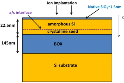
In the previous section it has been noticed that SPER needs a crystalline template in order to promote the crystallization during the thermal anneal. For this reason, implant conditions have to be chosen in order to obtain a partial amorphization of the silicon substrate and preserving a crystalline region on the bottom edge, so-called crystalline seed. In this study, SPER activation will be used for the dopant activation on FDSOI devices. The characteristic thickness of the access regions for this kind of device is approximately 22 nm. So, blanket SOI wafers, with a 22.5 nm thick silicon film over a 145 nm thick buried oxide, were used to a first study on SPER characteristics. The wafer configuration is shown in Figure 1.5. At the moment of implantation step, a thin native oxide layer of approximately 1.5 nm is present at silicon surface, due to the natural silicon oxidation.

A simple technique used to characterize the efficiency of the doping activation after thermal anneal is the four-point probe method. This technique allows to obtain an extremely reliable (measurement incertitude below 1%) measure of sheet resistance (RSHEET) value. Sheet resistance can be expressed

by: 400 500 600 700 800 900 1000 1100 1E18 1E19 1E20 1E21 M a x im u m c o n c e n tr a ti o n ( a t/ c m 3 ) Annealing temperature (°C) Phosphorus Arsenic Boron

(25)

23





j x sheet

dx

x

C

x

R

0

)

(

)

(

1 

(1.4)

Where C(x) is the active carrier concentration profile, µ(x) is the carrier mobility profile and xj is the

thickness of the implanted region. In this work, the thickness considered as xj is equal to the

amorphization depth after implantation. This choice rises from the fact that SPER mechanism leads to high dopants activation only in the amorphized region [Demenev 12], [Martinez-Limia 08]. This hypothesis neglects the active dopant presents in the crystalline seed.

Figure 1.5: Scheme of full sheet SOI sample used for SPER analysis.

Equation (1.1) contains both carrier concentration and mobility factors. These two parameters are correlated by the behavior reported in Figure 1.6 extracted by [Masetti 83]. However, once again, this behavior corresponds to condition of thermodynamic equilibrium. Since SPER is a non-equilibrium process, this behavior can be different. This point will be discussed in the following sections.

BOX Si substrate amorphous Si crystalline seed Ion Implantation 22.5nm 145nm a/c interface Native SiO₂~1.5nm x

(26)

24

Figure 1.6: Mobility-concentration behavior at thermodynamic equilibrium for boron, phosphorus and arsenic as a function of the concentration [Masetti 83].

1.2.1 n-type doping implantation and SPER activation: sheet resistance analysis

So far, only few papers in the literature [Woodard 06] have analyzed the junction optimization activated by SPER in terms of implantation conditions and sheet resistance results. In particular, no detailed studies describing the challenges and solutions for Fully Depleted Silicon On Insulator (FDSOI) access optimization are available at our knowledge. The low temperature junction optimization is not straightforward and is far from standard FDSOI high temperature process of reference (POR), as it will be discussed and highlighted in this section.

Samples described in Figure 1.5 have been implanted with different conditions and then annealed to activate the dopants by SPER. The different implantation and annealing conditions are listed in Table 1.1. In order to verify experimentally the thickness of the crystalline seed tseed predicted by KMC

simulations reported in Table 1, Transmission Electron Microscopy (TEM) measurement has been performed on the as-implanted sample 5 (S5). The TEM image in Figure 1.7 clearly shows a crystalline silicon seed with a thickness ranging from 3.5 to 5.5 nm. This thickness variation is due to the amorphous/crystalline (a/c) interface roughness. So, we can consider that tseed value extracted from

KMC simulation is correct within a range of ±2 nm. For both first (S1) and second (S2) samples, the doping conditions correspond to the ones used in the Process Of Reference (POR) for the state of the art FDSOI technology. It consists of four different implantations combining phosphorus and arsenic with a total dose of 5.5x1015_at/cm2_{. After the implantation, S1 has been subjected to spike annealing}

at 1050 °C (POR activated anneal) while S2 was treated with a low temperature anneal at 600 °C for 2 minutes.

1E19 1E20 1E21

0 20 40 60 80 100 120 140 160 180 200 220 240 M o b il it y (c m 2 /V x s ) Concentration (at/cm3) Boron Phosphorus Arsenic

(27)

25

Sample S1 S2 S3 S4 S5 S6 Annealing HT LT LT LT LT LT

Dopant As+P As+P As As P P

Dose (x1015_at/cm2₎ _5.5 _5.5 ₃ ₁ _1.7 ₁ tseed layer (nm) 5(*) 5 5 5 5 7

Table 1.1: Samples description with type of annealing, dopants implanted doses and crystalline seed thickness. (*)_{HT activation is not limited to the amorphized region.}

Figure 1.7: TEM image of Sample 5 after phosphorus high dose implantation.

Sheet resistance measurements have been performed on these six annealed samples and the results are reported in Figure 1.8. A significant degradation of 86% in sheet resistance is observed for S2 compared to S1. This clearly highlights that the process of reference implantation conditions that are optimized for the high temperature spike activation anneal (S1) are not adequate for low temperature SPER activation process (S2). In order to understand this effect, four different doping conditions (S3 to S6 in Table 1.1) have been tested. In samples S3 and S4, only arsenic implantations have been performed at different doses. Samples S5 and S6 have been implanted with phosphorus only, also varying the implantation dose. It was observed that reducing the total dose of dopants allows a great improvement of sheet resistance. Reducing the dose from 3×1015_at/cm3_{(S3) down to 1×10}15_at/cm3

(S4) leads to a 25% gain in sheet resistance. Similar improvement is observed in the sheet resistance value for phosphorus samples when implantation dose is reduced from 1.7×1015_at/cm3_{(S5) to 1×10}15

at/cm3_{(S6). This last sample shows significant improvement (18%) of sheet resistance value even}

compared to S1, where process of reference implant conditions and spike annealing have been used. Finally, comparing phosphorus (S6) and arsenic (S4) low dose samples, phosphorus appears to lead to an additional gain but at this stage additional analysis is needed, as will be detailed in sections 1.2.2 and 1.2.3.

To fairly compare the activation levels, it is first necessary to take into account the specificity of SPER activation at temperature below 600 °C, i.e. where dopants are efficiently activated only in the former amorphized region.

Resistivity is the key parameter that allows a better comparison of the activation level. In fact, it depends on the carrier concentration and mobility and is independent of the junction depth, as shown in equation (1.5):

(28)

26 𝜌(𝑥) = 1

𝐶(𝑥)µ(𝑥) (1.5)

The obtained results are reported in Figure 1.9, where similar trends to sheet resistance behavior (Figure 1.8) are observed. Strikingly, it has to be noted that sample implanted with low dose phosphorus and activated at low temperature by SPER (S6) outperforms even more clearly the resistivity of the process of reference sample (S1). On the other hand, S2 still exhibits a higher resistivity (+25%) compared to S1.

Figure 1.8: Sheet resistance measurements for samples described in Table 1.1.

Figure 1.9: Resistivity values for samples described in Table 1.1.

In order to understand the resistivity trend shown in Figure 1.9, Hall effect measurements results will be presented in the next section. This experimental procedure allows quantifying the active carriers dose and mobility. In the next section, the measured active dose will be compared with the total implanted dose for arsenic and phosphorus.

1.2.2 Determination of the optimum P and As concentration for LT SPER activation

The comparison between active dose obtained by Hall effect measurements and chemical dose extracted by KMC simulations shown in Figure 1.10 for arsenic implanted samples, enables to estimate the fraction of active dopants. In this figure, the dashed lines correspond to the total dopant dose present in the amorphized region, obtained by integrating the chemical dopant profile from the silicon surface to the amorphous/crystalline interface. The dopant profiles of arsenic samples are reported in Figure 1.11. The points of Figure 1.10 correspond to electron mobility and active dose values extracted by the Hall measurements. The arrow indicating the distance between the measured active dose and the total implanted dose, represents a phenomenon of clustering, i.e., the formation of inactive agglomeration that makes the dopants electrically inactive.

For the arsenic high dose sample (S3), the activated dopants fraction in the amorphized region corresponds to 35% of the total implanted dose (AsTOT,Dose). It is worth noticing that AsTOT,Dose for S3

obtained by this method is different from the value reported in Table 1.1 since a part of the implanted dose is trapped into the oxide present on the sample surface (as reported in Figure 1.7). Decreasing the implanted dose like in the case of S4, the activated dose fraction is estimated to be 96%. This value suggests that almost the total amount of arsenic implanted in the film has been efficiently activated by SPER. Thus, an optimal arsenic concentration that allows to full dopant activation can be extrapolated. Such value is found to be equal to 8x1020_at/cm3_{. This concentration can be defined as}

0 100 200 300 400 500 HT As+P LT As+P LT As high dos e LT As low dos e LT P high dos e LT P low dos e RSHEE T (Ω /□ ) +86% -18% 0E+0 1E-4 2E-4 3E-4 4E-4 5E-4 6E-4 7E-4 8E-4 9E-4 ρ (Ω xcm ) HT As +P LT As+P LT As high dos e LT As low dos e LT P h igh d os e LT P low dos e +25% -40%

(29)

27

clustering limit since for higher dopant concentrations, the implanted atoms start to form inactive aggregates, also named clusters. As evidenced by the active concentration measured on sample S3 (Figure 1.10), for concentrations well above the clustering limit, an overall reduction of the activation level appears. For arsenic, the most stable cluster form reported in literature [Skarlatos 07], [Pinacho 05] are the As2V, As3V, As4V i.e. aggregates of two, three or four atoms of arsenic and one vacancy. In

general, for concentrations higher than the clustering limit, arsenic has the tendency to aggregate with vacancies.

Figure 1.10: Dose and mobility measurements results for As samples. Total dose is reported as well for comparison.

Figure 1.11: Arsenic profiles after 2 minutes at 600°C annealing extracted by KMC simulation. Amorphous/crystalline (a/c) interface position is also reported.

Similar analysis is now performed for phosphorus. Phosphorus mobility versus carrier active dose measurements are displayed in Figure 1.12. The total dopant dose present in the amorphized region calculated integrating the dopant profiles illustrated in Figure 1.13 is reported as well. For the high dose phosphorus sample (S5), 80% of the total implanted dose in the amorphized region has been activated. Once again, this means that the activation is limited by dopant clustering. Decreasing the phosphorus implantation dose (S6) results in an almost complete activation (98%). Using KMC profiles presented in Figure 1.13, the clustering concentration limit is estimated around 6x1020 _at/cm3_.

Figure 1.12 shows that increasing the dose from quasi-ideal concentration (S6) to above clustering limit (S5) results in a dramatic mobility reduction. This affects directly the resistivity value (Figure 1.9), where ρS5 > ρS6. However, while the clustering concentration limit is already reached for low dose

sample (S6), a slightly higher activation is still observed for the higher dose (S5). In fact, the active dose increases from S6 to S5. This increase is explained by the fact that the amorphized depth in the S5 sample is thicker and that the concentration in this region is well below 6x1020 _at/cm3_{(see Figure 1.13).}

This deeper region of dopants with concentration below the clustering limit allows sample S5 to have an overall active dose higher than S6.

Clustering phenomenon As clustering limit 8x1020_at/cm3 S3 S4

(30)

28 Figure 1.12: Hall Mobility measurements results for P samples. Total dose is reported as well for comparison.

Figure 1.13: Phosphorus profiles after 2 minutes at 600°C annealing extracted by KMC simulation. Amorphous/crystalline (a/c) interface position is also reported.

Even though clustering limit for arsenic (8x1020_at/cm3_{) is higher than for phosphorus (6x10}20_at/cm3_),

better resistivity is shown for P implanted S6 (Figure 1.9). This can be explained by the mobility concentration curve at thermodynamic equilibrium [Masetti 84], where electron mobility for phosphorus is higher than for arsenic (see Figure 1.14). In addition, phosphorus is interesting for another aspect: since it has a smaller atomic mass compared to arsenic, it is possible to place a higher dose close to the BOX in a FDSOI access without full amorphization. This allows tuning a quasi-constant profile along the junction depth at concentration values close to the clustering limit extracted above. In Figure 1.14, it is also evidenced that the low dose As (S4) and P (S6) samples show an activation level very close from the thermodynamic equilibrium at 1050 °C.

Figure 1.14: Comparison between the electron mobility versus carrier concentration curves at 1050°C thermodynamic equilibrium [Masetti 84] and the experimental points at low dopant dose (S4 and S6). Carrier concentration of the experimental points is estimated using the measured active dose divided by the former amorphized region thickness.

Clustering phenomenon P clustering limit 6x1020_at/cm3 S5 S6

(31)

29

1.2.3 Dopant deactivation

Dopant activation by SPER drives the system to non-equilibrium state, so the application of a post annealing could lead to dopant deactivation phenomenon. Dopant deactivation arises from the high interstitial concentration left below the amorphous/crystalline interface after the implantation step. During subsequent thermal processing, these interstitials tend to interact to form bigger and more stable defects, the so–called end of range (EOR). They first form small interstitial clusters and further evolve towards {311} defects and dislocation loops. The presence of these defects generally has detrimental consequences for the device. During the activation process, EOR defects release interstitials that can interact with dopants in substitutional positions and cause deactivation. Similarly, vacancies can interact with active atoms and form electrically inactive clusters. Several study of deactivation phenomena are reported in literature especially for boron doping [Pawlak 04]

A post anneal of 30 minutes at 550 °C has been applied and the sheet resistance evolution of S1, S4 and S6 evaluated. However, in real device, the standard post activation anneal thermal budget, which is around 30 minutes at 400 °C, should provide even more stable activation. The aim of this section is to evaluate the evolution of sheet resistance values after post annealing for samples activated at high temperature and low temperature.

Figure 1.15: Sheet resistance – temperature curve for the in-situ experimental test of post annealing on S3.

Figure 1.16: Sheet resistance percentage variation after post annealing of 30 minutes at 550°C.

Sheet resistance measurements have been performed during the anneal. As an example, the complete post-annealing curve of sheet resistance as a function of the applied annealing temperature is shown for S3 in Figure 1.15. The point A corresponds to the sample just after dopant activation by SPER. A temperature ramp of 100 °C/min is then applied and the sheet resistance value increase, following the linear law R=R0(1+αT), up to point B. Then the sample is maintained for 30 minutes at constant

temperature of 550 °C. Sheet resistance increases until it reaches point C. The dopant deactivation phenomenon mainly occurs during this phase. Finally, the temperature is moved down to 25 °C reaching the point D. The sheet resistance variation between the point A and the point D represents

0 100 200 300 400 500 600 250 300 350 400 450 500 RS H E E T (  /s q .) Temperature (°C)

S3

As low dose A C B D Deactivation phenomenon 200 210 220 230 240 250 260 270 280 290 300 RS H E E T (  /s q .) S1 S4 S6

0 Post annealing time 30 min T=550°C