Entropic Optimal Transport between Unbalanced Gaussian Measures has a Closed Form

L’archive ouverte pluridisciplinaire HAL, est destinée au dépôt et à la diffusion de documents scientifiques de niveau recherche, publiés ou non, émanant des

The results of o-line calibration using [4] and the results of applying our self-calibration methods to eight stereo image pairs of the grid are compared in Table 1, for the left

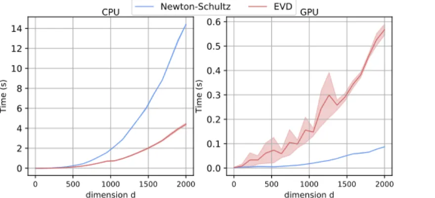
Although the proposed closed-form method is more computationally complex than block- level precoding schemes, our results show that in return, it provides substantial gains over

In this paper, we derive a closed- form expression of the WWB for 3D source localization using an arbitrary planar antenna array in the case of a deterministic known signal..

We observe that the con- ventional FRC curve reaches the closed-form FRC for some values of the sampling step of the discrete rendered image, as well as the parameters of the

Keywords: Credit Risk, Intensity Model, Strutural Model, Blak-Cox Model, Hybrid.. Model, Parisian options,

Observation of SEM pictures of the fluorine-altered substrates and comparison with bare Nitinol samples tend to confirm this erosive behavior: as well with

So for the simplex a different approach is needed and ours is based on the Laplace transform technique already used in our previous work in [6] for computing a certain class

References

[1] Agueh, M. and Carlier, G. (2011). Barycenters in the Wasserstein space. SIAM, 43(2):904–924. [2] Arjovsky, M., Chintala, S., and Bottou, L. (2017). Wasserstein generative adversarial networks. In Proceedings of the 34th International Conference on Machine Learning-Volume 70, pages 214–223.
[3] Benamou, J.-D. (2003). Numerical resolution of an “unbalanced” mass transport problem. ESAIM: Mathematical Modelling and Numerical Analysis - Modélisation Mathématique et Analyse Numérique, 37:851–868.
[4] Bhatia, R. (2007). Positive Definite Matrices. Princeton Series in Applied Mathematics. Princeton University Press, Princeton, NJ, USA.
[5] Bhatia, R., Jain, T., and Lim, Y. (2018). On the Bures-Wasserstein distance between positive definite matrices. Expositiones Mathematicae.
[6] Bojilov, R. and Galichon, A. (2016). Matching in closed-form: equilibrium, identification, and comparative statics. Economic Theory, 61(4):587–609.
[7] Bonneel, N., Rabin, J., Peyré, G., and Pfister, H. (2015). Sliced and Radon Wasserstein barycen-ters of measures. Journal of Mathematical Imaging and Vision, 51(1):22–45.
[8] Bures, D. (1969). An extension of Kakutani’s theorem on infinite product measures to the tensor product of semifinite w∗-algebras. Transactions of the American Mathematical Society, 135:199–212.
[9] Chen, Y., Georgiou, T. T., and Pavon, M. (2016). On the relation between optimal transport and Schrödinger bridges: A stochastic control viewpoint. Journal of Optimization Theory and Applications, 169(2):671–691.
[10] Chen, Y., Georgiou, T. T., and Pavon, M. (2016). Optimal steering of a linear stochastic system to a final probability distribution, part i. IEEE Transactions on Automatic Control, 61(5):1158–1169. [11] Chen, Y., Georgiou, T. T., and Pavon, M. (2018). Optimal steering of a linear stochastic system to a final probability distribution—part iii. IEEE Transactions on Automatic Control, 63(9):3112–3118.
[12] Chen, Y., Georgiou, T. T., and Tannenbaum, A. (2018). Optimal transport for Gaussian mixture models. IEEE Access, 7:6269–6278.
[13] Chizat, L., Peyré, G., Schmitzer, B., and Vialard, F.-X. (2018a). An interpolating distance between optimal transport and Fisher–Rao metrics. Foundations of Computational Mathematics, 18(1):1–44.
[14] Chizat, L., Peyré, G., Schmitzer, B., and Vialard, F.-X. (2018b). Scaling algorithms for unbalanced optimal transport problems. Mathematics of Computation, 87(314):2563–2609. [15] Cuturi, M. (2013). Sinkhorn distances: Lightspeed computation of optimal transport. In
Advances in Neural Information Processing Systems, pages 2292–2300.
[16] Cuturi, M. and Peyré, G. (2016). A smoothed dual approach for variational Wasserstein problems. SIAM Journal on Imaging Sciences, 9(1):320–343.
[17] del Barrio, E. and Loubes, J.-M. (2020). The statistical effect of entropic regularization in optimal transportation. arxiv preprint arXiv:2006.05199.
[18] Dereich, S., Scheutzow, M., and Schottstedt, R. (2013). Constructive quantization: Approxima-tion by empirical measures. In Annales de l’Institut Henri Poincaré, Probabilités et Statistiques, volume 49, pages 1183–1203.
(12)
[19] Dowson, D. and Landau, B. (1982). The Fréchet distance between multivariate normal distribu-tions. Journal of Multivariate Analysis, 12(3):450 – 455.
[20] Feydy, J., Séjourné, T., Vialard, F., Amari, S., Trouvé, A., and Peyré, G. (2019). Interpolating between optimal transport and MMD using Sinkhorn divergences. In The 22nd International Conference on Artificial Intelligence and Statistics, AISTATS 2019, 16-18 April 2019, Naha, Okinawa, Japan, pages 2681–2690.
[21] Figalli, A. (2017). The Monge–Ampère equation and its applications.
[22] Fournier, N. and Guillin, A. (2015). On the rate of convergence in Wasserstein distance of the empirical measure. Probability Theory and Related Fields, 162(3-4):707–738.
[23] Frogner, C., Zhang, C., Mobahi, H., Araya, M., and Poggio, T. A. (2015). Learning with a Wasserstein loss. In Advances in Neural Information Processing Systems, pages 2053–2061. [24] Gelbrich, M. (1990). On a formula for the l2 Wasserstein metric between measures on Euclidean
and Hilbert spaces. Mathematische Nachrichten, 147(1):185–203.
[25] Genevay, A., Chizat, L., Bach, F., Cuturi, M., and Peyré, G. (2019). Sample complexity of sinkhorn divergences. In Chaudhuri, K. and Sugiyama, M., editors, Proceedings of Machine Learning Research, volume 89 of Proceedings of Machine Learning Research, pages 1574–1583. PMLR.
[26] Genevay, A., Cuturi, M., Peyré, G., and Bach, F. (2016). Stochastic optimization for large-scale optimal transport. In Advances in Neural Information Processing Systems, pages 3440–3448. [27] Genevay, A., Peyre, G., and Cuturi, M. (2018). Learning generative models with Sinkhorn
divergences. In Storkey, A. and Perez-Cruz, F., editors, Proceedings of the Twenty-First Interna-tional Conference on Artificial Intelligence and Statistics, volume 84 of Proceedings of Machine Learning Research, pages 1608–1617, Playa Blanca, Lanzarote, Canary Islands. PMLR. [28] Gerolin, A., Grossi, J., and Gori-Giorgi, P. (2020). Kinetic correlation functionals from the
entropic regularization of the strictly correlated electrons problem. Journal of Chemical Theory and Computation, 16(1):488–498.
[29] Heusel, M., Ramsauer, H., Unterthiner, T., Nessler, B., and Hochreiter, S. (2017). Gans trained by a two time-scale update rule converge to a local Nash equilibrium. In Advances in neural information processing systems, pages 6626–6637.
[30] Higham, N. J. (2008). Functions of Matrices: Theory and Computation (Other Titles in Applied Mathematics). Society for Industrial and Applied Mathematics, USA.
[31] Janati, H., Cuturi, M., and Gramfort, A. (2020). Debiased sinkhorn barycenters. In Proceedings of the 34th International Conference on Machine Learning.
[32] Kolouri, S., Nadjahi, K., Simsekli, U., Badeau, R., and Rohde, G. (2019). Generalized sliced wasserstein distances. In Advances in Neural Information Processing Systems, pages 261–272. [33] Liero, M., Mielke, A., and Savaré, G. (2016). Optimal transport in competition with reaction:
the Hellinger–Kantorovich distance and geodesic curves. SIAM Journal on Mathematical Analysis, 48(4):2869–2911.
[34] Liero, M., Mielke, A., and Savaré, G. (2018). Optimal entropy-transport problems and a new Hellinger–Kantorovich distance between positive measures. Inventiones Mathematicae, 211(3):969–1117.
[35] Luise, G., Salzo, S., Pontil, M., and Ciliberto, C. (2019). Sinkhorn barycenters with free support via frank-wolfe algorithm. In Advances in Neural Information Processing Systems.
[36] Malagò, L., Montrucchio, L., and Pistone, G. (2018). Wasserstein riemannian geometry of positive definite matrices. arXiv preprint arXiv:1801.09269.
[37] Mallasto, A., Gerolin, A., and Minh, H. Q. (2020). Entropy-regularized 2-wasserstein distance between gaussian measures. Arxiv preprint arXiv:2006.03416.
[38] Mena, G. and Niles-Weed, J. (2019). Statistical bounds for entropic optimal transport: sample complexity and the central limit theorem. In Advances in Neural Information Processing Systems 32, pages 4541–4551. Curran Associates, Inc.
[39] Muzellec, B. and Cuturi, M. (2018). Generalizing point embeddings using the wasserstein space of elliptical distributions. In Advances in Neural Information Processing Systems 31, pages 10237–10248. Curran Associates, Inc.
(13)
[40] Paty, F.-P. and Cuturi, M. (2019). Subspace robust wasserstein distances. In International Conference on Machine Learning, pages 5072–5081.
[41] Peyré, G. and Cuturi, M. (2019). Computational optimal transport. Foundations and Trends R
in Machine Learning, 11(5-6):355–206.
[42] Rabin, J., Peyré, G., Delon, J., and Bernot, M. (2011). Wasserstein barycenter and its application to texture mixing. In International Conference on Scale Space and Variational Methods in Computer Vision, pages 435–446. Springer.
[43] Ramdas, A., Trillos, N. G., and Cuturi, M. (2017). On wasserstein two-sample testing and related families of nonparametric tests. Entropy, 19(2):47.
[44] Santambrogio, F. (2015). Optimal transport for applied mathematicians. Birkhauser.
[45] Séjourné, T., Feydy, J., Vialard, F.-X., Trouvé, A., and Peyré, G. (2019). Sinkhorn divergences for unbalanced optimal transport. arXiv preprint arXiv:1910.12958.
[46] Shirdhonkar, S. and Jacobs, D. W. (2008). Approximate earth mover’s distance in linear time. In IEEE Conference on Computer Vision and Pattern Recognition, pages 1–8. IEEE.
[47] Takatsu, A. (2011). Wasserstein geometry of Gaussian measures. Osaka J. Math., 48(4):1005– 1026.
[48] Titouan, V., Flamary, R., Courty, N., Tavenard, R., and Chapel, L. (2019). Sliced gromov-wasserstein. In Advances in Neural Information Processing Systems, pages 14726–14736. [49] Villani, C. (2009). Optimal Transport: Old and New, volume 338. Springer Verlag.
(14)
Appendix
5.1 The Newton-Schulz algorithm
Algorithm 1 NS Monge Iterations Input: PSD matrix A, B,  > 0
Y ← (1+)kBkB , Z ← (1+)kAkA while not converged do
T ← (3I − ZY)/2 Y ← YT Z ← TZ end while Y ← q kBk kAkY, Z ← q kAk kBkZ Output: Y = TAB, Z = TBA
The main bottleneck in computing TABis that of
com-puting matrix square roots. This can be performed using singular value decomposition (SVD) or, as suggested in [39], using Newton-Schulz (NS) iterations [30, §5.3]. In particular, Newton-Schulz iterations have the advantage of yielding both roots, and inverse roots. Hence, to compute TAB, one would run NS a first time to obtain A12 and
A−
1
2, and a second time to get (A
1 2BA 1 2) 1 2.
In fact, as a direct application of [30, Theorem 5.2], one can even compute both TABand TBA= TAB−1
in a single run by initializing the Newton-Schulz algorithm
with A and B, as in Algorithm 1. Using (6), and noting that B2(A, B) = TrA+TrB−2Tr(TABA), this implies that a single run of NS is sufficient to compute B2(A, B), ∇
AB2(A, B) and
∇BB2(A, B) using basic matrix operations. The main advantage of Newton-Schultz over SVD is
that it its efficient scalability on GPUs, as illustrated in Figure 4.
Newton-Schulz iterations are quadratically convergent under the condition k Id − (A 0 0 B)
2
k < 1, as shown in [30, Theorem 5.8]. To meet this condition, it is sufficient to rescale A and B so that their norms equal (1 + ε)−1 for some ε > 0, as in the first step of Algorithm 1 (which can be skipped if kAk < 1 (resp. kBk < 1)). Finally, the output of the iterations are scaled back, using the homogeneity (resp. inverse homogoneity) of eq. (5) w.r.t. A (resp. B).
A rough theoretical analysis shows that both Newton-Schulz and SVD have a O(d3) complexity in
the dimension. Figure 4 compares the running times of Newton-Schulz iterations and SVD on CPU or GPU used to compute both A
2 and A− 1
2. We simulate a batch of positive definite matrices A
following the Wishart distribution W (Idd, d) to which we add 0.1 Id to avoid numerical issues when
computing inverse square roots. We display the average run-time of 50 different trials along with its ± std interval. Notice the different magnitudes between CPUs and GPUs. As a termination criterion, we first run EVD to obtain A
1 2
evd and A −12
evd and stop the Newton-Schultz algorithm when its n-th
running estimate A 1 2 n verifies: kA 1 2 n − A 1 2 evdk1 ≤ 10
−4. Notice the different order of magnitude
between CPUs and GPUs. Moreover, the computational advantage of Newton-Schultz on GPUs can be further increased when computing multiple square roots in parallel.
0 500 1000 1500 2000 dimension d 0 2 4 6 8 10 12 14 Time (s) CPU 0 500 1000 1500 2000 dimension d 0.0 0.1 0.2 0.3 0.4 0.5 0.6 Time (s) GPU Newton-Schultz EVD
(15)
2= 0.01 2= 0.1 2= 0.5 2= 1.0 2= 10
Figure 5: Effect of regularization on transportation plans. When σ goes to 0 (left), the transportation plan concentrates on the graph of the linear Monge map. When σ goes to infinity (right), the transportation plan converges to the independent coupling.
5.2 Effects of regularization strength.
We provide numerical experiments to illustrate the behaviour of transportation plans and corre-sponding distances as σ goes to 0 or to infinity. As can be seen from eq. (14), when σ → 0 we recover the Wasserstein-Bures distance (3), and the optimal transportation plan converges to the Monge map (5). When on the contrary σ → ∞, Sinkhorn divergences Sε(α, β)
def
= OTε(α, β) − 1
2(OTε(α, α) + OTε(β, β)) convergence to MMD with a −c kernel (where c is the optimal transport
ground cost) [27]. With a −`2kernel, MMD is degenerate and equals 0 for centered measures.
0.50 0.25 0.00 0.25 0.50
Bures geodesic
Sinkhorn-Bures geodesic, = 1.0
4 3 2 1 0 1 2 3 4 0.50 0.25 0.00 0.25 0.50
Euclidean geodesic
Figure 7: Bures, Sinkhorn-Bures, and Euclidean geodesics. Sinkhorn-Bures trajectories converge to Bures geodesics as σ goes to 0, and to Euclidean geodesics as σ goes to infinity.
(16)
0.00 0.05 0.10 0.15 0.20 0.25 d = 2 0.0 0.2 0.4 0.6 0.8 d = 5 10−2 10−1 100 101 102 σ 0.0 0.5 1.0 1.5 2.0 2.5 d = 10 Bures Bures-Sinkhorn
Figure 6: Numerical convergence of B2σ(A, B) −12(B 2
σ(A, A) + B2σ(B, B)) to B2(A, B) as σ
goes to 0 and to 0 as σ goes to infinity.
5.3 Proofs of technical results
We provide in this appendix the proofs of the results in the paper, as well as some technical lemmas used in solving Sinkhorn’s equations in closed form.
Proof of Lemma 1.
Proof. Let d ¯α(x) = dα(x + a) (resp. d ¯β(y) = dβ(y + b), d¯π(x, y) = dπ(x + a, y + b), such that ¯
α, ¯β and ¯π are centered. Then, ∀π ∈ Π(α, β), (i) ¯π ∈ Π( ¯α, ¯β), (ii) KL(πkα ⊗ β) = KL(¯πk ¯α ⊗ ¯β) (iii) R Rd×Rdkx − yk 2π(x, y) =R Rd×Rdk(x − a) − (y − b)k 2dπ(x, y) = ka − bk2+R Rd×Rdkx − yk2dπ(x, y)
(17)
Proof of Proposition 1.
Proof. The exponent inside the integral can be written as: e −kx−yk2 2σ2 +h(y)dα(y) ∝ e −kx−yk2 2σ2 −12(y >Xy−y>A−1y) dy ∝ e−12(y >(Id σ2+X+A −1)y)+x> y σ2 dy
which is integrable if and only if X + A−1+ 1
σ2Id  0. Moreover, up to a multiplicative factor,
the exponentiated Sinkhorn transform is equivalent to a Gaussian convolution of an exponentiated quadratic form. Lemma 4 applies:
e−Tα(h)= Z Rd e −kx−yk2 2σ2 +f (y)dα(y) ∝ Z Rd e −kx−yk2 2σ2 +Q(X)(y)+Q(A −1)(y) dy ∝ exp Q Id σ2 ? exp Q(X) + Q(A −1) ∝ exp Q Id σ2 ? exp Q(X + A −1) ∝ exp Q((Id +σ2X + σ2A−1)−1(X + A−1)) . ∝ exp  Q( 1 σ2X 0−1(X0− Id)). ∝ exp  Q( 1 σ2(Id −X 0−1)).
Therefore Tα(h) is up to an additive constant given by Q(σ12(X0−1− Id)).
Finally, since B and X0 are positive definite, the positivity condition of Y0holds and Tβ can be
applied again to get Tβ(Tα(h)).
Proof of Proposition 2.
Proof. Let U0 = V0 = 0. Applying Proposition 1 to the initial pair of potentials Q(U0), Q(V0)
leads to the sequence of quadratic Sinkhorn potentials fn2 = Q(Un) and gn2 = Q(Vn) where:
Vn+1= 1 σ2((σ 2 Un+ σ2A−1+ Id)−1− Id) Un+1= 1 σ2((σ 2V n+1+ σ2B−1+ Id)−1− Id).
The change of variable:
Fn= σ2Un+ σ2A−1+ Id
Gn= σ2Vn+ σ2B−1+ Id
leads to (17).
We turn to show that this algorithm converges. First, note that since F0, G0∈ S++d , a straightforward
induction shows that ∀n ≥ 0, Fn, Gn ∈ S++d . Next, let us write the decoupled iteration on F:
F ← σ2A−1+ (σ2B−1+ F−1)−1 (42)
Let ∀X ∈ S++d , φ(X)def= σ2A−1+ (σ2B−1+ X−1)−1 ∈ Sd
++. The first differential of φ admits
the following expression: ∀X ∈ Sd
++, ∀H ∈ R
d×d, Dφ(X)[H] = (Id +σ2XB−1)−1H(σ2B−1X + Id)−1. (43)
Hence, kDφ(X)[H]kop ≤ k(Id +σ2XB−1)−1k2opkHkop. Plugging H = Id, we get that
kDφ(X)kop = k(Id +σ2XB−1)−1k2op. Finally, by matrix similarity
k(Id +σ2XB−1)−1k op= k(Id +σ2B− 1 2XB− 1 2)−1kop< 1 ,
(18)
which implies that kDφ(X)kop < 1 for X ∈ S++d and σ2> 0. The same arguments hold for the
iterates (Gn)n≥0.
From (42) and using Weyl’s inequality, we can bound the smallest eigenvalue of Fnfrom under:
∀n, λd(Fn) ≥ σ 2
λ1(A) (where λd(F) is the smallest eigenvalue of F and λ1(A) is the biggest
eigenvalue of A). Hence, the iterates live in Adef= Sd
++∩ {X : λd(X) ≥ σ 2
λ1(A)}. Finally, for all
X ∈ A, k(Id +σ2B−12XB−12)−1k op= 1 λd(Id +σ2B−1/2XB−1/2) = 1 1 + σ2λ d(B−1/2XB−1/2) ≤ 1 1 + σ2λ d(B−1)λd(X) ≤ 1 1 +λ σ4 1(B)λ1(A)
Which proves the uniform bound
Proof of Proposition 3.
Proof. Combining the two equations in (20) yields G = σ2B−1+ (G−1+ σ2A−1)−1
⇔ GA−1 = σ2B−1A−1+ (AG−1+ σ2Id)−1
⇔ C−1= σ2(AB)−1+ (C + σ2Id)−1
⇔ C−1(C + σ2Id) = σ2(AB)−1(C + σ2Id) + Id ⇔ Id +σ2C−1= σ2(AB)−1(C + σ2Id) + Id
⇔ C + σ2Id = σ2(AB)−1(C + σ2Id)C + C
⇔ C2+ σ2C − AB = 0. (44)
Given that A and G−1 are positive, their product C = AG−1 can be written: AG−1 = A12(A12G−1A12)A−12, thus AG−1is similar to the positive matrix A
2G−1A12. Therefore, one
can write an eigenvalue decomposition of C = PΣP−1with a positive diagonal matrix Σ. Substitut-ing in (21), it follows that C and AB share the same eigenvectors with modified eigenvalues. Thus, it is sufficient to find the real roots of the polynomial x 7→ x2+ σ2
x − ab with a, b ∈ R++which
are given by: x1= −σ 2 2 − q ab +σ4 4 and x2= − σ2 2 + q ab +σ4
4. Since C is the product of the
positive definite matrices G−1and A, its eigenvalues are all positive. Discarding the negative root, the closed form follows immediately.
Indeed, by direct calculation, computing the square of the solution C leads to the equation (21):
C2= AB +σ 4 2 Id −σ 2  AB +σ 4 4 Id  1 2 = AB − σ2C. The second equality is obtained by observing that
(A 1 2(A 1 2BA 1 2 +σ4 4 Id) 1 2A− 1 2)2= A 1 2(A 1 2BA 1 2 +σ4 4 Id)A −12 = AB +σ4 4 Id, i.e. that  AB +σ44Id 1 2 = A12(A12BA12+σ44Id)12A−12.
(19)
Proof of Lemma 2
Proof. It follows from elementary properties of Gaussian measures that the first and second marginals of π are respectively α and β. Hence,
Z Rd×Rd kx − yk2dπ(x, y) = Z Rd×Rd kxk2dπ(x, y) + Z Rd×Rd kyk2dπ(x, y) − 2 Z Rd×Rd hx, yidπ(x, y) (45) = Z Rd kxk2dα(x) + Z Rd kyk2dβ(y) − 2 Z Rd×Rd hx, yidπ(x, y) (46) = Tr(A) + Tr(B) − 2Tr(C). (47)
Next, using the closed form expression of the Kullback-Leibler divergence between Gaussian mea-sures, KL (πkα ⊗ β) = 12Trh(A 0 0 B) −1 A C CT B i − 2n + log det (A 0 0 B) − log det A C CT B  (48) = 12 log det A + log det B − log det CA CT B . (49)
Optimal transport plan and OTσ
dπ dxdy(x, y) = exp  f (x) + g(y) − kx − yk2 2σ2  dα dx(x) dβ dy(y) ∝ exp  Q(A−1)(x) +f (x) + g(y) − kx − yk 2 2σ2 + Q(B −1)(y)  ∝ exp  Q(U + A−1)(x) + Q(V + B−1)(y) + Q( σ2Id − Id σ2 −Id σ2 Id σ2 )(x, y)  = exp  Q(U+A−1 0 0 V+B−1)(x, y) + Q( Id σ2 − Id σ2 −Id σ2 Id σ2 )(x, y)  = exp  Q( Id σ2+U+A −1 Id σ2 −Id σ2 Id σ2+V+B −1)(x, y)  = exp  Q( F σ2 − Id σ2 −Id σ2 G σ2 )(x, y)  = exp (Q(Γ)(x, y)) with Γdef=  F σ2 − Id σ2 −Id σ2 G σ2
. Moreover, since G2  0 , and its Schur complement satisfies F σ2 − 1
σ2G
−1 = A−1  0, we have that Γ  0. Therefore π is a Gaussian N (H) with the covariance
matrix given by the block inverse formula:
H = Γ−1 (50) = σ2(F − G −1)−1 (GF − Id)−1 (FG − Id)−1 (G − F−1)−1  (51) = A C C> B  , (52)
where we used the optimality equations (20) and the definition of C = AG−1.
We can now conclude the proof of Theorem 1 by computing OTσ(α, β) using Lemma 2. Let
R = A12BA 1
2. Using the closed form expression of C in (22), it first holds that
Zdef= A−12CA 1 2 = (R +σ 4 4 Id) 1 2 σ2 2 Id . (53)
(20)
Moreover, since R = R>, it holds that Z = Z>. Hence,
det CA CT B = det(A) det(B − C>A−1C)
= det(A12BA 1 2 − A 1 2C>A−1CA 1 2) = det(R − Z>Z) = det(R − Z2) = det(σ2(R +σ 4 4 Id) 1 2 −σ 4 2 Id) = (σ 2 2 ) ddet((4R + σ4Id)1 2 − σ2Id). (54)
Since the matrices inside the determinant commute, we can use the identity P − Q = (P2− Q2)(P +
Q)−1to get rid of the negative sign. Equation (54) then becomes: (σ 2 2 ) ddet((4R + σ4Id)1 2 − σ2Id) = (σ 2 2 )
ddet(4R) det((4R + σ4Id)1
2 + σ2Id)−1
= (2σ2)ddet(AB) det((4R + σ4Id)12 + σ2Id)−1
. Plugging this expression in (25), the determinant of A and B cancel out and we finally get:
B2σ(A, B) = Tr(A) + Tr(B) − Tr(4A12BA 1
2 + σ4Id) 1
2+ dσ2−
σ2d log(2σ2) + σ2log det(4A12BA 1 2 + σ4Id) 1 2 + σ2Id  . Proof of Proposition 4
Proof. Using Lemma 2, eq. (7) becomes B2σ(A, B) = min C: A C CT B  ≥0 n
Tr(A) + Tr(B) − 2Tr(C) + σ2(log det A + log det B − log det CA CT B)
o , which gives eq. (26). Let us now prove eq. (27). A necessary and sufficient condition for CA CT B ≥ 0
is that there exists a contraction K (i.e. K ∈ Rd : kKkop ≤ 1) such that C = A 1 2KB
2 [4, Ch. 1].1
With this parameterization, we have (using Schur complements) that det CA CT B = det B det(A − CB
−1C>)
= det B det A det(Id −KK>)
Hence, injecting this in Equation (26), we have the following equivalent problem: B2σ(A, B) = min K∈Rd×d:kKk op≤1 TrA + TrB − 2TrA 1 2KB 1 2 − σ2ln det(Id −KK>) (55)
Let’s prove that both problems are convex. • (26): The set {C : A C CT B  ≥ 0} is convex, since A C1 CT1 B  ≥ 0 and  A C2 CT2 B  ≥ 0 implies that A (1−θ)C1+θC2 (1−θ)CT 1+θCT2 B  = (1 − θ)CA C1T 1 B  + θCA C2T 2 B  ≥ 0. Following the same decomposition, the concavity of the log det function implies that C → log det A C
CT B is concave, and hence that the objective function of (26) is convex.
• (27): The ball Bop def
= {K ∈ Rd×d: kKkop ≤ 1} is obviously convex. Hence, there remains
to prove that f (K) : K ∈ Bop → log det(Id −KK>) is concave. Indeed, it holds that
f (K) = log det KId KT Id. Hence, ∀K, H ∈ Bop, ∀t ∈ [0, 1],
f ((1 − t)K + tH) = log det(1 − t) Id K KT Id + t Id H HT Id  ≥ (1 − t) log det Id K KT Id + t log det Id H HT Id  = (1 − t)f (K) + tf (H), where the second line follows from the concavity of log det.
(21)
Proof of Proposition 5
Proof. By Proposition 4, (26) is convex, hence strong duality holds. Ignoring the terms not depending on C, problem (26) can be written using the redundant parameterization X = X1X3X2X4:
D(A, B)def= min
X0 X1=A,X4=B − Tr(X2) − Tr(X3) − σ2log det (X) (56) = min X0 X1=A,X4=B − hX, 0 Id Id 0i − σ 2log det (X) (57) = min X0 X1=A,X4=B F (X), (58)
where the functional F is convex. Moreover, its Legendre transform is given by: F?(Y) = max X0hX, Y + 0 Id Id 0i + σ 2 log det (X) = −σ2log det)? Y + 0 Id Id 0  = σ2(− log det)? 1 σ2 Y + 0 Id Id 0   = −σ2log det  − 1 σ2 Y + 0 Id Id 0   − 2σ2d = −σ2log det − Y + 0 Id Id 0 − 2d(σ 2− σ2log(σ2)).
Let H be the linear operator H : X 7→ (X1, X4). Its conjugate operator is defined on S++d × S d ++
and is given by H?(F, G) = (F 0
0 G). Therefore, Fenchel’s duality theorem leads to:
D(A, B) = max F,G0− hF, Ai − hG, Bi − F ?(−H?(F, G)) = max F,G0− hF, Ai − hG, Bi + σ 2log det F − Id − Id G  + 2d(σ 2− σ2log(σ2)) = max F,G0− hF, Ai − hG, Bi + σ
2log det (FG − Id) + 2d(σ2
− σ2log(σ2))
Where the last equality follows from the fact that Id and G commute. Therefore, reinserting the discarded trace terms, the dual problem of (26) can be written as
max
F,G0
n
− hF, Ai − hG, Bi + σ2log det (FG − Id)
+ Tr(A) + Tr(B) + σ2log det AB + 2dσ2(1 − log σ2))o. (59)
Proof of Proposition 6
Proof. (i) Optimality: Canceling out the gradients in eq. (28) leads to the following optimality conditions: −A + σ2G(FG − Id)−1 = 0 −B + σ2(FG − Id)−1F = 0, (60) i.e. F = σ2A−1+ G−1 G = σ2B−1+ F−1 (61)
(22)
(ii) Differentiabilty: Using Danskin’s theorem on problem (28) leads to the formula of the gradient as a function of the optimal dual pair (F, G). Indeed, keeping in mind that ∇Alog det(A) = −A−1
and using the change of variable of Proposition 2, we recover the dual potentials of Corollary 1: ∇Bσ2(A, B) = Id −F∗+ σ2A−1, Id −G∗+ σ2B−1
= −σ2(U, V) Using Corollary 1, it holds that
∇ABσ2(A, B) = −σ2U = Id −B(C + σ2Id)−1 = Id −B  (AB +σ 4 4 Id) 1 2 +σ 2 2 Id −1 = Id −B 1 2  (B 1 2AB 1 2 +σ 4 4 Id) 1 2 +σ 2 2 Id −1 B 1 2 = Id −B12  D12 +σ 2 2 Id −1 B12, where Ddef= B12AB12 +σ4 4 Id.
(iii) Convexity: Assume without loss of generality that B is fixed and let G : B 7→ ∇ABσ2(A, B).
As long as σ > 0, G is differentiable as a composition of differentiable functions. Let’s show that the Hessian of ψ : A 7→ Bσ2(A, B) is a positive quadratic form. Take a direction H ∈ S+d. It holds:
∇2
ABσ2(A, B)(H, H) = hH, JacG(A)(H)i
= Tr(H JacG(A)(H)).
For the sake of clarity, let’s write G(A) = Id −L(W (φ(A))) with the following intermediary functions: L : A 7→ B12AB12 Q : A 7→ A12 φ : A 7→ Q(L(A) +σ 4 4 Id) W : A 7→ (A +σ 2 2 Id) −1.
Moreover, their derivatives are given by: JacL(A)(H) = B
1 2HB12
JacW(A)(H) = −(A +
σ2 2 Id) −1H(A +σ2 2 Id) −1 JacQ(A)(H) = Z,
where Z ∈ S+d is the unique solution of the Sylvester equation: ZA 1
2 + A12Z = H.
Using the chain rule:
JacG(A)(H) = − JacL(W (φ(A)))(JacW(φ(A))(Jacφ(A)(H)))
= −B
2JacW(φ(A))(Jacφ(A)(H))B 1 2 = B 1 2  φ(A) + σ 2 2 Id −1 Jacφ(A)(H)  φ(A) + σ 2 2 Id −1 B 1 2 = B12  D12 +σ 2 2 Id −1 Jacφ(A)(H)  D12 +σ 2 2 Id −1 B12.
(23)
Again using the chain rule:
Ydef= Jacφ(A)(H) = JacQ(L(A) +
σ4 4 Id)((JacL(A))(H)) = JacQ(L(A) + σ4 4 Id)(B 1 2HB 1 2) = JacQ(D)(B 1 2HB12). Therefore, Y  0 is the unique solution of the Sylvester equation:
YD12 + D12Y = B12HB12. Combining everything:
= Tr (H JacG(A)(H)) = Tr HB 1 2  D 1 2+σ 2 2 Id −1 Y  D 1 2 +σ 2 2 Id −1 B 1 2 ! = Tr B12HB12  D12 +σ 2 2 Id −1 Y  D12 +σ 2 2 Id −1! .
Since H and Y are positive, the matrices B12HB12and  D12 +σ22Id −1 Y  D12 +σ22Id −1 are positive semi-definite as well. Their product is similar to a positive semi-definite matrix, therefore the trace above is non-negative.
Given that A and H are arbitrary positive semi-definite matrices, it holds that ∇2
ABσ2(A, B)(H, H) ≥ 0
Therefore, A 7→ Bσ2(A, B) is convex.
Counter-example of joint convexity: If Bσ2 were jointly convex , then δ def
= : A → Bσ2(A, A)
would be a convex function.
In the 1-dimensional case with σ = 1, one can see that this would be equivalent to x → ln((x2+ 1)12 + 1) − (x2+ 1)12 being convex, whereas it is in fact strictly concave.
(iv) Minimizer ofφBWith fixed B, cancelling the gradient of φB def
= : A 7→ Bσ2(A, B) leads to
A = B − σ2Id which is well defined if and only if B  σ2Id. However, if B − σ2Id is not positive
semi-definite, write the eigenvalue decomposition: B = PΣP>and define A0 def
= P(Σ−σ2Id) +P>
where the operator x+= max(x, 0) is applied element-wise. Then:
∇AφB(A0) = Id −PΣ 1 2P>  (P(Σ2− σ2Σ) +P>+ σ4 4 Id) 1 2 +σ 2 2 Id −1 PΣ12P> = Id −PΣ 1 2  ((Σ2− σ2Σ)++ σ4 4 Id) 1 2+σ 2 2 Id −1 Σ 1 2P> = Id −PΣ12 (Σ − σ2Id)++ σ2Id −1 Σ12P> = P(Id −Σ 1 2 (Σ − σ2Id)++ σ2Id−1Σ 1 2)P> = 1 σ2P(σ 2Id −Σ) +P>
Thus, given that (Σ − σ2Id)
+(σ2Id −Σ)+ = 0, it holds, for any H ∈ S+d:
hH − A0, ∇AφB(A0)i = hP>HP − (Σ − σ2Id)+, (σ2Id −Σ)+i
= hP>HP, (σ2Id −Σ)+i
= Tr(P>HP(σ2Id −Σ)+) ≥ 0
Where the last inequality holds since both matrices are positive semi-definite. Given that φBis
(24)
Proof of Theorem 2
Proof. This theorem is a generalization of [31, Thm 3] for multivariate Gaussians. First we are going to break it down using the centering lemma 1. For any probability measure µ, let ¯µ denote its centered transformation. The debiased barycenter problem is equivalent to:
min β∈G K X k=1 wkSσ(αk, β) = min β∈G K X k=1 wkOTσ(αk, β) − 1 2(OTσ(αk, αk) + OTσ(β, β)) = min β∈G K X k=1 wkkak− Eβ(X)k2+ wkOTσ( ¯αk, ¯β) − 1 2(wkOTσ( ¯αk, ¯αk) + OTσ( ¯β, ¯β)) = min b∈Rd β∈G,Eβ(X)=0 K X k=1 wkkak− bk2+ wkOTσ( ¯αk, β) − 1 2(wkOTσ( ¯αk, ¯αk) + OTσ(β, β)) (62)
Therefore, since both arguments are independent, we can first minimize over b to obtain Eβ(X) =
b =PK
k=1wkak. Without loss of generality, we assume from now on that ak= 0 for all k.
The rest of this proof is adapted from [31], Thm 3 to d ≥ 1. Janati et al. [31] showed that Sσ is
differentiable and convex (w.r.t. one measure at a time) on sub-Gaussian measures where the notion of differentiability is different from the usual Fréchet differentiability: a function F : G → R is differentiable at α if there exists ∇F (α) ∈ C(Rd) such that for any displacement tδα with t > 0 and δα = α1− α2with α1, α2∈ G, and
F (α + tδα) = F (α) + thδα, ∇F (α)i + o(t) , (63) where hδα, ∇F (α)i =R
Rd∇F (α)dδα.
Moreover, F is convex if and only if for any α, α0∈ G:
F (α) ≥ F (α0) + hα − α0, ∇F (α0)i , (64) Let (fk, gk) denote the potentials associated with OTσ(αk, β) and hβthe autocorrelation potential
associated with OTσ(β, β). If β is sub-Gaussian, it holds: ∇βSσ(αk, β) = gk− h. Therefore, from
(64) a probability measure β is the debiased barycenter if and only if for any direction µ ∈ G, the optimality condition holds:
h K X k=1 wk∇βSσ(αk, β), µ − βi ≥ 0 ⇔ K X k=1 wkhgk− hβ, µ − βi ≥ 0 (65)
Moreover, the potentials (fk), (gk) and h must verify the Sinkhorn optimality conditions (10) for all
k and for all x β-a.s and y α-a.s:          e fk(x) 2σ2  R Rde −kx−yk2+gk(y) 2σ2 dβ(y)  = 1, e gk(x) 2σ2  R Rde −kx−yk2+fk(y) 2σ2 k(y)  = 1. e h(x) 2σ2 R Rde −kx−yk2+h β(y) 2σ2 dβ(y) ! = 1. (66) We are going to show that for the Gaussian measure β given in the statement of the theorem is well-defined and verifies all optimality conditions (66). Indeed, assume that β is a Gaussian measure given by N (B) for some unknown B ∈ Sd
+(remember that β is necessarily centered, following the
developments (62)). The Sinkhorn equations can therefore be written as a system on positive definite matrices:
Fk= σ2A−1k + G −1
k , Gk = σ2B + F−1k , H = σ
(25)
where for all k: fk 2σ2 = Q( 1 σ2(G −1 k − Id)) + fk(0) gk 2σ2 = Q( 1 σ2(F −1 k − Id)) + gk(0) h 2σ2 = Q( 1 σ2(H −1− Id)) + h β(0) (67)
Moreover, provided B exists and is positive definite, the system (67) has a unique set of solutions (Fk)k, (Gk)k, H given by: Fk = BC−1k , Gk= C−1k Ak, H = B−1J (68) where Ck = (AkB +σ 4 4 Id) 1 2 −σ2 2 Id and J = (B 2+σ4 4 Id) 1
2 +σ22Id. Therefore, the gradient in (65) can be written: K X k=1 wkhgk− hβ= Q( 1 σ2( K X k=1 wkF−1k − H −1)) + K X w=1 wkgk(0) − hβ(0) ∝ Q( K X k=1 wkCkB−1− J−1B) + K X w=1 wkgk(0) − hβ(0) (69) and K X k=1 wkCkB−1− J−1B = K X k=1 wkB− 1 2(B12AkB 1 2 +σ 4 4 Id) 1 2B−12 − B−1(B2+σ 4 4 Id) 1 2 = K X k=1 wkB− 1 2(B12AkB 1 2 +σ 4 4 Id) 1 2B−12 − B− 1 2(B2+σ 4 4 Id) 1 2B−12 = B− 1 2 K X k=1 wk(B 1 2AkB 1 2 +σ 4 4 Id) 1 2 − (B2+σ 4 4 Id) 1 2 ! B− 1 2 (70)
which is null if B is a solution of the equation:
K X k=1 wk(B 1 2AkB 1 2 +σ 4 4 Id) 1 2 = (B2+σ 4 4 Id) 1 2. (71)
Therefore, for any probability measure µ ∈ G: h K X k=1 wk∇βSσ(αk, β), µ − βi = h K X k=1 wkgk− hβ, µ − βi = h K X k=1 wkgk(0) − hβ, µ − βi = h K X w=1 wkgk(0) − hβ(0), µ − βi = K X w=1 wkgk(0) − hβ(0) ! Z (dµ − dβ) = 0 (72)
(26)
To end the proof, all we need to show is that (71) admits a positive definite solution. To show the existence of a solution, the same proof of Agueh and Carlier [1] applies. Indeed, let λk and Λk
denote respectively the smallest and largest eigenvalue of Ak. Let λ = minkλkand Λ = maxkΛk.
Let Kλ,Λbe the convex compact subset of positive definite matrices B such that Λ Id  B  λ Id.
Define the map:
T :Kλ,Λ→ S++d B 7→   K X k=1 wk(B 1 2AkB 1 2 +σ 4 4 Id) 1 2 !2 −σ 4 4 Id   1 2
Now for any B ∈ Kλ,Λ, it holds:
λ Id  T (B)  Λ Id . (73)
T is therefore a continuous function that maps Kλ,Λto itself, thus Brouwer’s fixed-point theorem
guarantees the existence of a solution. Proof of Proposition 7
Proof. Using Fubini-Tonelli along with the optimality conditions (35), the double integral can be written:
π(Rd× Rd) =
Z
Rd×Rd
e−kx−yk2 +f (x)+g(y)2σ2 dα(x)dβ(y)
= Z Rd Z Rd e−kx−yk2 +f (x)2σ2 dα(x)  eg(y)2σ2dβ(y) = Z Rd eg(y)2σ2(1− 1 τ)dβ(y) = Z Rd e−g(y)γ dβ(y) And similarly: π(Rd× Rd) =R Rde −f (x)
γ dα(x). Therefore, the three integrals in the dual objective
(34) are equal to π(Rd× Rd) which ends the proof.
Lemma 3. [Sum of factorized quadratic forms] Let A, B ∈ Sdsuch thatA 6= B and a, b ∈ Rd.
Denoteα = (A, a) and β = (B, b). Let Pα(x) = −12(x − a)>A(x − a) and Pβ(x) = −12(x −
b)>B(x − b). Then: Pα(x) + Pβ(x) = − 1 2 (x − c) >C(x − c) + q α,β  (74) where:    C = A + B (A + B)c = (Aa + Bb) qα,β = a>Aa + b>Bb − c>Cc (75)
In particular, ifC = A + B is invertible, then:
c = C−1(Aa + Bb)
c>Cc = (Aa + Bb)>C−1(Aa + Bb) (76) Proof. On one hand,
Pα(x) + Pβ(x) = − 1 2 (x − a) >A(x − a) + (x − b)>B(x − b) = −1 2 x >(A + B)x − 2x>(Aa + Bb) + a>Aa + b>Bb
(27)
On the other hand, for an arbitrary γ = (c, C) and q ∈ R: Pγ(x) − q 2 = − 1 2 (x − c) >C(x − C) + q = −1 2 x >Cx − 2x>Cc + c>Cc + q
If A 6= B, identification of the parameters of both quadratic forms leads to (75).
Lemma 4. [Gaussian convolution of factorized quadratic forms] Let A ∈ Sdanda ∈ Rdandσ > 0
such thatσ2A + Id  0. Let Qα(x) = −12(x − a)>A(x − a). Then the convolution of eQαby the
Gaussian kernelN (0,Id σ2) is given by: N (0,Id σ2) ? exp (Qα) def = Z Rd 1 (2πσ2)n2 exp  − 1 2σ2k. − yk 2+ Q α(y)  dy = cαexp(Q(a, J)) (77) where: J = (σ2A + Id)−1A cα= 1 pdet(σ2A + Id)
Proof. Using Lemma 3 one can write for any x ∈ Rdconsidered fixed:
− 1
2σ2kx − yk 2+ Q
α(y) = Q(x,
Id
σ2)(y) + Q(a, A)(y)
= Q(Aa + x σ2, A + Id σ2)(y) + h(x) with h(x) = −12 a>Aa + 1 σ2kxk 2 1 σ2(σ 2Aa + x)>2A + Id)−12Aa + x). Therefore,
the convolution integral is finite if and only if A + σId2  0 in which case we get the integral
of a Gaussian density: 1 (2πσ2)n2 Z Rd exp  Q(Aa + x σ2, A + Id σ2)(y) + h(x)  d(y) = s det(2π(A +σId2)−1) (2πσ2)n e h(x) = e h(x) pdet(σ2A + Id)
For the sake of clarity, let’s separate the terms of h depending on their order in x: h(x) = −1 2(h2(x) + h1(x) + h0) where: h2(x) = 1 σ2(kxk 2− x>2A + Id)−1x h1(x) = −2x>(σ2A + Id)−1Aa
h0= aAa − σ2a>A(σ2A + Id)−1Aa
Finally, we can factorize h2and h0using Woodbury’s matrix identity which holds even for a singular
matrix A:
Figure
Figure 1: Numerical convergence the (n-samples) empirical estimation of OT(α n , β n ) computed using Sinkhorn’s algorithm towards the closed form of OT σ (α, β) and UOT σ (α, β) (the theoretical limit is dashed) given by Theorem 1 and Theorem 3 for random
Figure 3: Numerical convergence the (n-samples) empirical estimation of the theoretical mean µ and covariance H of theorem 3
Figure 4: Average run-time of Newton-Schulz and EVD to compute on CPUs and GPUs.
+2
Références
Documents relatifs