Vibration-induced thermal instabilities in supercritical fluids in the absence of gravity

HAL Id: hal-02342177

https://hal.sorbonne-universite.fr/hal-02342177

HAL is a multi-disciplinary open access archive for the deposit and dissemination of sci-entific research documents, whether they are pub-lished or not. The documents may come from teaching and research institutions in France or abroad, or from public or private research centers.

L’archive ouverte pluridisciplinaire HAL, est destinée au dépôt et à la diffusion de documents scientifiques de niveau recherche, publiés ou non, émanant des établissements d’enseignement et de recherche français ou étrangers, des laboratoires publics ou privés.

Vibration-induced thermal instabilities in supercritical

fluids in the absence of gravity

Deewakar Sharma, Arnaud Erriguible, Gurunath Gandikota, Daniel Beysens,

Sakir Amiroudine

To cite this version:

Deewakar Sharma, Arnaud Erriguible, Gurunath Gandikota, Daniel Beysens, Sakir Amiroudine. Vibration-induced thermal instabilities in supercritical fluids in the absence of gravity. Physical Re-view Fluids, American Physical Society, 2019, 4 (3), pp.033401. �10.1103/PhysRevFluids.4.033401�. �hal-02342177�

*corresponding author: sakir.amiroudine@u-bordeaux.fr 1

Vibration-induced thermal instabilities in

supercritical fluids in the absence of gravity

Deewakar Sharma1, Arnaud Erriguible2, Gurunath Gandikota3, Daniel Beysens4, Sakir Amiroudine1, *

1

Université Bordeaux, I2M, UMR CNRS 5295, 16 Av. Pey-Berland, 33607 Pessac, France

2

Bordeaux INP, I2M, UMR CNRS 5295, 16 Av. Pey-Berland, 33607 Pessac, France

3

SBT, UMR-E CEA/UJF-Grenoble 1, INAC, Grenoble F-38054, France

4

PMMH, CNRS, ESPCI - PSL Research University, Sorbonne Université, Univ. Paris-Diderot, Paris, France

Abstract

Supercritical fluids (SCFs) are known to exhibit anomalous behaviour in their thermo-physical properties such as diverging compressibility and vanishing thermal diffusivity on approaching the critical point. This behaviour leads to a strong thermo-mechanical coupling when SCFs are subjected to simultaneous thermal perturbation and mechanical vibration. The behaviour of the thermal boundary layer (TBL) leads to various interesting dynamics such as thermo-vibrational instabilities, which become particularly ostensive in the absence of gravity. In the present work, two types of instabilities, Rayleigh-vibrational and parametric instabilities, have been numerically investigated under zero-gravity in a 2D configuration using a mathematical model wherein density is calculated directly from continuity equation. Comparison of experimental observations with numerical simulations is also presented. The peculiarity of the model warrants instabilities to be investigated in a more stringent manner (in terms of higher quench percentage and closer proximity to the critical point), unlike the previous studies wherein the equation of state was linearized around the considered state for the calculation of density, resulting in a less precise analysis. In addition to providing physical explanation causing these instabilities, the effect of various parameters on the critical amplitude for the onset of these instabilities is analysed. Furthermore, various attributes such as wavelength of the instabilities, their behaviour under various factors (quench percentage and acceleration) and the effect of cell

2

size on the critical amplitude is also investigated. Finally, a 3D stability plot is shown describing the type of instability (Rayleigh-vibrational or parametric or both) to be expected for the operating condition in terms of amplitude, frequency and quench percentage for a given proximity to the critical point.

Keywords: Supercritical fluid, thermo-vibrational instability, Rayleigh-vibrational, parametric

instability, piston effect.

I. INTRODUCTION

Supercritical fluids (SCFs) are a class of fluids which exist beyond the liquid-vapor critical point. They have properties intermediate to those of liquid and gas phases. They manifest certain properties of liquids such as high density and solubility and gases such as high compressibility and low viscosity. One of the most striking features of the supercritical fluids is that on approaching to the critical point, various thermo-physical properties show a singular behaviour [1], such as diverging isothermal compressibility , thermal expansion ( ), heat capacity at constant pressure ( ) and thermal conductivity ( ), and vanishing thermal diffusivity ( ) and sound speed ( ). This anomalous behaviour of properties of SFCs makes them a promising candidate in various scientific and industrial applications such as efficient refrigeration systems [2], drilling technologies [3], high performance rocket propellants [4,5] and other industrial applications [6]. Close to the critical point, all the thermo-physical properties can be described using a common parameter called critical point proximity , (where T is temperature and is the critical temperature of the fluid). Each property has a specific exponent and interestingly, this is true for any supercritical fluid. This ubiquitous behaviour arises from microscopic attributes of the macroscopic properties wherein each property can be written as the sum of mean and fluctuating contributions. On approaching the critical point, the fluctuating components dominate the mean behaviour leading to the formulation of universal behaviour of these thermo-physical properties, having the same asymptotic critical exponents for all fluids (Renormalization Group Theory for Ising model [1,7]).

3

SCFs demonstrate some surprising behaviour too. In the thermal proximity of the critical point, it is expected that diffusion of a thermal perturbation inside a SCF will happen at an extremely slow rate, due to its vanishing thermal diffusivity. However, it was observed [8] that in the critical point proximity, thermal relaxation of an SCF (SF6 in their experiments) happens

extremely fast (in a few seconds instead of days as generally expected). This phenomenon of critical speeding up of thermal homogenization, is attributed to the high compressibility of SCFs, has been termed as piston effect [9-11].The piston effect is the consequence of a wave propagation (caused by thermal expansion in the TBL through the bulk fluid at the speed of sound converting the mechanical energy of the waves into the thermal energy thereby causing an increase in the temperature of the bulk. Similar explanation holds when the boundary is cooled wherein the fluid in the TBL contracts and adiabatic cooling thermalizes the bulk fluid. The time scale on which the thermal homogenization occurs is found to be very small as compared to the diffusion time scale and is termed as piston effect timescale. It is worth mentioning that under the presence of gravity, high compressibility causes SCF to compress under its own weight leading to the density stratification. Moreover, due to the singular behaviour of the properties, even a very small temperature disturbance makes SCF unstable under gravity, which had earlier circumvented the observation of the piston effect.

One of the primary investigations which have drawn attention of several researchers in SCF community pertains to the study of their behaviour under simultaneous thermal quench (quench herein refers to cooling the boundaries of the cell) and mechanical vibrations in weightlessness conditions. This has been motivated by g-jitters experienced by space vehicles and cryogenic reservoirs aboard the International Space Station (ISS). Further, the complex thermo-mechanical coupling leads to the evolution of several intriguing behaviours in the TBL leading to various thermo-vibrational instabilities. Experimental and numerical studies with supercritical CO2 and SF6 under weightlessness have reported evidences of such instabilities as

described in [12-15]. Experiments with supercritical have also been reported in literature where micro-gravity conditions were artificially simulated by means of a strong magnetic field [16-21]. When supercritical close to the critical point is simultaneously quenched and subjected to mechanical vibrations, finger-like structures were observed normal to the direction of vibration. The authors in Ref. [22] investigated the problem of simultaneous thermal quench and vibration with a linearized equation of state for supercritical CO2. They reported finger-like

4

pattern appearing from the TBL which was attributed to the thermo-vibrational instability. The study was further extended using the same model in [23] wherein different types of instabilities were analysed and quantified in terms of the critical amplitude of vibration.

One of the primary assumptions in the aforementioned numerical studies of thermo-vibrational instabilities has been the linear equation of state for the calculation of density. This assumption not only limits a higher temperature perturbation but also circumvents an accurate analysis very close to the critical point. As the origin of these instabilities is ascribed to dynamic changes of density field in the TBL, their effective capturing is hence highly affected by precise calculation of the density. In lieu of these considerations and to seek further insights into the physical phenomena, the following aspects, different from the similar previous studies [22,23] are demonstrated in this work.

 One of the primary features pertains to the use of a mathematical model which directly incorporates the dependence of pressure on temperature and density into the momentum equation facilitating the investigation as close as for supercritical with higher quench percentages.

 A comparison with the experimental observations is also presented wherein the patterns and wavelengths of these instabilities are compared.

 In case of Rayleigh-vibrational instabilities, analysis of the dynamic behaviour of fingers (wavelengths) is presented for various quench percentages and an unexpected behaviour is observed at higher accelerations wherein the wavelength begins to show an increasing trend after initially decreasing with acceleration.

 It is shown that the influence of perturbations arising from the corners is not essential for the onset of parametric instabilities as these have been observed even in case of symmetric boundary conditions at the walls along the direction of vibration.

 The critical amplitude has been investigated for both the instabilities with proximity to the critical point. In case of parametric instabilities, it was shown to depend on cell dimensions along the dimension of vibration.

 By virtue of an analysis closer to the critical point and with higher quench percentage, a higher decreasing trend is found for, a) critical Rayleigh vibrational number with proximity

5

to the critical point, and b) wavelength with quench percentage in case of parametric instabilities.

Finally, a 3D stability diagram highlighting the type of instability to be expected based on quench percentage and frequency is shown.

II. MATHEMATICAL MODEL AND SOLUTION METHODOLOGY

In this section, we present the mathematical model applied to solve the full set of governing equations (see also details in [24,25]). Let us consider a Newtonian fluid characterized by its thermo-physical properties, namely density , isothermal compressibility, and thermal expansion coefficient at constant pressure, . The infinitesimal variations of the pressure ( ) and the density ( with time can be written as follows,

(1)

The last equation of the system of Eq. (1) corresponds to the conservation of mass. The thermo-physical properties such as and are evaluated using correlations available from the Renormalization Group Theory [7,23] as mentioned in Table 1.

The equation for conservation of momentum in a non-conservative form for a Newtonian fluid, assuming Stokes hypothesis , and correspond to the classical shear viscosity and compression (bulk) viscosity or second coefficient of viscosity, respectively) can be written as,

6

Here is the material derivative, while F and denote the volumetric force and the thermodynamic pressure, respectively. Similarly, the conservation of energy, in terms of temperature (derived from internal energy) can be written as,

(3)

Here, is the thermal conductivity and is the dissipation energy with being the tensor of deformation rate (The Einstein summation convention on repeated indices is applied). In the current study, the viscous dissipation is negligible with respect to the other terms and thus the term is dropped off from Eq. (3).

Using Eq. (1) and Eq. (3), we can write the temporal variation of pressure as,

(4)

TABLE 1: Thermo-physical properties of with [7,23].

Property Value

Critical Temperature (Tc) [K] 33.19

Critical density ( c) [kg.m-3] 30.11

Critical Pressure (Pc ) [MPa] 1.315

Isothermal Compressibility ( [ Pa-1_]

Thermal expansion at constant pressure [ K-1_]

Specific heat at constant volume ( [ J.kg-1_]

Thermal conductivity [ [W.m-1_{. K}-1 ] Thermal diffusivity [ [m2_.s-1_] Kinematic viscosity [ [ m2 .s-1] Speed of sound

[ [m.s-1_{] (from Mayer Relation)}

7

The final system includes the conservation of momentum ( ) (Eq. (2)) and energy through the temperature (Eq. (3)) along with evolution of pressure field (Eq. (4)) and density from last part of Eq. (1). The thermodynamic variables, namely, pressure, temperature, velocity and density calculated above are then advected from their total derivatives as,

(5)

where represents either of the variable the components of or

These above set of equations (last part of Eq. 1 and Eqs. 2, 3, 4 and 5) in conjunction with the thermo-physical properties, as described in Table 1, include all the important physics essential to investigate any thermo-fluidic system. In the present study, the term denotes the force per unit volume acting on the fluid due to vibrational acceleration in direction. Here, A is the amplitude of vibration and the frequency is denoted by ( ).

Before proceeding further, it is important to emphasize on some of the interesting features of the methodology presented above: (i) the momentum equation, Eq. (8), is completely autonomous as it does not contain any unknown pressure unlike most of the usual cases where specific pressure-velocity coupling algorithms have to be considered, (ii) the density is calculated directly from the continuity equation (Eq. (10)) which ensures mass conservation resolvable to the machine precision. Thus, the model can be described without any explicit equation of state (EOS) for the calculation of density, though it appears implicitly through thermo-physical properties and while the coupling for the pressure is implicitly incorporated in the momentum equation through Eq. (7).

The governing equations described above solved numerically using home-made CFD code,

Thetis, which has already been described and validated for a number of benchmark cases for

incompressible fluids [26,27] and compressible fluids [24,28-30]. The fluxes in the equations are discretized using second order centred difference scheme. An exponential grid with a total of 300 300 elements is used with the smallest element being near the wall. The implicit forward in time Euler scheme is employed to discretize the time dependent term with time step of

8

and CPU time. Further, the direct solver MUMPS [31] is used to solve the discretized system. A step by step numerical procedure for solving them is described in the Appendix.

III. RESULTS AND DISCUSSION

In order to analyse the behaviour of a supercritical fluid under the combined effect of thermal perturbation and mechanical vibration, we consider a square cell (size ) with solid walls filled with supercritical , implying an isochoric process, as shown in Fig. 1. The dimensions of the cell are the same as considered in Ref. [19,20]. The thermo-vibrational instabilities can be categorized as Rayleigh-vibrational (RV) or parametric based on the relative direction of the temperature gradient with vibration. The former instability develops in the direction normal to vibration direction while the latter grows parallel to it. In order to gain insight into the physical mechanism leading to each instability, it is essential to analyse each of them separately. This is attained by imposing appropriate boundary conditions pertinent only to that type of instability. Thus, for RV instabilities, the top ( ) and bottom ( ) walls are quenched while for parametric instability only the vertical walls ( and ) are quenched. The remaining walls in both the cases are maintained at adiabatic condition. The system is analysed for a wide range of vibration frequencies, varying from 5 to 35 while the proximity to the critical point and the quench percentage, are varied from 5 to 2000 and to , respectively. Further, the system is investigated under weightlessness conditions zero gravity.

We initially present a comparison with experimental observations followed by discussions on various thermo-vibrational instabilities.

9 Figure 1. Schematic of the test case (square cavity of length ).

A. Rayleigh-vibrational instability

Rayleigh-vibrational instabilities are observed when the direction of temperature gradient is normal to the direction of vibration, which leads to the appearance of finger-like structures in the TBL. In order to illustrate these instabilities, we first present the comparison with experimental observations followed by the physical description of the mechanism leading to these instabilities.

1. Comparison with experimental observations

The experimental conditions [21] correspond to the heating of all the 4 walls (Fig. 1) simultaneously while the cell is vibrated with frequency, and amplitude, . In the experiments, temperature is monitored on the walls of the experimental cell. However, the readings are found to be erroneous because of the induced eddy currents in the leads of the temperature probes in intense magnetic field. Thus, applying temperature boundary conditions from the experiments to the numerical simulations will lead to difference in results. In lieu of these considerations, the temperature at the boundary is adjusted to attain the best agreement between the experimental and numerical observations. Subsequently, the error between experimental and numerical conditions are evaluated and these correspond to error

10

in the initial temperature ( ) while error in the temperature imposed at the boundary, wall temperature ( ).

Figure 2(a-b) shows the results obtained from our simulation and experimental observations [21] for the parameters described in Fig. 1. It can be observed that finger-like structures appear from the top wall ( ) in both the cases (numerical calculations (Fig. 2(a) and experimental picture Fig. 2(b)). More importantly, the number of fingers is also the same illustrating the capability and accuracy of the numerical model to capture the dynamics of highly compressible SCFs.

Figure 2. Comparison between (a) numerical results and (b) experimental [21] and for thermo-vibrational instabilities ( and ). There exists a difference in experimental and numerical conditions (refer text for explanation).

These finger-like structures correspond to Rayleigh-vibrational instabilities, the mechanism of which is described in the following section.

2. Mechanism of Rayleigh-vibrational instabilities

We briefly present here the mechanism causing these instabilities. Consider a schematic as shown in Fig. 3 when a cell filled with SCF is at initial temperature and the top wall ( ) is quenched by . Subsequently, a very thin TBL (attributed to the vanishing behaviour of thermal diffusivity ) is formed wherein large density gradients are present due to the diverging behaviour of the thermal expansion ( ) as illustrated in Fig.3. For the

11

sake of simplicity, the TBL has been enlarged in Fig. 3. Let us consider the entire TBL and bulk fluid as two different regions (layers) as shown in Fig. 3, primarily motivated by different densities in these regions. The vibration of the cell in the direction induces inertial forces in the TBL as well as the bulk. However, by virtue of density difference, in the TBL and the bulk, the difference in inertial force induces a velocity difference, (where is the mean density) and hence a Bernoulli-like pressure difference between these layers. Thereby, an oscillatory relative motion exists which tends to destabilize the system which is, however, stabilized by the effect of diffusive forces (viscous and thermal). With increase in the thickness of the TBL with time, the difference in the inertial forces and thus Bernoulli-like pressure difference will increase thereby overcoming the stabilizing effect, resulting in the appearance of finger-like structures as shown in Fig. 2(a-b). Although the primary effect leading to these instabilities is attributed to the shear between fluid layers, which therefore has a Kelvin-Helmholtz type origin, this instability has been termed as “Rayleigh-vibrational instability” [32]. It is worth mentioning that owing to the periodicity in the flow direction by virtue of vibration, the finger-like patterns on an average remain at the same place before some adjacent fingers merge (see Sec V.A.4).

12 Figure 3. Schematic illustration for mechanism leading to Rayleigh-vibrational instabilities.

As described above, there exists a competition between the stabilizing and the destabilizing effects and thus the onset of these instabilities can be described in terms of a dimensionless number, termed as the Rayleigh-vibrational number ( . It is defined as the rise of fluid elements against viscous forces due to Bernoulli-like pressure difference, resulting in a driving force on fluid element of characteristic length, . The terminal velocity due to this driving force as balanced by viscous force can be described as

with convective time scale ( being the dynamic viscosity). The ratio of these

two time-scales (diffusion and convection

) is defined as the Rayleigh-vibrational number,

(the factor 2 comes from the time average in the high frequency

approximation [32]). In case of supercritical fluids, the characteristic length , which represents the diffusion length scale, is very small as compared to the geometrical length scale. Hence, it is reasonable to consider the thickness of the TBL ( ) as the characteristic length scale following which the Rayleigh-vibrational number in the present case reduces to

13

[22]. This includes the effect of various parameters: (i) the distance from the

critical point, (ii) quench conditions ( ) and (iii) vibrational parameters (frequency and amplitude of vibration). The effect of these parameters on the Rayleigh-vibrational instability is presented below.

3. Critical amplitude for Rayleigh vibrational instabilities

In the previous section, we described the physical mechanism leading to Rayleigh-vibrational instability. As there exists a competition between shear and diffusive forces, it is therefore possible to define a critical amplitude ( ) of vibration for a fixed frequency ( ) beyond which these instabilities will be observed. In order to ascertain the critical amplitude, the simulation has been run till and the smallest amplitude at which the instability (waviness in the TBL) appears is chosen to be the critical amplitude at that and quench percentage . The critical amplitude is analysed for two different cases, (i) same proximity but varying frequency, and quench percentage q and, (ii) for the same quench temperature, . In both the cases, the critical amplitude is found to decrease with increase in frequency, quench percentage and decreasing proximity to the critical point. For the sake of brevity, only the results for the latter case have been illustrated in Fig. 4. A significant remark is that physical meaningful results have been obtained as close as with as high as 50% illustrating the strength and capability of the model to capture the behaviour of a highly compressible system with large property variations.

The above observations can be explained as follows. A higher frequency entails a higher acceleration and thus a larger difference in the inertial forces between layers of different densities when compared to the case of lower frequency. Similarly, a higher quench percentage will result in a higher temperature gradient thereby causing a higher density variation leading to the previous conclusion, for the same vibration parameters ( ). This implies that for the same stabilizing action provided by the diffusive forces, the desired threshold to overcome it will be attained at a lower amplitude for a higher frequency or quench percentage. Furthermore, on approaching the critical point, the diverging behaviour of the thermal expansion results in large density gradients while the vanishing diffusive forces weaken the stabilizing effect. Thus, for

14

the same quench temperature, a higher Bernoulli-like pressure difference is created with decreasing proximity to the critical point causing a lower amplitude for the same vibration frequency as observed in Fig. 4. It is important to mention here that the comparison of critical amplitudes on approaching the critical point based on the same is not appropriate. This is because the same for different proximities to the critical point will induce a different value of and results in two independent parameters ( and ). Thus, it is more reasonable to compare the critical amplitude with proximity to the critical point for the same temperature quench ( ) as described above.

Figure 4. Critical amplitude ( ) for the onset of Rayleigh-vibrational instabilities as a function of

frequency and distance from the critical point for two different quench temperatures, and . Distance in terms of proximity varies from to

15 4. Wavelengths in Rayleigh-vibrational instabilities

The Rayleigh-vibrational instabilities described above lead to the appearance of finger-like structures as shown in Fig. 2. These fingers can be characterized by the distance between them wavelength of the instabilities as marked in Fig. 2. We compare the behaviour of the fingers obtained from experiment and numerical simulations before drawing out further conclusions from the numerical results. This is shown in Fig. 5 for the same temperature quench and as a function of the proximity to the critical point. The wavelength considered here refers to the average wavelength (dividing the cell dimension by the number of fingers plus one).

Figure 5. Comparison of wavelengths (average), experimental [21] and numerical, for different proximities to the critical point for same and . Proximities vary from to .

It can be observed that the wavelengths obtained from numerical simulations show a similar trend and the deviation decreases from 29 % to 10 % on moving away from the critical point.

16

This is attributed to significant variations in the thermo-physical properties on approaching the critical point which can affect the behaviour, both in experiments and numerical simulations causing a higher discrepancy closer to the critical point. A noticeable observation pertains to the decrease in the wavelength on approaching the critical point. This behaviour is attributed to a higher Bernoulli-like pressure difference when approaching the critical point due to larger density variations in the TBL, keeping all the other factors constant. Consequently, the number of sites at which the TBL becomes unstable will be higher ( minimize the energy, potential and kinetic, through more locations), which results in more fingers and hence lower wavelengths as observed in Fig. 5.

(a) Time evolution of the wavelength

It has been mentioned in [22,23] that wavelengths do not evolve in time. However, it is observed that after the onset of instability the wavelength remains constant for a certain period of time. Then, under the action of diffusion, adjacent fingers merge, resulting in the change of the pattern of the wavelength. This is illustrated in Fig.6(a-d) showing the evolution of the wavelength at various times for and .

It can be observed that initially, the distance between the fingers remain constant for a certain time (Fig. 6(a-b)). However, as the time advances, fingers not only grow into the bulk but also become thicker in size due to the diffusion enhanced by vibrational acceleration. When the fingers are close enough to each other, some adjacent fingers can merge with each other, causing an effective reduction in the number of fingers thereby increasing the wavelength. For the sake of explanation, this has been highlighted for one such case in Fig. 6 (c-d).

17 Figure 6(a-d). Instant velocity-vector plot coloured by temperature contours illustrating the merging of fingers (marked in Fig. 6(b-d)) with time ( ).

In order to further explain the merging process, the instant velocity vectors are plotted for the merging process of two fingers as highlighted in the Fig. 6(a). For the sake of clarity, the velocity vectors near the wall have not been shown. It can be observed that the velocity field (vortices) corresponding to two individual and distinct fingers (Fig.6(a)) begin to interact with each other as shown in Fig. 6(b). The interaction, in addition to diffusion, is also facilitated by

18

vibrational acceleration in the horizontal direction which causes an increase in the horizontal velocity as fingers grow in the bulk. Subsequently, the vortices tend to overlap and finally merge to form a single finger (Fig. 6(c-d)).

(b) Anomalous behaviour of wavelength with quench

Fig. 7 shows wavelengths as a function of reduced acceleration, for and different quench percentages, q. Here, the wavelengths have been measured just at the onset of instabilities and at the middle of the cell in order to circumvent the influence of boundaries and merging of fingers. It can be seen that the wavelength decreases with the increase in q. A higher q implies a larger temperature gradient in the TBL and therefore a larger density difference. Thus, for the same acceleration, a higher Bernoulli-like pressure difference will exist for a higher implying that the stabilizing diffusive forces will be weakened at more local sites along the TBL in order to minimize the energy. Subsequently, more fingers (or a lower wavelength) with a higher quench percentage is observed for the same acceleration. A similar explanation holds for the decrease in wavelength with acceleration for the same quench percentage (Fig. 7) as a higher acceleration pertains to higher pressure difference and thus more local sites of destabilization. However, a different (anomalous) behaviour in this context can be seen for higher accelerations for both the quench percentages. This unusual behaviour can be qualitatively explained as follows.

As mentioned previously, a higher Bernoulli-like pressure difference, attributed to either a higher acceleration or a larger density variation, will result in more plausible local sites where the TBL will be destabilized. In addition, when these fingers grow into the bulk, they have been found to merge as illustrated in Fig. 6. Now, combining both these observations, with the increase in acceleration, the wavelength at the onset becomes so small (due to the increase in number of sites, covering the complete extent, termed as span hereon, of TBL for onset of instabilities) that as the fingers physically appear and protrude into the bulk, they merge into one another. As a result, a decrease in the effective number of fingers and thus a higher wavelength is observed as in Fig. 7.

19 Figure 7. Wavelength in Rayleigh-vibrational instabilities for different quench percentage as a function of acceleration reduced by earth acceleration for .

In order to support this proposed explanation ( anomalous behaviour of wavelength with acceleration is attained once the entire span of TBL is perturbed), we investigate the scenario with two different cell sizes (square cavity of and ) and thus compare the behaviour for different spans of the TBL. Let us donate the acceleration which perturbs the entire span of TBL in the case of and as ‘ ’ and ‘ ’, respectively. It is phenomenological to ascertain that , as the bigger cell represents a larger extent

(span) of the TBL necessitating a higher acceleration for the aforesaid condition. Consequently, for an acceleration slightly higher than the wavelengths in case of smaller cell will increase with acceleration (as per previous explanation) while the usual trend of decrease in wavelength with acceleration can be expected for a bigger cell. In lieu of the proposed explanation, it is therefore anticipated that the threshold acceleration beyond which anomalous behaviour in wavelength will be observed will increase with cell dimensions (as bigger cell represents longer horizontal walls and thus a wider span of the TBL). It can be seen that the expected outcome, as described above, is in coherence with the behaviour of wavelength with cell size as shown in

20

Fig. 8 which compares wavelengths for % and for different cell sizes ( and ) thereby substantiating the proposed explanation.

Figure 8. Wavelength in Rayleigh-vibrational instabilities vs non-dimensional acceleration ( for for two different cell sizes ( and ).

5. Rav as a distance from the critical point

Rayleigh vibrational number was introduced in Sec. V.A.2 and is known to describe the onset criterion for Rayleigh-vibrational instabilities as a function of various thermo-physical and vibrational parameters [22]. One of the important parameters in is the thickness of the thermal boundary layer ( ) which changes as a function of time. Thus, in order to evaluate the critical , the time at which the TBL becomes unstable is noted from the numerical

21

simulations. It follows that the critical thickness of the TBL is evaluated using

. Subsequently, the critical Rayleigh vibrational number can be calculated using the expression, as defined in Sec V.A.2. The authors in Ref. [22] evaluated for a fixed frequency and amplitude as a distance from the critical point and found it to increase on approaching the critical point. The critical Rayleigh number, , has been described by a power law fit as _{with two different slopes when close} ( ) and far ( ) from the critical point. Similarly, authors in Ref. [23], analysed for a fixed frequency and amplitude but over a wider range of amplitude and reported a similar behaviour.

In the present work, is analysed as a function of a single parameter, vibration frequency. The amplitude of vibration and quench temperature for each case is varied from to and to 30%, respectively. Thus, based on different combinations of amplitude, proximity to the critical point and quench percentage (and hence the quench temperature), the critical Rayleigh-vibrational number is calculated and is shown in Fig. 9 for two different frequencies, and . It can be seen that indeed increases on approaching the critical point. This is mainly attributed to two factors, the vanishing thermal diffusivity ( ) and the diverging thermal expansion ( ) on approaching the critical point, which increases the diffusion time scale and causes a higher Bernoulli-like pressure difference and thus a lower convective time scale (see Sec V.A.2). Furthermore, similar to the studies of [22], can be described by a power law fit as _{with two different slopes} when close and far ( ) to the critical point. In the current work, our definition of closeness refers to as near as while maximum distance is restricted to .

22 Figure 9. Critical Rayleigh-vibrational number with proximity to the critical point for and on log-log plot.

The increase in on approaching the critical point illustrates the same behaviour, a higher exponent ( ) when near and a lower ( ) when far from the critical point, respectively (exponents obtained by power law fit ~ 0.92-0.99). Lower value of exponents ( and when near and far, respectively) in the work of authors in Ref. [22] can be attributed to a lower quench percentage considered due to the assumption of a linear equation of state for density calculation. However, a higher quench percentage, as favoured by the proposed mathematical model, makes it possible to account for higher variations especially when approaching the critical point. As a result, it is reasonable to expect a faster increase in the critical Rayleigh vibrational number as described above.

23

B. Parametric instabilities

In this section, we analyse the instabilities when the direction of vibration is parallel to the direction of temperature gradient. It is well established that a two-phase fluid (miscible or immiscible)can exhibit parametric instabilities when subjected to vibrations perpendicular to its interface [18,33,34]. In the present study, when the SCF close to its critical point is quenched and simultaneously subjected to vibrations along the direction of temperature gradient, the TBL becomes unstable leading to the appearance of waves or finger-like structures. This is illustrated in Fig. 10 for and for one time-period of vibration. Here the direction of vibration ( direction) isalong the temperature gradient when the vertical walls ( and ) are quenched. In the current work, the effect of higher quench percentage and boundary conditions to explain the mechanism of these instabilities has been considered.

In order to understand the physical phenomenon inducing these instabilities, let us consider the schematic as shown in Fig. 11(a) where the SCF, initially at temperature , is quenched on the left wall ( ). The density of the fluid in the TBL will be significantly higher than that of the bulk fluid due to lower temperature therein. Thus, if considering the fluids in the bulk and the TBL as two different fluids (owing to the significant difference in their properties), an equivalent configuration can be represented as shown in Fig. 11(b). This resembles to an arrangement similar to that of two immiscible fluids acted upon by vibration under zero-gravity. Thus, when the natural frequency of the system matches with the external frequency, wavelike patterns appear as shown in Fig. 10. It can also be observed that the waves appear once at each TBL in one cycle of vibration thereby exhibiting a harmonic type of parametric instability as can be observed in Fig. 10.

24 Figure 10. Parametric instabilities for one time-period of vibration for . Arrows represent the direction of cell movement at that time instant.

25 Figure 11. Schematic illustration of the mechanism leading to parametric instabilities: (a) Formation of a thin TBL, (b) equivalent configuration representing parametric (Faraday) instability like configuration under an acceleration field.

In continuation with the above explanation, we provide a further insight into the mechanism leading to the onset of parametric instabilities. The authors in Ref. [23] ascribed these instabilities to the formation of vortices. In the following section, we attempt to provide a physical explanation leading to the appearance of these vortices. This will also elucidate the non-uniform appearance of waves along the span of the TBL (waves/instabilities are observed initially near the horizontal walls followed by their appearance at the middle) as can be seen in Fig. 10.

1. Mechanism of parametric instabilities

As illustrated in Fig. 11, our configuration is equivalent to parametric instabilities in case of two immiscible fluids under zero-gravity. However, as there is only a single fluid present and hence the absence of a real interface, let us call the boundary separating the bulk and the TBL as a

26

‘virtual-interface’ for the sake of understanding. Thus, the instabilities will be observed when the virtual-interface is adequately perturbed. In order to explain how this perturbation is obtained, let us consider a case with the left wall ( ) quenched and the cell is vibrating along the direction. Under the same vibrational acceleration, there will exist inertial difference between the lighter fluid (bulk region) and the denser fluid (TBL region) resulting in a pressure difference across this ‘virtual interface’. When a fluid element from the bulk impacts the element of the TBL (or vice-versa), the transfer of momentum will therefore yield a significant variation in the velocities of both the regions near the ‘virtual-interface’. The inhomogeneities thereby induce flow not only along the direction of vibration but also in normal direction ( direction), thus inducing rotational characteristics with respect to the vibration direction and hence perturbing this ‘virtual-interface’. However, similar to the case of immiscible fluids where surface tension and viscous forces act as a means to stabilize these inhomogeneities, only viscous forces provide the necessary stabilizing action in the present case. With the growth in the thickness of the TBL, the vortex strength increases due to higher inertia associated with the thicker TBL, resulting in a stronger perturbation. When the perturbations are able to overcome the stabilizing action of the viscous forces, instabilities are observed as shown in Fig. 11. It has to be mentioned that even though the viscous effects may be very small, as mentioned in [23], their action is sufficient enough to stabilize the small perturbations induced by the velocity field. It is the formation of these vortices that are responsible for the parametric instabilities. The above explanation also suggests that the parametric instabilities are possible even between infinite parallel plates. In order to verify this explanation, the system was investigated with symmetric horizontal wall conditions imposed at walls and (infinite parallel plates-like conditions) for and , for which the results are shown in Fig. 12.

27 Figure 12. Parametric instabilities near left wall for with symmetric condition on the horizontal walls ( and ).

The illustrations have been made only near the left wall ( ) for the sake of clarity. While instabilities observed for symmetrical conditions substantiates our explanation, it is worth noticing that unlike wall conditions, the instabilities appear almost uniformly across the entire span of TBL for symmetrical conditions. This difference can be ascribed to the vortices formed near the corners which is explained as follows. The thermal quench on the vertical walls leads to the formation of the TBL while vibration causes the fluid to move from the TBL towards the bulk and vice-versa. Further, a no-slip condition at the horizontal wall results in the boundary layer velocity profile (Fig. 13(a), ), which distorts due to a heavier fluid from the TBL squeezing in and out of the corner with change in the direction of vibration. Subsequently, vortices are formed, as shown in Fig. 13(b) which act as a seed of perturbation. The rest of explanation follows the same suite as before wherein an instability is observed once the stabilizing effect of viscous forces are overcome. It has to be noted that the perturbation arising due to the corner vortices adds up to the primary mechanism of

28

vortex formation. Therefore, the instability onsets appear earlier near the horizontal wall, propagating towards the middle of the cell (Fig. 10 and Fig. 12). It is to be mentioned that this kind of behaviour (instabilities originating at the boundaries and propagating towards the centre) is analogous to instabilities in Taylor Couette configurations infinite length cylinders or in Rayleigh-Bénard with hot or cold lateral walls.

Figure 13. Velocity vector near the corner ( ) with a wall condition on the top plate for illustrating (a) boundary layer velocity profile (b) formation of vortices (scale 1:8x105 cm/ms-1).

2. Critical Amplitude for parametric instabilities

An investigation into the phenomenon leading to the onset of parametric instabilities has been described in the previous section. It can therefore be concluded that for a fixed proximity to the critical point and frequency, there exists a critical amplitude (which represents the critical acceleration) for which the perturbation will grow to overcome the stabilizing action of viscous forces. Similar to the Rayleigh-vibrational instabilities, the critical amplitude for the onset of these instabilities is evaluated for two different cases: (i) fixed with change in and ,

29

and (ii) fixed with change of and . The critical amplitude is found to decrease with increase infrequency, quench percentage and approaching the critical point. The results have been shown only for the second case for the sake of brevity in Fig. 14. While a higher entails a higher inertial force, a higher q implies a heavier fluid (along-with the larger density gradient) and thus a larger difference in the associated momentum. Therefore, the threshold to overcome the stabilizing viscous forces is attained with lower amplitudes for both the aforementioned cases. Similarly, for the same T, the diverging behaviour of compressibility causes a higher difference in inertial forces on approaching the critical point and thus a lower critical amplitude as can be seen in Fig. 14.

Figure 14. Critical amplitude ( ) for the onset of parametric instabilities as a function of frequency distance from the critical point for two different quench temperatures, (for and ) and (for and ).

30 3. Effect of cell size on the critical amplitude

The onset of parametric instabilities as previously described is primarily due to the perturbation in the velocity field near the transition region of the bulk and the TBL. The perturbation will be larger if higher momentum transfer occurs from the bulk fluid to the TBL and vice-versa. This implies that the change in cell dimensions along the direction of vibration can have an effect on the critical amplitude. The argument is supported from Fig. 15 which reports the critical amplitude for and for different cell sizes for and . It can be seen that with all the other parameters held constant, the critical amplitude decreases with the increase in h and can be approximated by a power law. This effect can be explained as follows. The induced perturbation will be of higher strength by virtue of higher momentum associated with higher volume (or mass) in a cell of larger dimensions thereby leading to a lower critical amplitude for the onset of instabilities.

Figure 15. Critical amplitude for parametric instabilities for cells with different dimensions for 2 proximities to the critical point, and for and .

4. Wavelength in parametric instabilities

31

(8)

Here and correspond to the density of the two fluids while and represent surface tension and wavenumber, respectively. A similar analysis, as in [23], is presented here with higher quench percentage for a given proximity to the critical point ( ). In their work, wavelength was observed to decrease with with an exponent of based on a power law fit. A nearly similar exponent is observed in the current work for ( _{) while a higher exponent is observed ( ) for}

( _{value and , respectively) as shown in Fig. 16. This can be ascribed to a higher}

variation in the density due to higher quench percentage. It results in the dominance of non-linear effects, thereby leading to a higher exponent ), a faster decrease in wavelength than given by Eq. (8) which is obtained by using a linear stability analysis.

32

C. Stability Analysis

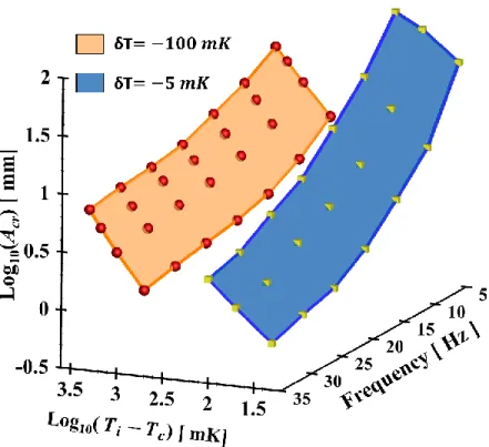
One of the primary motivations to analyse SCFs under thermo-vibrational instabilities has been to gain insights into the type of instabilities one may expect at different frequencies and amplitudes of vibration. While these instabilities may be used in certain processes to our advantage, for example mixing, in others, it may be desired to isolate the system to these instabilities. The authors in Ref. [23] presented a plot limited by the use of low q (10%, due to the use of a linear state equation). As the current model makes it possible to analyse the system with a higher quench percentage, a similar plot is presented in Fig. 17 (a-b). It is presented as a function of different q and for two different proximities to the critical point, and .

The plot illustrates that for amplitudes below the lower plane, the system will be stable with respect to both the described instabilities. Similarly, for amplitude bounded by the two planes, Rayleigh-vibrational instabilities will be first observed, while above the upper plane, both instabilities will occur simultaneously. Thus, it can be observed that higher amplitudes are required for the onset of parametric instabilities in both cases. The corresponding illustrations have been presented in Fig. 19 showing various instabilities depending on the operating parameters ( ) as marked in the figure itself.

33 Figure 17. Stability plot describing critical amplitude for onset of Rayleigh-vibrational and parametric instabilities as a function of quench percentage and frequency.

While it can be intuitively ascertained that it is easy to destabilize the fluid layers in parallel due to shear, it can be explained by analytical reasoning based on the mechanism causing both these instabilities. The Bernoulli-like pressure in Rayleigh-vibrational instabilities is observed to grow with the square of the velocity difference while in parametric, owing to the momentum transfer, it will follow a linear relation with velocity. Furthermore, since the momentum transfer occurs between two highly compressible fluids, some of the momentum is also expended in compressing the fluid whereas no such loss can be ascertained in case of Rayleigh-vibrational instabilities.

34 Figure 18. Stability plot illustrating different instabilities based on their operating conditions for

.

IV. Conclusion

The current work presents a 2D numerical investigation of thermo-vibrational instabilities in supercritical fluids under weightlessness, primarily Rayleigh-vibrational and parametric instabilities. These are observed when direction of vibration is normal and parallel to the temperature gradient, respectively. The primary feature of the current work pertains to investigation of these instabilities with higher quench percentages, as high as 50% and closer proximity to the critical point ( . This is facilitated by the use of a mathematical model that evaluates density directly from the mass conservation, incorporating the dependence of pressure on density and temperature directly into the momentum equation and thus is capable to take into account the non-linear variations of pressure with temperature and density. A comparison with experimental observations shows a close match demonstrating the strength of the model to investigate system with large property variations.

It is found that it is possible to define, for both the instabilities, a critical amplitude for their onset which decrease with an increase in the quench percentage and frequency of vibration. The analysis of dynamic behaviour of wavelength in Rayleigh-vibrational configuration shows an interesting observation wherein an increase in wavelength at higher acceleration is observed

35

irrespective of quench percentage. A new trend for Rayleigh-vibrational number covering a wider span in terms of proximity and quench temperatures is also observed. In case of parametric instabilities, it is found that the vibration critical amplitude depends on the cell size. While for low quench percentage, it is observed that the decrease in wavelength with acceleration nearly matches the trend as in the case of Faraday instabilities in immiscible fluids, a faster decreasing trend is observed at higher quench percentage which can be ascribed to dominance of non-linear effects at higher quench percentage. Finally, a stability plot highlighting critical regions in terms of thermo-vibrational parameters (quench percentage, frequency and critical amplitude) is presented wherein it is found that critical amplitude for onset of Rayleigh-vibrational instabilities is lower as compared to that of parametric instabilities.

References

[1] H. E. Stanley, Introduction to Phase Transitions and Critical Point Phenomena (Oxford University Press, Oxford, 1971).

[2] G. Lorentzen and J. Pettersen, International Journal of Refrigeration 16, 4 (1993).

[3] T. Rothenfluh, M. J. Schuler, and P. R. von Rohr, The Journal of Supercritical Fluids 57, 175 (2011).

[4] T. Neill, D. Judd, E. Veith, and D. Rousar, Acta Astronautica 65, 696 (2009).

[5] M. Pizzarelli, F. Nasuti, and M. Onofri, The Journal of Supercritical Fluids 62, 79 (2012).

[6] Ž. Knez, E. Markočič, M. Leitgeb, M. Primožič, M. Knez Hrnčič, and M. Škerget, Energy 77, 235 (2014).

[7] B. Zappoli, D. Beysens, and Y. Garrabos, Heat Transfers and Related Effects in Supercritical Fluids (Springer Netherlands, 2014), 1 edn., Vol. 108, Fluid Mechanics and Its Applications. [8] K. Nitsche and J. Straub, in Proceedings of the 6th European Symposium on Material Sciences

under Microgravity Conditions (ESA SP 256, 1987), pp. 109.

[9] A. Onuki and R. A. Ferrell, Physica A: Statistical Mechanics and its Applications 164, 245 (1990).

[10] H. Boukari, J. N. Shaumeyer, M. E. Briggs, and R. W. Gammon, Physical Review A 41, 2260 (1990).

[11] B. Zappoli, D. Bailly, Y. Garrabos, B. Le Neindre, P. Guenoun, and D. Beysens, Physical Review A 41, 2264 (1990).

[12] Y. Garrabos, D. Beysens, C. Lecoutre, A. Dejoan, V. Polezhaev, and V. Emelianov, Physical Review E 75, 056317 (2007).

[13] A. Jounet, A. Mojtabi, J. Ouazzani, and B. Zappoli, Physics of Fluids 12, 197 (1999).

[14] R. Wunenburger, P. Evesque, C. Chabot, Y. Garrabos, S. Fauve, and D. Beysens, Physical Review E 59, 5440 (1999).

[15] Daniel A Beysens, Régis Wunenburger, C. C. and, and Y. Garrabos., Microgravity - Science and Technology 11, 113 (1998).

[16] R. Wunenburger, D. Chatain, Y. Garrabos, and D. Beysens, Physical Review E 62, 469 (2000). [17] A. Mailfert, D. Beysens, D. Chatain, and C. Lorin, Eur. Phys. J. Appl. Phys. 71 (2015).

[18] T. Lyubimova, A. Ivantsov, Y. Garrabos, C. Lecoutre, G. Gandikota, and D. Beysens, Physical Review E 95, 013105 (2017).

36 [19] G. Gandikota, D. Chatain, S. Amiroudine, T. Lyubimova, and D. Beysens, Physical Review E 89,

013022 (2014).

[20] G. Gandikota, D. Chatain, T. Lyubimova, and D. Beysens, Physical Review E 89, 063003 (2014). [21] D. Chatain, SBT-INAC, CEA-Grenoble, private communication (2017).

[22] S. Amiroudine and D. Beysens, Physical Review E 78, 036325 (2008).

[23] G. Gandikota, S. Amiroudine, D. Chatain, T. Lyubimova, and D. Beysens, Physics of Fluids 25, 064103 (2013).

[24] S. Amiroudine, J. P. Caltagirone, and A. Erriguible, International Journal of Multiphase Flow 59, 15 (2014).

[25] D. Sharma, A. Erriguible, and S. Amiroudine, Physical Review E 96, 063102 (2017).

[26] E. Ahusborde and S. Glockner, International Journal for Numerical Methods in Fluids 62, 784 (2010).

[27] A. Poux, S. Glockner, and M. Azaïez, J. Comput. Phys. 230, 4011 (2011). [28] D. Sharma, A. Erriguible, and S. Amiroudine, Phys. Rev. E 96, 063102.

[29] D. Sharma, A. Erriguible, and S. Amiroudine, Theoretical and Computational Fluid Dynamics 31, 281 (2017).

[30] D. Sharma, A. Erriguible, and S. Amiroudine, Physics of Fluids 29, 126103 (2017).

[31] P. R. Amestoy, I. S. Duff, and J. Y. L'Excellent, Computer Methods in Applied Mechanics and Engineering 184, 501 (2000).

[32] G. Z. Gershuni and A. V. Lyubimov, Thermal Vibrational Convection (Wiley, New York, 1998). [33] K. Kumar and L. S. Tuckerman, Journal of Fluid Mechanics 279, 49 (1994).

[34] V. Shevtsova, Y. A. Gaponenko, V. Yasnou, A. Mialdun, and A. Nepomnyashchy, Journal of Fluid Mechanics 795, 409 (2016).

Appendix

The Navier–Stokes equations presented in Sec. II are discretized using finite volume method on a staggered Cartesian grid. The general time-discretization algorithm can be described as follows. The initial conditions for the flow variables ( ) are given in the problem formulation.

Step 1: The momentum equation (Eq. (2)) is discretized with forward first order Euler in time.

37

₍₆₎

Step 2: In order to evaluate the pressure field, Eq. (4) is integrated over the time step of

simulation, , following which it can be written as,

(7)

It is worth mentioning here that in the above Eq. (7), we have simplified However, this simplification is not ascribed to the assumption that the divergence of the velocity field is independent of time. It is more of a numerical simplification, where for the time step , the integral can be simplified using several possible choices such as, , or using Simpsons rule etc. Since no difference in the results is obtained with either choice, we have used the aforesaid approximation. Thus, from Eq. (7), the expression for pressure at time step is directly incorporated into the momentum equation, Eq. (6) following which it can be written as,

(8)

This highlights a very important step of the developed model wherein the dependence of pressure on density (through ) is directly incorporated in the momentum equation with the implicit contribution of the velocity field.

38

Step 3: The pressure is updated using Eq. (7) utilising the velocity field obtained by solving Eq. (8).

Step 4: The updated velocity field is then used to implicitly evaluate the temperature field

at by discretizing the energy equation Eq. (3) (in the absence of source term and viscous dissipation) as,

(9)

Step 5: The updated velocity field at is further used to evaluate the density at time

step using the following relation (integrating the last part of Eq. (1)),

₍₁₀₎

Step 6: The fields of the variables are then advected from their respective total derivatives (see

Eq. (5)) through the TVD scheme. The updated values of temperature _{are then used to}

evaluate thermo-physical properties as described in Table I to be used in next iteration. The above process is repeated in time by setting the values at time to the values at time