Analysis of PV Drains for Mitigation of Seismically
Induced Ground Deformations in Sand Slopes
The MIT Faculty has made this article openly available. Please share how this access benefits you. Your story matters.Citation Vytiniotis, Antonios, and Andrew J. Whittle. “Analysis of PV Drains for Mitigation of Seismically Induced Ground Deformations in Sand Slopes.” Journal of Geotechnical and Geoenvironmental Engineering 143, 9 (September 2017): 04017049
As Published http://dx.doi.org/10.1061/(ASCE)GT.1943-5606.0001722
Publisher American Society of Civil Engineers (ASCE)
Version Author's final manuscript
Citable link http://hdl.handle.net/1721.1/117512
Terms of Use Creative Commons Attribution-Noncommercial-Share Alike
1
ANALYSIS OF PV DRAINS FOR MITIGATION OF SEISMICALLY-INDUCED 1
GROUND DEFORMATIONS IN SAND SLOPES 2
by 3
Antonios Vytiniotis1, M. ASCE, P.E. & Andrew J. Whittle2, M. ASCE, P.E.
4 5
ABSTRACT: Prefabricated Vertical (PV) drain arrays have been proposed as a minimally-6
intrusive technique for mitigating seismically-induced ground deformations in sandy liquefiable
7
slopes. This paper describes the representation of individual PV drains as line elements within the
8
OpenSees finite element program. The elements can represent laminar or fully-turbulent discharge
9
regimes, based on classic Darcy-Weisbach pipe flow, as well as fluid storage above the water table.
10
Two-dimensional, plane strain simulations of coupled flow and deformation are performed using
11
the proposed PV drain elements, with equivalent permeability properties for the surrounding soil
12
mass, and the Dafalias-Manzari (DM2004) model to describe non-linear effective stress-strain
13
behavior of the sand. The numerical predictions are evaluated through comparisons with pore
14
pressures and deformations measured in a centrifuge model test. The results highlight the role of
15
the PV drains and their discharge characteristics in controlling deformation mechanisms.
16
Keywords: Finite element analysis, earthquake engineering, centrifuge scale modeling, hazard
17
mitigation, PV drains
18
1 Exponent Failure Analysis Inc., 9 Strathmore Rd, Natick, MA, 01760, e-mail: [email protected] 2 Professor, Massachusetts Institute of Technology, 77 Massachusetts Avenue, Cambridge, MA, 02139
2
INTRODUCTION 1
There are a variety of soil improvement methods that can be used to reduce liquefaction
2
susceptibility of loose sands. Most of the standard methods rely on some form of mechanical
3
improvement of the soil mass through either in situ densification methods such as dynamic
4
compaction (Mitchell et al., 1995), vibroflotation, vibro-replacement and cementation methods
5
such as jet grouting, deep soil mixing, or compaction grouting (Adalier et al., 1998; Priebe, 1998;
6
Miller and Roycroft, 2004; Boulanger and Hayden, 1995), or stone/gravel columns (e.g., Seed and
7
Booker, 1977), which enhance drainage and also strengthen the soil mass. Some of these
8
techniques produce significant disturbance within the soil mass and hence, have limited
9
applicability in retrofit projects. In contrast, a number of ‘minimally intrusive’ liquefaction
10
mitigation techniques have also been proposed including PV drains, (Rathje et al., 2004; Rollins
11
et al., 2003) and permeation grouting using colloidal silica that forms a gel within the pore space
12
(Gallagher and Mitchell, 2002, Diaz-Rodriguez et al., 2008). While the effectiveness of these
13
techniques have been demonstrated through physical and full-scale model tests (e.g., Rollins et al.,
14
2003; Gallagher et al., 2007; Howell et al., 2012; Marinucci et al., 2008; Kamai et al., 2008), there
15
remains a lack of validated design methods for these methods of ground improvement.
16
This paper focuses on the effectiveness of PV drain systems for mitigating liquefaction and
17
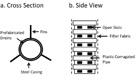
cyclic mobility in sloping sand fills. The PV drains proposed for this application comprise high
18
flow capacity, perforated plastic pipes (with inside diameter, D= 75mm – 200mm) that are encased
19
in geosynthetic filter fabric (Figure 1). The drains are typically installed in a grid pattern using a
20
mandrel that is vibrated into the ground and then withdrawn. The drain spacing, de, is currently
21
designed to limit the development of excess pore pressures (ru,max = |Δp/σ'v0|max where p is the pore
22
pressure, and σ'v0 the initial in situ vertical effective stress) within the soil. This is achieved by
3 balancing the undrained generation and dissipation of excess pore pressures during a design
1
earthquake, characterized in this study by the bracketed duration of the event, td, the equivalent
2
number of uniform shear stress cycles of loading, Neq, and the number of uniform cycles of
3
undrained shearing of a representative magnitude necessary to cause initial liquefaction, Nl.
4
Seed and Booker (1977) proposed analyses for the case of gravel drains assuming radial
5
flow within a homogeneous soil mass and infinite vertical drain transmissivity (‘perfect sink’
6
representation). They developed design charts linking the maximum excess pore pressure ratio,
7
ru,max, to the spacing ratio, rs = D/de, the time factor associated with the normalized duration, Tad =
8
4Cvtd/((D)2), and seismic loading conditions (rn=Neq/Nl) of the design earthquake as shown in
9
Figure 2.
10
Onoue (1988) subsequently modified the design charts to include well resistance as an
11
important factor affecting the performance of gravel drains, a feature confirmed by Boulanger et
12
al. (1998) who also found significant changes in drain permeability due to transport of fine
13
particles. Pestana et al. (1998) developed a more general non-linear numerical analysis program
14
(FEQDRAINTM) following the same principles. This program specifically accounts for the head
15
loss of the fluid flowing across the walls and along a PV drain, together with a range of boundary
16
conditions that control the storage of water within the drain (drain storage capacity) and discharge
17
at the ground surface as illustrated in Figure 3.
18
None of the existing design methods consider how the PV drains affect deformations within
19
the soil mass. This is clearly a major limitation in evaluating their effectiveness as a mitigation
20
solution, especially in sloping ground. This paper investigates the performance of PV drain
21
systems through 2-D finite element analyses of coupled flow and deformation using the OpenSees
22
program (Mazzoni et al., 2005). The analyses simulate PV drains using a new class of 1-D line
4 elements that can represent laminar or tubulent pipe flow regimes, while radial seepage from the
1
surrounding soil is approximated using equivalent hydraulic conductivity properties (after Hird et
2
al., 1992). Non-linear effective stress-strain behavior of the sand is represented using the DM2004
3
model proposed by Dafalias and Manzari (2004). This paper evaluates predictive capabilities of
4
the analyses using data from a centrifuge model test (SSK01; Kamai et al., 2008). The results
5
show how the assumed PV flow regime affects the predicted drainage conditions within the soil
6
mass, while comparisons with the measured data are used to understand how drainage limits lateral
7 spreading. 8 9 PV-DRAIN ELEMENTS 10
Full-bore flow inside pipes (such as PV-drains) is commonly modeled through the
Darcy-11
Weisbach equation that relates the frictional pressure loss, Δp, to the average fluid velocity, v. For
12 a circular pipe: 13 Δ𝑝 = 𝜆 ⋅𝐿 𝐷⋅ 𝜌𝑣2 2 (1)
where L and D are the length and inner diameter of the pipe respectively, ρ the mass density of
14
water, and λ is a dimensionless friction factor controlled by the wall roughness and Reynolds
15
number, Re (where Re = vD/with μ being the dynamic viscosity of the draining fluid after
16
Moody (1944).
17
For laminar flow (Re < 2300), the friction coefficient is inversely proportional to Re (=
18
64/ Re) and using equation (1) the flow rate can be written in a rate form:
5 𝑄 = 𝐶𝑙Δ𝑝 𝐿 (2a) 𝑄̇ = 𝐴𝑓⋅ 𝐷 2 32 ⋅ 𝜇 ⋅ 𝐿Δ𝑝̇ = 𝐶𝑙 𝐿 Δ𝑝̇ (2b) 1
where Af is the wetted area (i.e., D2/4 for full-bore flow) of the drain and the laminar drain
2
coefficient, Cl = AfD2/32.
3
Similarly, in the fully turbulent regime, the friction factor is constant and is controlled
4
by the wall roughness. The flow can be expressed as:
5 𝑄 = 𝐶𝑡√Δ𝑝 𝐿 (3a) Q̇ = √2 ⋅ 𝐷 ⋅ 𝐴𝑓 2 𝜆 ⋅ 𝐿 ⋅ 𝜌 ⋅ 1 2√Δ𝑝⋅ Δ𝑝̇ = 𝐶𝑡 1 2√Δ𝑝L Δ𝑝̇ 𝐿 (3b)
where the fully turbulent drain coefficient, 𝐶𝑡 = √2 ⋅ 𝐷 ⋅ 𝐴𝑓2/(𝜆 ⋅ 𝜌).
6
The current analyses represent the PV drains as one-dimensional extended elements within
7
the OpenSees finite element program (Mazzoni et al., 2005). This approach implicitly decouples
8
the pipe flow from mechanical deformations of the drains (the current study does not consider
9
possible buckling of drains). Fluid pressures inside the pipe are assumed to match the external pore
10
pressures in the adjacent soil (i.e., there is no allowance for head loss through the pipe wall), and
11
the bending stiffness of the thin-walled drains is negligible. The resulting two-noded PV drain
12
elements have three degrees of freedom per node as shown in Figure 4, with generalized force and
13
displacement vectors given by:
6 𝑞̂ ̇ =[𝑞1̇ 𝑞2̇ 𝑄1̇ 𝑞3̇ 𝑞4̇ 𝑄2̇ ]𝑇 (4a)
𝑢̂̇ = [𝑢1̇ 𝑢2̇ 𝑝1 ̇𝑢3̇ 𝑢4̇ 𝑝2̇ ]𝑇 (4b)
where 𝑢𝑖̇ and 𝑞𝑖̇ are the rates of nodal displacement and force components respectively; 𝑝𝑖̇ and 𝑄̇ 𝑖
1
are the rates of nodal pore pressures and axial flow respectively.
2
The generalized equilibrium of the finite element can be written:
3 [ 𝑞1̇ 𝑞2̇ 𝑄1̇ 𝑞3̇ 𝑞4̇ 𝑄2̇ ] = [ 𝑘11 𝑘12 0 −𝑘11 −𝑘12 0 𝑘12 𝑘22 0 −𝑘12 −𝑘22 0 0 0 𝑘33 0 0 −𝑘33 −𝑘11 −𝑘12 0 𝑘11 𝑘12 0 −𝑘12 −𝑘22 0 𝑘12 𝑘22 0 0 0 −𝑘33 0 0 𝑘33 ] ⋅ [ 𝑢1̇ 𝑢2̇ 𝑝1̇ 𝑢3̇ 𝑢4̇ 𝑝2̇ ] (5) where 𝑘11= cos2𝜃 ⋅𝐴𝐸 𝐿 ; 𝑘12= cos 𝜃 ⋅ sin 𝜃 ⋅ 𝐴𝐸 𝐿 ; 𝑘22= sin 2𝜃 ⋅𝐴𝐸
𝐿 ; and AE is the axial stiffness
4
of the thin-walled PV drain, and θ its orientation in the global coordinate system.
5
The formulation is completed through the definition of k33 that defines the
incrementally-6
linearized relationship between pore pressure and flow rate. In the laminar regime this is obtained
7
directly from the drain coefficient:
8 𝑘33= − 𝐴𝑓⋅ 𝐷2 32 ⋅ 𝜇 ⋅ 𝐿 = −𝐶𝑙⋅ 1 𝐿 (6)
In the fully turbulent regime the pressure-flow rate relation is non-linear. The numerical
9
implementation considers an increment in the nodal water pressures at time i, and the resulting
10
flow rate in this time step, Qi:
11
δ𝛥𝑝i = δ𝑝𝑖2− δ𝑝𝑖1 (7a) δQi = 𝑄(𝛥𝑝𝑖 + 𝛿𝛥𝑝𝑖) − 𝑄(𝛥𝑝𝑖) (7b) From which the ‘consistent’ stiffness coefficient can be derived:
12
𝑘33𝑖 = δ𝑄
𝑖
7 This approach can generate numerical problems when the pore pressure difference or
1
incremental pressure difference are very small (i.e., Δpi≈ 0; δΔpi≈ 0, thus the denominator is very
2
close to zero). These cases are avoided by specifying a threshold pressure difference, dc, with the
3
following approximations as illustrated in Figure 4 (shown for Δpi > 0, without any loss of
4 generality): 5 δΔ𝑝i < dc ∩ Δ𝑝i > dc: 𝑘33𝑖 = √2 ⋅ 𝐷 ⋅ 𝐴𝑓 2 𝜆 ⋅ 𝐿 ⋅ 𝜌 ⋅ 1 2√Δ𝑝𝑖 δΔ𝑝i < dc ∩ Δ𝑝i < dc: 𝑘33𝑖 = 𝐶𝑡 √𝑑𝑐⋅ 𝐿 (8b) (8c)
We implemented the two element classes (i.e., laminar and fully turbulent regimes) within
6
the OpenSees code. In practice, the groundwater table often lies well below the ground surface
7
and PV drains are installed through overlying, partially saturated soil units. A variety of boundary
8
conditions can be expected depending on the permeability of these surficial layers. This paper also
9
considers the case where the surficial soils have low permeability and water fills the PV drain
10
before discharge occurs at the ground surface. The storage capacity of each PV drain corresponds
11
to the volume of fluid stored above the water table prior to discharge. As the proposed PV drain
12
elements compute flow at every time-step, the total influx of water can be used to update the
13
location of the water table inside the drain (H, Figure 3) and hence, the pore pressure at Point A.
14
Representation of Drains in 2-D analyses 15
Hird et al. (1992) have investigated the use of two-dimensional, plane strain finite element
16
(FE) analyses for simulating quasi-static consolidation with arrays of PV drains. They show that a
17
plane strain unit cell can achieve the same average degree of consolidation as an axisymmetric unit
18
cell through the selection of an equivalent drain spacing, or through equivalent soil permeability
8 and equivalent drain transmissivity. When the drain spacing is the same in the axi-symmetric and
1
plane strain configurations then the three dimensional flow can be matched in the plane strain
2
model using an equivalent permeability of the soil, kpl, as follows:
3
𝑘pl = 2𝑘𝑎𝑥
3[ln(1/𝑟𝑠) − 3/4] (9)
where kax is the permeability for the physical situation and rs is the drain spacing ratio.
4
An equivalent drain transmissivity also needs to be introduced to match the same average
5
degree of consolidation. By solving analytically the plane strain and axisymmetric horizontal flow
6
towards a drain in a unit cell, the equivalent plane strain laminar flow coefficient can be
7 approximated as: 8 𝐶𝑙𝑝𝑙 = 2 𝜋𝑅𝐶𝑙 𝑎𝑥 (10)
The Appendix shows that the turbulent flow coefficient can be approximated linearly to
9
the laminar flow coefficient for a range of pressures gradients, thus the equivalent plane strain
10
fully turbulent flow coefficient can be approximated as (for a plane strain grid of width w):
11
𝐶𝑡𝑝𝑙 = 2 𝜋𝑅𝐶𝑡
𝑎𝑥√𝑤 (11)
12
Vytiniotis (2009) has confirmed that this approach achieves very close matching of the
13
average degree of consolidation, there are differneces in the spatial distribution of excess pore
14
pressures between the equivalent plane strain and radial drainage models. The current analyses
15
tend to overestimatethe excess pore pressures mid-way between drains. However, this discrepancy
16
is readily justified by the large computational advantage associated with the 2D model.
9 The Appendix shows that in order to appropriately scale efflux rates through a PV drain
1
between prototype and model scales it is important to consider the specific flow regimes (i.e.,
2
laminar vs. turbulent). If appropriate efflux scaling is used, the Reynolds number (Re) differs
3
between the scale-model and prototype (assuming the same fluid is used in both cases). Thus, it is
4
possible that turbulent flow in a prototype PV drain can correspond to laminar flow at model-scale.
5
Given this discrepancy, the Appendix proposes a methodology to design model-scale PV drains
6
that match the flow in prototype scale drains more accurately and to evaluate, a priori, the effect
7
of turbulence on drain outflow rates.
8 9
EVALUATION OF NUMERICAL FRAMEWORK USING CENTRIFUGE MODEL 10
The numerical procedures dealing with the simulation of the PV-drains have been validated
11
through finite element modeling of a reference centrifuge model test, SSK01 (Kamai et al., 2008)
12
conducted in the 9-meter radius centrifuge at University of California (UC) Davis operating at a
13
gravitational acceleration of 15 g (N=15). The test compares the response of two similar facing
14
slopes with a central channel (Figure 5). Beneath the left side slope, is a layer of loose sand
15
containing an array of perforated nylon PV-drains, while the right side slope is underlain by
16
untreated, loose sand. The model PV drains were placed prior to pluviation of the surrounding
17
sand and hence, there are no local densification effects associated with drain installation. The two
18
sides both comprise three distinct soil layers: 1) a base layer of dense fine Nevada Sand, with
19
relative density, Dr=84%; 2) a “liquefiable” layer of loose Nevada Sand, Dr=40%; and 3) a cap
20
layer of compacted (low permeability) Yolo Loam.
10 Nevada sand is a fine sand (D50=1 mm, γd,max=17.33 kN/m3, γd,min=13.87 kN/m3) and was
1
placed by dry pluviation. The Yolo Loam is a clayey silt (with plasticity index, Ip = 13%) and was
2
placed in multiple lifts compacted by gentle tamping. It impedes vertical dissipation of pore water
3
from the liquefiable layer.
4
The model was subjected to a sequence of five harmonic shaking events with period, T=0.5s,
5
and maximum accelerations amax=0.01, 0.03, 0.07, 0.11, 0.3g. All events were applied transverse
6
to the central channel in the longitudinal direction. Figure 5a illustrates part of the model
7
instrumentation that included i) arrays of accelerometers and pore-pressure transducers within the
8
loose sand; and ii) displacement transducers to measure vertical and horizontal displacements at
9
the surface of the Yolo loam. The current analysis considers only the third loading sequence
10
(named SSK01_10) with maximum applied horizontal acceleration, amax=0.07g. This is the first
11
event involving significant generation of excess pore pressures and ground deformations and
12
hence, the most credible for model validation.
13 14
Finite Element Model 15
The finite element analysis is performed at prototype scale. Figure 5b illustrates the main
16
features of the OpenSees finite element model used to simulate the centrifuge model test:
17
1. Coupled flow and deformation in the high permeability sand layers are represented by 4-noded
18
QuadUP elements with bilinear interpolation of displacements and pore pressures. Although
19
these elements have limitations when modeling incompressible behavior (i.e., they do not
20
satisfy Babuska-Brezzi conditions for undrained shearing of saturated soil; cf., Oden and
21
Carey, 1984), the Authors have found no problems in the current analyses where partial
11 drainage prevails throughout the sand layer. The element size was selected to be approximately
1
0.2m in order to prevent aliasing of seismic waves based on the known frequency of the applied
2
excitation and computed stiffness properties of the soils. The high spatial resolution also
3
enables good interpolation of deformations and pore pressures between the lines of PV drains.
4
The effective stress-strain-strength properties of the Nevada sand layers are modeled using the
5
DM2004 model (with parameters described in the next section).
6
2. Time stepping is accomplished using the Krylov subspace acceleration Newton algorithm
7
(Scott & Fenves, 2010). The time step-size was varied dynamically in order to achieve
8
efficient convergence to the specified energy error norm. Numerical accuracy was established
9
by comparing the computed results over a range of tolerances.
10
3. The capping layer of Yolo loam is represented by 4-noded Quad elements (bi-linear
11
displacement interpolation using total stresses), and its undrained shear properties are
12
represented by an elastic, perfectly-plastic model (Mazzoni et al., 2005).
13
4. Displacements of contact nodes between QuadUP and Quad domains are tied together (i.e.,
14
there is no slippage between the sand and the loam layers).
15
5. The centrifuge model is built within a laminar box (flexible shear beam container). Periodic
16
boundary conditions are applied at the sides of the model (including the mass of the steel
17
plates). The sand layers are continuous across the model and hence, remain in contact with the
18
box walls throughout shaking. In contrast, the Yolo loam forms a partial cap and is absent in
19
the central channel.
20
6. The PV drain array is represented in the 2D numerical model by a series of 7 uniformly-spaced,
21
lines of laminar or turbulent flow drain elements with properties listed in Table 1. The water
12 table is located at the top of the sand layer in the centrifuge model, while the PV drains
1
discharge at the ground surface (i.e., above the Yolo loam). Hence, there is a significant storage
2
effect (i.e., water will move upwards in the PV-drains before discharging at the ground surface
3
and effectively reducing excess pore pressures in the sand layers) that is also represented by
4
the drain elements. The finite element approximation of planar flow is represented using an
5
equivalent hydraulic conductivity. There is free flow occurring towards the central channel and
6
closed flow boundaries along the sides and the base of the model. The sand is assumed to have
7
in prototype scale a hydraulic conductivity of kp = 3x10⁻⁴ m/s in the untreated region, and kp =
8
1x10⁻⁴ m/s in the improved region to match the properties for radial flow into the drain. The
9
input parameters needed for the PV drains are the transmissivity for laminar flow, the
10
transmissivity for turbulent flow, the axial stiffness, and the storage capacity. The nylon drains
11
have an inner diameter, Dp = 105 mm, and wall thickness, wp = 30 mm (prototype scale). Table
12
1 summarizes the input parameters for the PV-drains at prototype scale, corresponding to a
13
centrifuge model scaling factor, N=15.
14
7. Seismic loading is represented by applying a uniform horizontal excitation (acceleration)
15
across the base of the model.
16
Soil Parameters 17
Although there are some uncertainties in the as-built density of the centrifuge model, the
18
current analyses assume that the dense and loose Nevada sand are prepared uniformly with relative
19
densities, Dr = 80% and 40% respectively. The DM2004 critical state elasto-plastic constitutive
20
soil model is used to simulate the effective stress-strain properties of the sand during cyclic loading
21
events. This model predicts reasonably well both the monotonic and the cyclic behavior of sand
22
measured in laboratory element tests and is also able to capture the effects of void ratio and
13 confining stress with a single set of model input parameters. It simulates shear-induced volumetric
1
plasticity during loading and subsequent unloading paths. Input parameters for the DM2004
2
effective stress model have been calibrated for fine Nevada sand by Vytiniotis (2012) (Table 2)
3
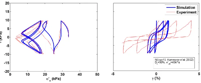
and are used in the current numerical simulations. Figure 6 shows a typical comparison between
4
computed and measured behavior of medium-loose Nevada sand (Dr = 50%; Kammerer et al.,
5
2000) for two-way cyclic undrained direct simple shear test, at an initial confining stress, σ'vc=35
6
kPa. These results show reasonable agreement between the computed and measured effective
7
stress paths (i.e., accumulation of shear-induced pore pressures; Fig. 6a). The model also
8
accumulates shear strain with load cycles (Fig. 6b) but reaches a shakedown condition after 4 load
9
cycles (while the measured data shows further strain accumulation with little change in excess pore
10
pressure) number of cycles. For cases with an initial static shear stress, the DM2004 model can
11
also predict continuous accumulation of plastic strains, but the accuracy is varies with the obliquity
12
of the initial stress state (Vytiniotis, 2012).
13
The DM2004 model was implemented in the OpenSees software framework by the authors using
14
an explicit integration scheme with automatic sub-incrementation. To further improve the
15
integration of the model, a correction algorithm that returns the model state to the critical state or
16
the bounding surface line (whichever one is controlling based on the state of the sample) was
17
implemented as suggested by Potts and Gens (1985). Finally, a return-to-apex correction was
18
implemented. Vytiniotis (2012) presents full details of the model implementation.
19
Undrained shear properties of the Yolo loam are represented by an elasto-plastic model, with
20
shear stiffness dependent on the effective confining stress, and shear strength described by a von
14 Mises yield criterion with associated flow (using the PI-MYS nested yield model available in
1
OpenSees, Mazzoni eta l., 2005). Table 3 lists the input parameters for this model.
2
3
Interpretation and Evaluation of Computed Results 4
Laminar vs. Turbulent Drains
5
Figure 7 compares the computed pore pressures for the SSK01_10 event (i.e., amax=0.07 g)
6
using laminar and turbulent drain elements at three elevations within the loose sand. As expected,
7
there is greater accumulation of excess pore pressures in the lower sand on the untreated side of
8
the model (F vs C). Differences in modeling the flow regimes have little effect on the untreated
9
side of the model (points D, E, F). However, within the treated zone, pore pressures accumulate
10
more rapidly for the analyses with fully turbulent PV drain elements showing that laminar flow
11
assumption can lead to non-conservative results (i.e., greater computed pore pressure dissipation).
12
At point C the analyses predict significantly higher excess pore pressures for turbulent drains as
13
turbulence diminishes the discharge capacity of the PV-drains.
14
Drain Outflow
15
Figure 8 shows typical outflow results computed for one row of drains (#2, see Figure 5)
16
during the cyclic loading event (t ≤ td = 10 secs) and subsequent dissipation (3 secs). As discussed
17
in the Appendix, when a scale model is designed so that the same excess pore pressures generation
18
and dissipation occurs at model and prototype scales, the Reynolds numbers do not scale
19
accordingly. Figure 8a shows that the calculated efflux of a single row of drains is above the
20
laminar limit for a prototype scale model but remains just marginally above laminar if model-scale
21
flow is considered. Thus in this simulation a fully-turbulent assumption would reduce the effective
15 permeability of the drains. For this reason, subsequent comparisons of simulations and
1
experimental data are based on the laminar drain analysis.
2
This result also highlights the need to consider carefully the design of model-scale PV
3
drains that appropriately simulate prototype-scale flow (using the procedure described in the
4
Appendix). Figure 8b shows that, despite the cyclic nature of the loading the discharged volume
5
increases steadily during the shaking event due to the continuous accumulation of excess pore
6
pressures within the loose sand.
7
Soil Behavior
8
Figure 9 examines the effective stress paths (σ'v,τw) and stress-strain (τw,γ) behavior at three
9
points in the middle of the loose sand layer. Point A is midway between two PV-drains, B is
10
adjacent to a PV drain, and C is located on the untreated side of the model (at the same elevations).
11
Points A and C show similar behavior; the vertical effective stress decreases in each load cycle,
12
and is constrained by the frictional strength of the sand (φ = 31°). Shear strains accumulate in each
13
load cycle with diminishing levels of shear resistance. Point C reaches a state of “liquefaction”
14
where σ'v0 and shows a notable amplification in cyclic shear strain with load cycles. There is a
15
much smaller build-up of excess pore pressure, Δu=-Δσ'ν , at point B indicating that flow towards
16
the PV-drains acts to stabilize the response of the loose sand and produces smaller accumulation
17
of shear strains.
18
Comparisons with Measurements: Predicted Excess Pore Pressures
19
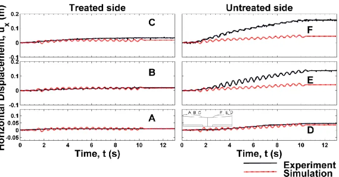
Figure 10 compares the predicted and measured pore pressures at six points within the
20
loose sand. It is readily apparent from the measured data that PV drains are effective in reducing
16 excess pore pressures generated within the sand (compare time series for A vs. D at the top, B vs.
1
E in the middle or C vs. F towards the base of the sand).
2
The numerical analyses provide good predictions of the measured excess pore pressures in
3
the middle part of the untreated sand, E, but they underestimate the pore pressures occurring at the
4
top of the untreated sand, point D. This result occurs, in large part, because the ground water level
5
does not remain constant during the experiment due to sliding of the Yolo loam cap towards the
6
central channel (Kamai et al., 2008). It is also possible that the pore pressure transducer sank as
7
the untreated sand underwent liquefaction during the test.
8
The numerical analyses also predict slower dissipation of excess pore pressures after
9
cessation of shaking at point E, a feature that is related to the selected consolidation coefficient
10
(i.e., post shaking stiffness of the sand and its hydraulic conductivity) in the sand. There is
11
uncertainty in the actual value of the hydraulic conductivity of the placed sand layers and in its
12
variation during and after base shaking. At the bottom of the model (point F) the analysis
13
overpredicts excess pore pressures because closed flow boundaries misrepresent partial drainage
14
occurring at the sand/laminar box interface.
15
On the treated side of the model, direct comparison of the computed and measured pore
16
pressures (points A, B and C) should be interpreted with caution, since the plane strain analyses
17
match the average degree of consolidation in the sand surrounding the drains, not the spatial
18
variation of excess pore pressures (Vytiniotis, 2012). The equivalent plane strain analyses
19
generally predict higher excess pore pressures than those expected for a model with 3D flow at the
20
midpoint between the PV- drains as shown via a comparison between axisymmetric and plane
21
strain equivalent analyses in Vytiniotis (2009). This trend appears to be consistent with results at
17 points B and C. However, the numerical model predicts smaller excess pore pressures than the
1
measured data at point A.
2
Displacements
3
Special care is needed when trying to interpret displacement measurements from centrifuge
4
model tests because of non-uniformities in the gravitational field that affect the measured
5
deformation mechanisms (Vytiniotis and Whittle, 2009). Figure 11 summarizes the computed and
6
measured horizontal deformations for a series of 6 points along the surface of the Yolo loam cap.
7
On the untreated side, the numerical analysis underestimates the lateral movements at points E and
8
F (due to tension cracks that were observed in the Yolo loam), but is in very reasonable agreement
9
with the experimental results at point D. On the treated side, the analysis results are in good
10
agreement with the smaller movements measured above the PV drains.
11
Figure 12 compares the simulated lateral deformations along two vertical sections (on the
12
treated and the untreated sides) at various times during shaking. For the untreated side, the results
13
show that lateral spreading within the loose Nevada sand is partially constrained by the overlying
14
Yolo loam cap. There is much smaller lateral spreading on the treated side of the model, confirming
15
the efficacy of the PV drains in mitigating effects of liquefaction. Since the drain elements have
16
no bending stiffness they have no effect on predicted lateral displacements.
17
Figure 13 compares the time-histories of the computed and measured vertical deformations at
18
6 points along the surface of the Yolo Loam. The finite element analyses correctly predict much
19
smaller surface settlements on the treated side (points A, B and C). The comparisons on the
20
untreated side vary from over-prediction at point F and E to relatively good agreement in point D.
18 Figure 14 shows that the numerical predictions of deformations are associated with a large
1
rotational mechanism on the untreated side of the model.
2
3
CONCLUSIONS 4
One-dimensional drain elements have been developed to represent laminar or fully turbulent
5
discharge through PV drains based on the Darcy-Weisbach pipe flow equation. The drain elements
6
are implemented in the OpenSees finite element framework. Scaling laws describing modeling of
7
PV drains in model-scale centrifuge experiments are presented. It is shown that the Reynolds
8
number in prototype-scale inside the PV drains can be different than the number in model-scale,
9
thus it is possible that the model-scale flow remains laminar whereas prototype flow is turbulent.
10
The Appendix gives guidelines for experimentalists to select an appropriate model-scale drain
11
dimensions that fits best the discharge of prototype drains.
12
The PV drain elements have been evaluated through comparisons with the measurements from
13
a centrifuge model consisting of a loose sand slope improved with a PV drain system under a cyclic
14
base excitation (event SSK01_10; Kamai et al., 2008). The numerical analyses incorporate the
15
DM2004 (Dafalias and Manzari, 2004) model to represent the cyclic effective stress-strain
16
properties of the loose Nevada sand. Overall, the numerical model provides reasonable qualitative
17
agreement with observed pore pressures in the centrifuge model. However, the computed results
18
are affected by uncertainties in the density and hydraulic conductivity of the loose sand layers and
19
by partial flow at the base boundaries through the laminar box-sand interface. Simulation results
20
further verify that flow towards the PV drains acts to stabilize the response of the loose sand and
21
leads to smaller accumulation of shear strains in a slope improved with PV drains. Numerical
19 analysis indicates that, within the treated zone, pore pressures accumulate more rapidly for the
1
analyses with fully turbulent PV drain elements showing that laminar flow assumption can lead to
2 unconservative results. 3 4 ACKNOWLEDGEMENTS 5
The authors are grateful for support from NSF grant No. CMS-0530478, under the NEESR Grand
6
Challenge project, “Seismic Risk Management for Port Systems”. The computations were
7
performed on a cluster computer through the Center for Environmental Sensing and Modeling
8
(CENSAM), part of the SMART program in Singapore. The first author also received support
9
from the Alexander S. Onassis Public Benefit Foundation.
10 11
20
REFERENCES 1
Adalier, K., Elgamal, A. K., & Martin, G. R. (1998). “Foundation liquefaction countermeasures
2
for earth embankments.” Journal of Geotechnical and Geonenvironmental Engineering,
3
10.1061/(ASCE)1090-0241(1998)124:6(500).
4
Boulanger, R. W., Idriss, I. M., Stewart, D. P., Hashash, Y., & Schmidt, B. (1998). “Drainage
5
capacity of stone columns or gravel drains for mitigating liquefaction.” Geotechnical
6
Earthquake Engineering and Soil Dynamics III. 1, Eds. P. Dakoulas, M. Yegian, and R. D.
7
Holtz, 678-690.
8
Boulanger, R. W., & Hayden, R. (1995). “Aspects of compaction grouting of liquefiable soil.”
9
Journal of Geotechnical Engineering, 10.1061/(ASCE)0733-9410(1995)121:12(844).
10
Chiou, B., Darragh, R., Gregor, N., & Silva, W. (2008). “NGA project strong-motion database.”
11
Earthquake Spectra, 24(1), 23-44.
12
Dafalias, Y., & Manzari, M. (2004). “Simple plasticity sand model accounting for fabric change
13
effects”. Journal of Engineering Mechanics,
10.1061/(ASCE)0733-14
9399(2004)130:6(622).
15
Díaz-Rodríguez, J., Antonio-Izarraras, W., Bandini, P., & López-Molina, J. (2008). “Cyclic
16
strength of natural liquefiable sand stabilized with colloidal silica grout.” Canadian
17
Geotechnical Journal, 45, 1345-1355.
18
Gallagher, P., & Mitchell, J. (2002). “Influence of colloidal silica grout on liquefaction potential
19
and cyclic undrained behavior of loose sand.” Soil Dynamics and Earthquake Engineering,
20
22(9-12), 1017-1026.
21
Gallagher, P., Conlee, C., & Rollins, K. (2007). “Full-scale field testing of colloidal silica grouting
22
for mitigation of liquefaction risk.” Journal of Geotechnical and Geoenvironmental
23
Engineering, 10.1061/(ASCE)1090-0241(2007)133:2(186).
24
Hird, C. C., Pyrah, I. C., & Russell, D. (1992). “Finite element modelling of vertical drains beneath
25
embankments on soft ground.” Géotechnique, 42(3), 499-511.
26
Hosono, Y., & Yoshimine, M. (2004). “Cyclic behavior of soils and liquefaction phenomena.”
27
Processing of the International Conference on Cyclic Behavior of Soils and Liquefaction
28
Phenomena, 129-136. Bochum, Germany.
29
Howell, R., Rathje, E., Kamai, R., & Boulanger, R. W. (2012). “Centrifuge modeling of
30
prefabricated vertical drains for liquefaction remediation.” Journal of Geotechnical and
31
Geoenvironmental Engineering, 10.1061/(ASCE)GT.1943-5606.0000604.
21 Kamai, R., Kano, S., Conlee, C., Marinucci, A., Boulanger, R. W., Rathje, E., Rix, G., Howell, R.
1
(2008). “Evaluation of the effectiveness of prefabricated vertical drains for liquefaction
2
remediation: Centrifuge data report for SSK01.” Center for Goetechnical Modeling,
3
University of California at Davis.
4
Kamai, R., and Boulanger, R. W. (2013). “ Simulations of a centrifuge test with lateral
5
spreading and void redistribution effects.” Journal of Geotechnical and
6
Geoenvironmental Engineering, 10.1061/(ASCE)GT.1943-5606.0000845.
7
Kammerer, A. M., Pestana, J. M., Riemer, M., & Seed, R. (2002). “Cyclic simple shear testing
8
of Nevada sand for PEER center project 2051999.” Research report No. UCB/GT/00-02,
9
University of California, Berkeley.
10
Marinucci, A., Rathje, E., Kano, S., Kamai, R., Conlee, C., Howell, R., Boulanger, R., and
11
Gallagher, P (2008). “Centirfuge testing of prefabricated vertical drains for liquefaction
12
remediation Geotechnical Earthquake Engineering and Soil Dynamics IV, ASCE GSP 181,
13
1-10.
14
Mazzoni, S., McKenna, F., & Fenves, G. (2005). “Opensees Command Language Manual.”
15
Miller, E. A., & Roycroft, G. A. (2004). “Compaction grouting test program for liquefaction
16
control.” Journal of Geotechnical and Geoenvironmental Engineering,
17
10.1061/(ASCE)1090-0241(2004)130:4(355).
18
Mitchell, J. B. (1995). “Performance of improved ground during earthquakes.” In R. Hryciw (Ed.),
19
Soil Improvement for Earthquake Hazard Mitigation, 1-36. San Diego, CA, ASCE
20
Convention.
21
Moody, L. F. (1944). “Friction factors for pipe flow.” Transactions of the ASME, 66, 671-684.
22
Oden, J. T., & Carey, G. F. (1984). “Finite Elements: Mathematical Aspects, Vol IV.”
Prentice-23
Hall, Englewood Cliffs, NJ.
24
Onoue, A. (1988). “Diagrams considering well resistance for designing spacing ratio of gravel
25
drains.” Soils and Foundations, 28(3), 160-168.
26
Pestana, J., Hunt, C., Goughnour, R., & Kammerer, A. (1998). “Effect of storage capacity on
27
vertical drain performance in liquefiable sand deposits.” Proceedings of Second
28
International Conference on Ground Improvement Techniques, Singapore, 373-380.
29
Potts, D. M., & Gens, A. (1985). “A critical assessment of methods of correcting for drift from the
30
yield surface in elastoplastic finite element analysis.” International Journal for Numerical
31
and Analytical Methods in Geomechanics , 9 (2), 149-59.
22 Priebe, H. J. (1998). “Vibro replacement to prevent earthquake induced liquefaction.” Ground
1
Engineering, London.
2
Rathje, E. M., Chang, W. J., Cox, B. R., & Stokoe II, K. H. (2004). “Effect of prefabricated vertical
3
drains on pore pressure generation in liquefiable sand.” The 3rd International Conference
4
on Earthquake Geotechnical Engineering (3rd ICEGE). University of California,
5
Berkeley, CA.
6
Rollins, K., Anderson, J., McCain, A., & Goughnour, R. (2003). “Vertical composite drains for
7
mitigating liquefaction hazard.” 13th International Offshore and Polar Engineering
8
Conference, (pp. 498-505). Honolulu, Hawaii.
9
Scott, M.H. & Fenves, G.L. (2010) “Krylov subspace accelerated Newton algorithm:Application
10
to dynamic progressive collapse simulation of frames,” ASCE Journal of Structural
11
Engineering, 136(5), 473-480.
12
Seed, H., & Booker, J. (1977). “Stabilization of Potentially Liquefiable Sand Deposits using
13
Gravel Drains.” Journal of the Geotechnical Engineering Division, 103(GT7), 757-768.
14
Vytiniotis, A. (2009). “Numerical simulation of the response of sandy soils treated with
pre-15
fabricated vertical drains.” SM Thesis, MIT Civil and Environmental Engineering
16
Department, Cambridge, MA.
17
Vytiniotis, A. (2012). “Contributions to the analysis and mitigation of liquefaction in loose sand
18
slopes.” PhD Thesis, MIT Civil and Environmental Engineering Department, Cambridge,
19
MA.
20
Vytiniotis, A., & Whittle, A. J. (2009). “Effect of non-uniform gravitational field on
seismically-21
induced ground movements in centrifuge models.” 2009 NSF Engineering Research and
22
Innovation Conference. Honolulu, HI.
23
Whitman, R. V. (1985). “On liquefaction.” Proceedings of the 11th International Conference on
24
Soil Mechanics and Foundation Engineering. San Franciso, CA.
25 26
23
APPENDIX: SCALING LAWS FOR PV-DRAINS 1
The efflux from a drain at prototype scale, QP, can be related to that at model scale, QM, as
2 follows: 3 QP =𝛥𝑉 𝑃 𝑇𝑃 = 𝛥𝑉𝑀⋅ 𝑁3 𝑇𝑀⋅ 𝑁 = 𝛥𝑉𝑀 𝑇𝑀 ⋅ 𝑁2 = 𝑄𝑀 ⋅ 𝑁2 (12)
where T, N are the time and gravity scale in the model (superscript M stands for model-scale and
4
superscript P for prototype-scale).
5
Similarly, the laminar and turbulent drain coefficients at prototype scale can be related to the model
6 scale coefficients: 7 ClP⋅𝛥𝑃 LP = ClP⋅ 𝛥𝑃 N ⋅ LM = ClM⋅ 𝛥𝑃 LM 𝑁2 (13a) ClP = ClM⋅ 𝑁3 (13b) Ctp⋅ √Δ𝑃 𝐿𝑃 = Ct p ⋅ √ Δ𝑃 𝑁 ⋅ 𝐿𝑀 = CtM⋅ √ Δ𝑃 𝐿𝑀𝑁2 (14a) CtP = C tM⋅ 𝑁2.5 (14b)
These relations show that the drain coefficient has to be N3 times larger at prototype-scale when
8
dealing with laminar flow drains and N2.5 times larger for turbulent flow. The scaling relations
9
indicate a potential problem that can arise due to differences in the Reynolds number at prototype
10 and model-scales: 11 ReP = V PDP v = QP 𝐴𝑃DP v = N2QM 𝑁2𝐴𝑀𝑁DM v = 𝑄𝑀 DM AMv N = ReMN (15)
i.e., since the Reynolds number in the prototype is N times larger than that at model-scale, a flow
12
that is laminar in the model might be turbulent at prototype scale.
24 This is important as experiments that scale the geometric dimensions of the PV-drains by N, and
1
use the same fluid (as the prototype), do not preserve Re at model-scale. Alternatively, if a different
2
pore fluid is used in the centrifuge model (to scale the diffusion process, vP=vM/N), then the scaling
3
ratio for Reynolds number is further increased:
4
ReP = ReMN2 (16)
Design of Model-Scale PV Drains 5
The selection of appropriate PV drain dimensions in scale-models can be achieved by estimating
6
the error in prototype finite element simulations using laminar drains to model the fully turbulent
7
flow in a real world scenario.
8
At prototype scale, the laminar flow parameter Cl should be selected to give the smallest error
9
compared with the efflux from a drain with turbulent flow parameter Ct over a target range of
10
pressure gradient in the PV drains, i=ΔP/L. We define a minimum least squares residual error, F,
11
between the laminar flow and the turbulent flow rates over a specific range of i=(0, imax):
12 f = (QtP− QlP)2 = CtP2iP+ ClP2iP2− 2CtPClPiP 3 2 (17a) F = ∫ f imax 0 di =Ct P2iP max 2 2 + ClP2iPmax3 3 − 4 5Ct PC l Pi max 𝑃 52 (17b)
By minimizing the value of F we find the prototype and model-scale laminar flow parameters ClP,
13
ClM that should be selected to give the smallest error compared with the efflux from a drain with
14
prototype turbulent flow parameter CtP:
15 ClP = 6Ct P 5√𝑖𝑚𝑎𝑥𝑃 𝑎𝑛𝑑 Cl M = 6CtP 5√𝑖𝑚𝑎𝑥𝑃 ⋅ 𝑁3 (18)
25 If we replace the expressions for Cl and Ct (𝐶𝑙 = 𝐴𝑓𝐷2/32𝜇 and 𝐶𝑡 = √2 ⋅ 𝐷 ⋅ 𝐴𝑓2/𝜆 ⋅ 𝜌) we
1 conclude: 2 ClM =𝐴 𝑀 ⋅ 𝐷𝑀2 32 ⋅ 𝜇 = 6 5√𝑖𝑚𝑎𝑥𝑃 ⋅ 𝑁3√ 2 ⋅ 𝐷𝑃⋅ 𝐴𝑃 2 𝜆 ⋅ 𝜌 (19) 𝐷𝑀 = ( 77 μ √𝑖𝑚𝑎𝑥𝑃 ⋅ 𝑁3 √ 𝐷𝑃5 2 ⋅ 𝜆 ⋅ 𝜌) 1 4 (20)
Eqn. 20 defines the scaling relation for the diameter of the PV drains at model and prototype
3
scales (DM, DP, respectively) under the assumption that the flow is laminar at model scale and
4
turbulent in the prototype. It can also be inverted to find the prototype diameter PV drain that a
5
model-scale PV drain represents.
6
If the model and prototype situations use fluids of different viscosity, μP=μΜ/Ν:
7 𝐷𝑀 = ( 77 μ P √𝑖𝑚𝑎𝑥𝑃 ⋅ 𝑁2√ 𝐷𝑃5 2 ⋅ 𝜆 ⋅ 𝜌) 1 4 (21)
Equations 20 and 21 provide a preliminary estimate of the effect of turbulence in simulating PV
8
drains in FE models and in centrifuge tests.
9
The above equations provide preliminary estimation of the effect of turbulence in simulating PV
10
drains in in centrifuge tests. For example, consider a prototype PV drain with properties
11
(ε/D=0.019, μ=0.001Pa·s, D=105mm, λ=0.05). The maximum prototype pressure gradient for
12
laminar flow (Re<2300) is imax =0.064Pa/m. A researcher wants to model the PV-drains in a
13
centrifuge box with N=15. He estimates that between prototype pressure gradients (0.064Pa/m,
26 0.95Pa/m) the flow is laminar in the model scale but turbulent in the prototype scale. For a pressure
1
gradient of imax=0.1Pa/m (consistent with pressure gradients calculated from the current analysis),
2
the corresponding model drain diameter would be DM=11mm, i.e., 57% larger than that obtained
3
by scaling the drain diameter by N (7mm).
27
Table 1 Drain properties at prototype scale for centrifuge test SSK01 1
Category Name Value
Inner Diameter, D (mm) 105
Outer Diameter, Dout (mm) 135
Cross Section, A (cm2) 56.55
Elastic Modulus, E (MPa) 3000
Wetted Area, Af (m2) 0.0087
Max. Stored Height (m) 1
Laminar, Clpl (m5/kN) (eqn. 3) 0.1614
Turbulent, Ctpl (m4/kN0.5/s) (eqn. 3) 0.0247
Hydraulic Conductivity, Untreated zone, kax (m/s) 3x10⁻⁴
Hydraulic Conductivity, Treated zone, kpl (m/s) 1x10⁻⁴ * Storage capacity is the amount of water that will be stored in the drain while it fills up,
before water gets released in the surface.
2
Table 2 Input parameters for DM2004 effective stress model after Vytiniotis (2012) 3
DM2004 Model Parameters Category Variable Nevada
Sand G0 258 v 0.05 M 1.25 c 0.812 λc 0.0022 e0 0.815 ξ 1.54 h0 1.0 ch 0.988 nb 1.0 A0 0.25 nd 5.0 zmax 3.0 cz 1.0 Yield Surface m 0.01 * D r=80%; e=0.5897; γt=2.07Mg/m3 ** D r=40%; e=0.7457; γt=1.98Mg/m3 4
28
Table 3 Yolo loam elasto-plastic model properties after Vytiniotis (2012) 1
Yolo Loam Parameters Category Variable Value
Gref (kPa) 13,000 Kref (kPa) 65,000 Cohesion, c (kPa) 6 γpeak 0.1 * γ t=1.3Mg/m3
** Shear and bulk reference moduli are
referenced at a mean effective stress of 100 kPa.
*** peak is the shear strain mobilized at peak shear strength
2
Fig. 2 Design for spacing of gravel drains to mitigate against liquefaction (after Seed & Booker, 1977).
Fig. 3 Liquefaction mitigation through the use of earthquake drains illustrating drain storage capacity (Pestana et al., 1998)
Fig. 4 Formulation of PV drain line element: a) notation; and b) flow regimes and discretization of flow
Fig. 5 Centrifuge model SSK01 to investigate effect of PV drain treatment on seismic site response: a) experimental configuration; and b) domains used in finite element model
Fig. 6 Comparison of computed and measured shear response of Nevada sand (Dr = 50%) in a cyclic direct simple shear test
Fig. 7 Comparison of computed pore pressures in SSK01 model using fully turbulent and laminar PV drain elements during event SSK01_10
Fig. 8 Typical outflow results for row of drains #2: a) flow and maximum flow limits for laminar flow in prototype and model-scales; and b) cumulative volume of efflux water
Fig. 9 Computed effective stress paths and shear stress-strain response at three location within the loose sand during event SSK01_10 (model assumes laminar flow in PV drains)
Fig. 10 Comparison of computed and measured pore pressures for centrifuge model during event SSK01_10 (model assumes laminar flow in PV drains)
Fig. 11 Comparison of computed and measured horizontal surface displacements during event SSK01_10 (model assumes laminar flow in PV drains)
Fig. 12 Comparison of simulated horizontal displacement profiles at three selected times during shaking in event SSK01_10 (model assumes laminar flow in PV drains)
Fig. 13 Comparison of computed and measured vertical surface settlements for event SSK01_10 (model assumes laminar flow in PV drains)
Fig. 14 Deformed shape (4x magnification) and displacement contours (in meters) after the end of the cyclic loading and dissipation