Performance analyses and code transformations for MATLAB applications

HAL Id: tel-02516727

https://pastel.archives-ouvertes.fr/tel-02516727

HAL is a multi-disciplinary open access archive for the deposit and dissemination of sci-entific research documents, whether they are pub-lished or not. The documents may come from teaching and research institutions in France or abroad, or from public or private research centers.

L’archive ouverte pluridisciplinaire HAL, est destinée au dépôt et à la diffusion de documents scientifiques de niveau recherche, publiés ou non, émanant des établissements d’enseignement et de recherche français ou étrangers, des laboratoires publics ou privés.

Performance analyses and code transformations for

MATLAB applications

Patryk Kiepas

To cite this version:

Patryk Kiepas. Performance analyses and code transformations for MATLAB applications. Computa-tion and Language [cs.CL]. Université Paris sciences et lettres, 2019. English. �NNT : 2019PSLEM063�. �tel-02516727�

Analyses de performances et transformations de code pour les

applications MATLAB

Performance analyses and code transformations for MATLAB applications

Soutenue par

Patryk KIEPAS

Le 19 decembre 2019

Spécialité

Informatique temps-réel,

robotique et automatique

Composition du jury :

Directrice de recherche, Inria / Paris 11 Présidente du jury

João Manuel Paiva CARDOSO

Professeur, University of Porto Rapporteur

Erven ROHOU

Directeur de recherche, Inria Rennes Rapporteur

Michel BARRETEAU

Ingénieur de recherche, THALES Examinateur

Francois GIERSCH

Ingénieur de recherche, THALES Invité

Claude TADONKI

Chargé de recherche, MINES ParisTech Directeur de thèse

Corinne ANCOURT

Maître de recherche, MINES ParisTech Co-directrice de thèse

Jarosław KOŹLAK

Professeur, AGH UST Co-directeur de thèse

Ecole doctorale n° 621

Ingénierie des Systèmes,

Matériaux, Mécanique,

Énergétique

MATLAB is an interactive computing environment with an easy programming language and a vast library of built-in functions. Therefore, researchers in Computer Science and Engineering (CSE) often use it as a prototyping tool. However, some features of this environment, such as its dynamic language or interactive style of programming, affects how fast programs can execute. The deficiency of performance is especially visible in compute-intensive applications, such as image processing or machine learning. These applications perform computations on a massive amount of data, ideally, as fast as possible.

The goal of this thesis is to develop techniques for the analysis and op-timisation of general MATLAB programs. Current methods for increasing performance of the programs include two approaches: (1) systematic code transformations applied without any consideration of their impact on the program execution, and (2) translation of MATLAB codes to static languages to benefit from years of research into optimising compilers for C and Fortran languages. While the translation of MATLAB programs (2) skips the MAT-LAB environment entirely, the systematic code transformation (1) does not consider the exact inner workings of this environment at all. In this thesis, we aim to fill this gap by focusing on research questions about how to analyse the black-box MATLAB environment, and what new code transformation could optimise the performance of programs without incurring additional development cost on programmers.

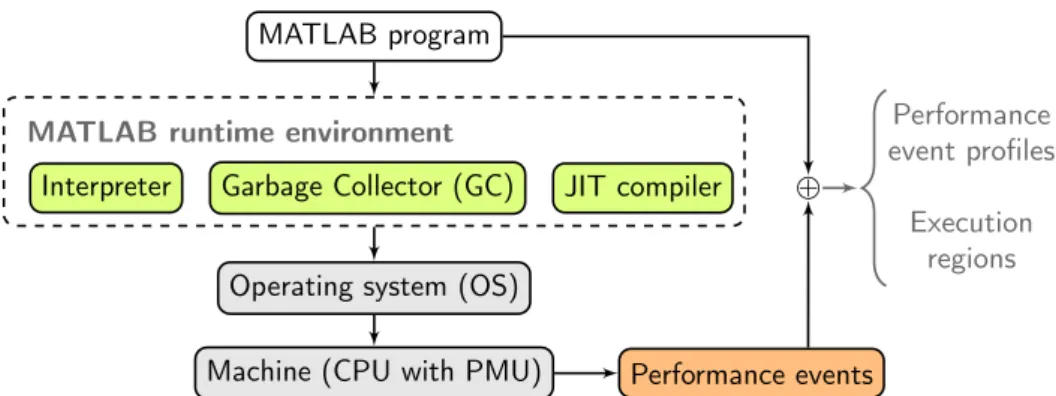
MATLAB environment consists of an interpreter, garbage collector, and Just-In-Time (JIT) compiler among others. However, these components are neither open-source nor documented. Therefore, the environment is a black-box which requires an entirely new approach for its analysis, as current performance modelling techniques aim mainly at open-source solutions. To address this challenge, we focus on the execution of MATLAB programs directly on the CPU. For this task, we use a well-known performance event profiles which measure how particular events on the CPU change over time, e.g. the number of cache misses or floating-point operations. Furthermore, we introduce a notion of execution regions which divides performance profiles into segments with particular properties, e.g. a data copy or a floating-point computation.

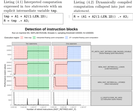
Using performance event profiles and execution regions, we have analysed how particular expressions are scheduled for the execution by the MATLAB JIT compiler. The compiler generates machine code for a batch of functions at a time, called an instruction block. Therefore, by observing the activity of an instruction cache on the CPU, we can track when each block starts and ends. An instruction block is either a set of combinable functions which coexist together or a single function requiring the whole instruction block for itself.

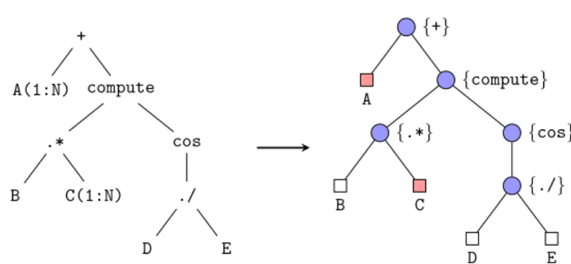
To predict the type and the order of instruction blocks, we have proposed a static tree-based model called the instruction tree. The model predicts, directly from the MATLAB code, what execution regions are generated while running the program. The instruction tree gives an insight into the execution of MATLAB programs, and it can be a basis for future performance models. Furthermore, with the knowledge gained from the analysis of the MATLAB environment, we have proposed several code transformations which create new optimisation opportunities. Repacking of array slices can increase the amount of JIT-compiled code in programs by performing array slicing before the actual computation, and range simplification, which reduces the number of redundant computation and indexing phases. Also, the proposed model indicates when the reordering, fusing and splitting of (sub-)expressions could increase the program performance as well.

The main contribution of this thesis is the methodology to analyse and discover how a black-box environment, such as MATLAB, executes programs. Furthermore, with the increased knowledge about the execution of programs, we have proposed several code transformations which can improve the per-formance of applications. During the work on the thesis, we have developed HU!M, a source-to-source compiler for MATLAB programs which performs automatic analyses and code transformations, and an interface mPAPI for accessing hardware performance counters directly from the MATLAB envi-ronment.

The creation of this thesis was an effect of superposition of various events and people met during my life. I am not exactly sure to whom I can attribute my appreciation and fascination of science, but whoever you are: well done! Firstly, I am grateful to my supervisors Corinne Ancourt, Claude Tadonki, and Jarosław Koźlak for their helpful, supportive, and encouraging guidance. This thesis is the result of our meetings and all tough questions asked during them. I have learnt a lot from you. Thank you.

CRI laboratory is a unique mix of science, friendship, and work, where time does fly a bit differently. I express my gratitude to past and present CRI members for creating this warm atmosphere and including me in the group: Maksim Berezov, Catherine Le Caër, Fabien Coelho, Laurent Daverio, Emilio Gallego, Florian Gouin, Pierre Guillou, Olfa Haggui, Olivier Hermant, François Irigoin, Pierre Jouvelot, Claire Medrala, Benoît Pin, Bruno Sguerra, Lucas Sguerra, Pierre Wargnier, and Katarzyna Węgrzyn-Wolska. I am indebted to François and Fabien for making my last year of studies possible.

I thank Michel Barreteau, François Giersh and Frédéric Barbaresco from THALES for their cooperation and an opportunity to prepare this thesis in the first place. Our meetings, although sparse, were always entertaining.

I say thanks to my dense friends: Jakub and Ziejka for always being there on-line; Panek for coming to us off-line; Adilla for all the voices; Gabriella for many topics to think about; Nathan for speed hiking; Laila for always having nuts; Tuanir for remembering the sound of bongos; Corinne for making Monika and me the happiest dog sitters of Orson on this side of the Seine; and the Chileans: Rocío, Estaban, and Hector for crossing our timelines.

Finally, I send love to my whole family for years of cheering, especially to my parents, Ewa and Arkadiusz, for all the support. I thank my sister Kinia and Leszek, for the best B&B in Warsaw. I am grateful to Monika’s parents, Małgorzata and Witold, for the help and time spent. At last, I send my love to Monika for not falling asleep while listening about MATLAB. You are, indeed, optimal.

1 Introduction 15 1.1 Motivation . . . 16 1.2 Research challenges . . . 18 1.3 Thesis contributions . . . 19 1.4 Thesis structure . . . 20 2 Related work 23 2.1 Acceleration of MATLAB programs . . . 24

2.1.1 Compilation of MATLAB programs . . . 24

2.1.2 Transformation of MATLAB code . . . 27

2.1.3 Alternative execution environments . . . 28

2.1.4 Analysis of MATLAB programs . . . 28

2.2 Performance analysis . . . 31

2.2.1 Metrics and models . . . 31

2.2.2 Hardware performance counters . . . 32

2.2.3 Profiling . . . 34

2.2.4 Performance of execution environments . . . 35

2.3 Conclusion . . . 35

3 Performance event profiles 37 3.1 Overview . . . 38

3.2 Motivation . . . 39

3.3 Building performance profiles . . . 41

3.3.1 Selecting the sampling event . . . 43

3.3.2 Selecting the sampling threshold . . . 45

3.3.3 Performance profiles with mPAPI . . . 48

3.4 Finding execution regions . . . 50

3.5 Case study: cost of array slicing . . . 52

3.6 Conclusion . . . 55

4 Execution model for MATLAB 57 4.1 Scope of the execution model . . . 58

4.2 Instruction blocks in JIT compilation . . . 59 7

4.3 Detecting instruction blocks . . . 61

4.4 JIT compilation of functions . . . 64

4.4.1 Built-in functions . . . 64

4.4.2 User-defined function . . . 66

4.5 Instruction tree . . . 68

4.5.1 Building minimal instruction tree . . . 69

4.5.2 Predicting execution from minimal instruction tree . . 72

4.6 Conclusion . . . 74

5 Code transformations for array operations 77 5.1 Redesigning array slicing . . . 78

5.1.1 Dynamic array slicing . . . 78

5.1.2 Eliminating redundant 0-initialisation . . . 79

5.2 Repacking of array slices . . . 82

5.3 Range simplification . . . 83

5.4 Profile-guided loop vectorisation . . . 86

5.5 Conclusion . . . 91 6 HU!M compiler 93 6.1 Overview . . . 94 6.2 Influences . . . 95 6.3 Code analysis . . . 97 6.4 Code transformation . . . 100 6.4.1 Loop vectorisation . . . 100

6.4.2 Fast array slicing substitution . . . 102

6.4.3 Repacking of array slices . . . 103

6.5 Conclusion . . . 103

7 Evaluation of the execution model and code transformations105 7.1 Evaluation of the execution model . . . 106

7.1.1 Model precision . . . 106

7.1.2 Splitting expressions . . . 106

7.1.3 Reordering operations . . . 108

7.1.4 Information limit of performance profiles . . . 110

7.2 Evaluation of the range simplification . . . 111

7.3 Evaluation of the repacking of arrays . . . 114

7.4 Conclusion . . . 116

8 Conclusion 119 8.1 Summary . . . 120

A Experiment methodology 125 A.1 Preparation of the environment. . . 125 A.2 Collecting measurements . . . 126 A.3 Machine specification . . . 126

B mPAPI 129

B.1 mPAPI interface. . . 130 B.1.1 Enumerating available performance events . . . 130 B.1.2 Measuring performance events in counting mode . . . 130 B.1.3 Measuring performance events in sampling mode . . . 131

C Menchi 133

C.1 Benchmark preparation . . . 134 C.2 Experiment specification . . . 135 C.3 Experiment modes . . . 136

1.1 Multiplication of random square matrices in C, MATLAB, and

Python . . . 16

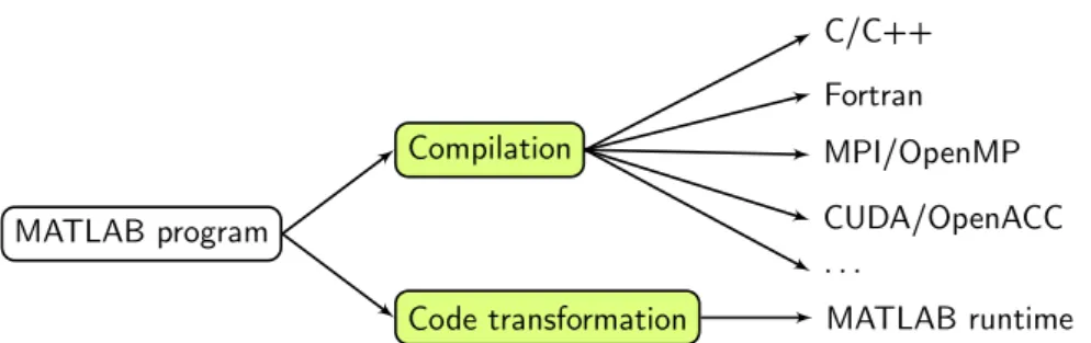
1.2 Improving performance of MATLAB . . . 17

3.1 Components of program execution in MATLAB . . . 38

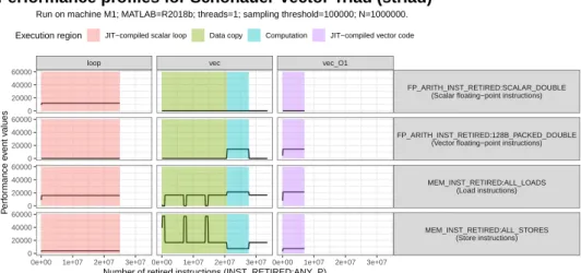
3.2 Performance event profiles for the striad kernel . . . 40

3.3 Performance profiles built using various sampling events . . . 44

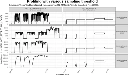
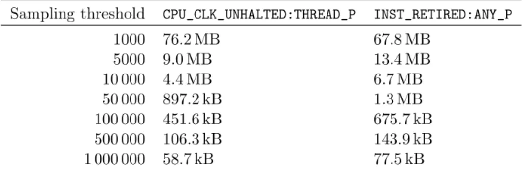
3.4 Performance profiles built using various sampling thresholds . 46 3.5 Impact of the sampling threshold on the duration of perfor-mance profiles . . . 47

3.6 Workflow of creating performance traces with mPAPI . . . 49

3.7 Cost of performing data copy during array slicing . . . 54

4.1 Components of MATLAB expressions with array operations . 58 4.2 Detection of instruction blocks with code examples . . . 63

4.3 Code examples for testing dynamic compilation of user-defined functions . . . 67

4.4 Step 1: Conversion of an expression to AST . . . 69

4.5 Step 2: Conversion from an AST to the instruction tree . . . 70

4.6 Step 3: Removal of array reference leaves . . . 70

4.7 Step 4: Merging of instruction blocks to form the minimal instruction tree . . . 72

4.8 Instruction chain obtained from the flattened instruction tree 74 4.9 Prediction of the execution regions and their order . . . 75

5.1 Zero initialisation in array slicing . . . 80

5.2 Results of applying repacking of array slices . . . 84

5.3 Performance profiles of array slicing with ranges . . . 85

5.4 Profiling of loop vectorisation . . . 88

5.5 Results of profile-guided vectorisation . . . 90

6.1 Overview of analyses in HU!M . . . 97

6.2 Hierarchy of classes representing the instruction tree . . . 97

6.3 Overview of transformations in HU!M . . . 100 11

6.4 Fast array slicing substitution in HU!M . . . 102

6.5 Repacking of array slices in HU!M . . . 103

7.1 Execution regions of MIT-2 example . . . 107

7.2 Example of splitting an expression into sub-expressions . . . . 108

7.3 Splitting expression to perform vector operations . . . 109

7.4 Minimal instruction tree after reordering of instructions . . . 109

7.5 Reordering expression to reduce instruction blocks . . . 110

7.6 Execution regions of MIT-1 example . . . 111

7.8 Performance profiles of array slicing with ranges . . . 113

7.9 Execution time of range simplification . . . 114

7.10 Repacking of array slices on Livermore kernels . . . 115

7.11 Repacking of array slices on LCPC16 kernels . . . 117

A.1 Hierarchical topology of test machines . . . 127

C.1 Workflow of code benchmarking with Menchi . . . 133

D.1 Optimised loop crni2 from Chen et al. [1] . . . 141

D.1 Optimised loopsnw2and nw3from Chen et al. [1] . . . 142

D.1 Optimised loop fft1 from Chen et al. [1] . . . 143

D.2 Extended version: cost of performing data copy during array slicing . . . 144

D.3 Execution regions of MIT-3 example . . . 145

D.4 Execution regions of MIT-4 example . . . 145

D.5 Execution regions of MIT-5 example . . . 146

D.6 Execution regions of MIT-6 example . . . 146

D.7 Execution regions of MIT-7 example . . . 147

2.1 List of research and industrial compilers for MATLAB. . . 25 3.1 Size of profile files with changing sampling threshold . . . 48 3.2 Selected programs for the analysis of data copy cost . . . 53 4.1 Performance event candidates for the detection of instruction

blocks . . . 62 4.2 Test codes used for the detection of dynamic compilation . . . 65 4.3 List of single and combinable built-in functions . . . 66 4.4 Examples of expressions with their minimal instruction trees . 73 5.1 Experiment reproduction of vectorisation by Chen et al. [1] . 87 5.2 Results of loop profiling for profitable loop vectorisation . . . 89 7.1 Machine instructions counted by theFP_ARITH_INST_RETIRED:*

family of performance events on Skylake and Coffee Lake microarchitectures. . . 112 A.1 Specification of test machines . . . 126 C.1 Benchmark specification generated by CodeExtractor . . . . 135 C.2 Experiment modes in Menchi tool . . . 137

Introduction

Résumé

Pour de nombreux chercheurs et programmeurs, MATLAB est un outil pratique pour le prototypage rapide de solutions à des problèmes de calculs complexes, car le langage possède une syntaxe claire et une vaste bibliothèque de fonctions et d’algorithmes intégrés. Bien que les versions récentes de MATLAB soient compilées en temps réel (JIT), ses performances sont souvent inférieures à celles d’autres langages tels que le C, Fortran et même Python. Auparavant, les chercheurs ont adopté deux approches pour améliorer les performances des programmes MATLAB : 1) la compilation du code MATLAB comme celle des langages C et Fortran, et 2) la transformation du code des programmes MATLAB pour utiliser des constructions de langage plus rapides. Alors que 1) la compilation ignore entièrement l’environnement d’exécution de MATLAB, 2) la transformation du code ne fonctionne bien que lorsque nous savons précisément comment MATLAB exécute les programmes. Dans cette thèse, nous présentons une analyse de performance permettant de découvrir comment les applications s’exécutent dans l’environnement MATLAB. De plus, nous formalisons l’exécution des programmes avec un modèle d’exécution basé uniquement sur les arbres permettant d’effectuer de nouvelles transformations de code qui augmentent les performances des programmes MATLAB compilés en temps réel (JIT). Nous avons également développé plusieurs outils et un compilateur qui facilite l’utilisation de l’analyse des performances et l’application des transformations de code.

Introduction

For many programmers and researchers, MATLAB is an everyday tool, ca-pable of expressing even the most complex computational problems in an easy, concise, and interactive way using its dynamic execution environment. MATLAB achieves this by mastering the idea of programming language as mathematical notation, first proposed by Iverson [2] in his APL language. Consequently, MATLAB is a domain-specific language dedicated to linear algebra and array-based computations. Moreover, in the language, vectors,

1 // C language

2 double _*randmatmul(int n) {

3 double _{*A = myrand(n*n);}

4 double _{*B = myrand(n*n);}

5 double _{*C = (}double_*)

6 _malloc(n*n*sizeof(double));

7 cblas_dgemm(CblasColMajor, CblasNoTrans, CblasNoTrans, n, n, n, 1.0, A, n, B, n, 0.0, C, n); 8 free(A); 9 free(B); 10 return C; 11 } 1 # Python + NumPy 2 import numpy as np; 3 def randmatmul(n): 4 A = np.random.rand(n,n) 5 B = np.random.rand(n,n) 6 return np.matmul(A,B) 1 % MATLAB 2 function C = randmatmul(n) 3 A = rand(n,n); 4 B = rand(n,n); 5 C = A * B; 6 end

Figure 1.1: Code examples for the multiplication of random square matrices written in three different languages: C, MATLAB, and Python (from Julia Microbenchmarks [3]). C code requires manual memory management, an explicit call to the external BLAS routine, and type declarations.

matrices and multi-dimensional arrays are first-class citizens with dedicated operations. Thus, expressing computations using these multi-element struc-tures is as easy as working with scalar variables in any other language.

MATLAB is not only a programming language, it is a problem-solving environment [4], with more than 2900 built-in functions, 53 specialised tool-boxes, 8 compilers, and 1 code profiler (as of version R2019b). Figure 1.1 compares multiplication of random square matrices written in C, Python, and MATLAB. While the code of Python with NumPy library is fairly similar to the MATLAB code, the C code requires an implementation of functionmyrand

for random generation of arrays (MATLAB hasrand); a call to the external

dgemmBLAS routine for matrix multiplication (MATLAB uses Intel MKL [5]

for*operator seamlessly); a manual memory management using malloc and free (MATLAB performs automatic memory [de]allocation); and explicit

declarations of typedouble(MATLAB works on doubletype by default, also

it has dynamic and weak type system). The inherent easiness of writing code together with the numerical orientation make MATLAB especially suitable for fast prototyping of applications in computational science and engineering (CSE), signal processing, control systems, image processing, machine learning,

and many more disciplines.

1.1

Motivation

The interactive and dynamic natures of MATLAB, so desirable for fast prototyping, required MATLAB programs to be interpreted at first in 1984 [6], and then gradually moved to more powerful techniques such as program

MATLAB program Compilation Code transformation C/C++ Fortran MPI/OpenMP CUDA/OpenACC . . . MATLAB runtime

Figure 1.2: Two possible approaches to improving performance of MATLAB programs.

execution using bytecode-based virtual machine (VM) [7] and Just-In-Time (JIT) compilation [8]. In order to stay relevant and increase its performance, over the years, MATLAB received support for vector instructions around year 2000 [9], included Just-In-Time (JIT) compiler in 2002 with MATLAB 6.5, introduced explicit parallelism with Parallel Computing Toolbox in 2004, executes built-in functions on many-threads since R2007b, included computation on Graphics Processing Unit (GPU) in R2010b, and finally, obtained new execution engine (LXE) in R2015b [10] which combines the interpreter and the JIT compiler under a single monolithic architecture.

Unfortunately, the JIT compilation induces additional costs related to the runtime preparation of the code just before the execution. In order to compete with statically compiled languages like C and Fortran, the JIT compiler must be as good, or even better, as compilers for those languages. Therefore, since the beginning of MATLAB, researchers and companies have worked on methods and tools for optimising MATLAB programs [1,11–21]. Figure 1.2 presents two common approaches to improving MATLAB performance: (1) compilation and (2) code transformation. Other techniques include, e.g. developing new virtual (VM) machines [22], JIT compilers [23], and parallel extensions [24, 25]. From the previous works, the MATLAB translation to C and Fortran are, by far, the most popular approaches, probably because they bypass performance limitations of the MATLAB runtime whatsoever. Instead, the compilation can benefit from years of research on optimising compilers [26–28]. However, compilation of MATLAB programs breaks the fast prototyping development cycle. Imagine our problem is compute-intensive and it requires compilation before each run. In such case, we need to leave the MATLAB environment and switch to other compilation toolchain. Therefore, in order to facilitate program development, we have focused on source-to-source transformations of MATLAB programs. Moreover, code transformations for MATLAB were much less investigated by researchers than MATLAB compilation, and as such, we believe there is still room for improvement.

1.2

Research challenges

Researchers have applied code transformations to MATLAB since the 1990s starting with the FALCON project [29, 30]. Around year 2000, the huge benefit of loop vectorisation made it a primary code optimisation technique for MATLAB programmers. Since then, researchers applied vectorisation automatically to MATLAB programs [9, 21]. However, because of the im-provements to JIT compilation in MATLAB, the systematic vectorisation of every loop is no longer a viable approach [1, 31]. Therefore, the successful application of loop vectorisation and any other code transformation requires the understanding of how exactly MATLAB executes programs and a careful consideration of when and what transformation to apply.

MATLAB is a closed source, proprietary environment. Thus, programmers and researchers have almost no details from the vendor about how MATLAB really works. Moreover, the MATLAB language is dynamic with a weak type system which is not the best input for static code analysis, because of the lack of many information about the source code. This situation leads to the need of developing new approaches of characterising program execution and MATLAB itself. For this task, we have previously worked on several research directions, unfortunately with no positive results apart from gaining new knowledge.

Static heuristics for loop vectorisation. Our first approach to improv-ing performance of MATLAB programs was to create heuristics for checkimprov-ing when to apply loop vectorisation. In order to find key elements of programs contributing the most to the performance of loop vectorisation, we have used several performance models, analyses and metrics such as the Roofline Model [32], Top-Down Microarchitectural Analysis [33], cache and data reuse models, monitoring of hardware performance counters in the counting mode. However, every tested approach gave us only a global view on the program execution without any consideration for time-varying behaviour, which turned out to be a key factor. The lack of results from this approach lead us to a direction of profile-guided vectorisation using a simple profiling scheme described in Section 5.4 and [31]. Although, very useful and powerful, profile-guided vectorisation is not a solution to the initial goal of having static heuristics.

Machine Learning model for selecting loop vectorisation. Our next approach to the previous problem was based on Machine Learning for building a decision model for loop vectorisation. For this task, we have examined two approaches with vastly different representations of MATLAB programs. The work of Cavazos et al. [34] uses a vector of values from hardware performance counters to encode a single code example. Later, in order to predict if a loop is worth vectorising, we just run the loop and collect performance counters

which were then feed to the model. In contrast, the work of Cummins et al. [35] uses fully static representation, the string of the code example encoded using techniques used also in Natural Language Processing (NLP). Although, using the approach by Cavazos et al. [34] we were able to create promising models with high precision, we failed too find in them any important insights.

Warm-up state of JIT compiler in MATLAB. In this analysis, we have focused on the JIT compiler entirely and followed a study of Barrett et al. [36] about characterising warm-up stages of popular virtual machines (VM), e.g. HHVM [37], Graal [38], HotSpot JVM [39], and others. In the study, various benchmarks were repeatedly executed on each virtual machine to see when the JIT compilation happens and how it affects the performance. In MATLAB, we have observed that JIT compilation usually increases the program performance, however, in very rare cases it might even lead to performance degradation. Moreover, we have observe the JIT compilation happens during the first run of a program, which indicates that the JIT compiler in MATLAB has a single-tier policy [40].

All abovementioned challenges have only emphasized the need for a different approach to analyse, model, and understand how MATLAB executes programs, before working on code transformations for them.

1.3

Thesis contributions

In the thesis, we have focused on the development of new analyses and code transformations for MATLAB programs. The main contributions are built around three research questions:

• RQ1: Can we analyse and model how MATLAB works seen as a black-box?

• RQ2: Are we able to propose new code transformations for MATLAB? • RQ3: Is it possible to improve MATLAB performance without breaking

much the fast prototyping cycle?

Analysis and modelling. The answer to question RQ1 is divided into two Chapters 3 and 4. In Chapter 3, we introduce performance event profiles (PEP) which are an inventive use of hardware performance counters to analyse time-varying aspects of the program execution. Later, in Chapter 4, we use the profiles to discover and build an execution model for MATLAB expressions. The model is encoded as instruction trees where each node represents a block of instructions executed together by the JIT compiler. Moreover, connections between these nodes indicate their execution order. The result of the model is a prediction of how MATLAB executes a given expression.

New code transformations. To answer the next question, RQ2, we use the combined results of Chapters 3 and 4 to propose several specialised code transformations for MATLAB programs, e.g. repacking of array slices and range simplification in Chapter 5. For example, the repacking leverages the fact that JIT compiler in MATLAB prefers expressions without indexed variables, because then the expressions can be compiled as one block of instructions. Therefore, the repacking extracts and substitutes indexed variables with references to temporary arrays. Furthermore, in Section 5.4, we take a fresh look on loop vectorisation applied to MATLAB programs in the profile-guided context.

Fast prototyping cycle. The last question RQ3 is answered indirectly with the knowledge from previous answers and the content of Chapter 6. The chapter presents our HU!M compiler which implements presented execution model and code transformations. These transformations not only keep the similar level of code readability, but also once applied, they persist in the code without future need to reapply them again, as opposed to MATLAB compilation which works on the whole compilation unit (usually a function) and requires recompilation even after small change in the source code. Moreover, the majority of presented code transformations (except for loop vectorisation) requires little to none of code analysis, while other, e.g. dynamic array slicing, postpone the analysis until the runtime.

1.4

Thesis structure

In Chapter 2, we outline collection of works related to three topics: (1) acceleration of MATLAB programs; (2) performance analysis of computer programs; and (3) analysis of runtime environments. The topic (1) shows the scale of the research that went into the optimisation of MATLAB programs. Moreover, topics (2) and (3) show other attempts to understand the behaviour of program execution and runtime environments, e.g. Python and JVM.

The next three Chapters 3 to 5 describe our contributions:

• Performance event profiles (PEP) are an inventive way to use perfor-mance profiles built using hardware perforperfor-mance counters to discover and understand the program execution (Chapter 3). Every performance profile consists of several execution regions, each depicting different kind of a computation. Furthermore, we present how to create performance profiles using our open source tool mPAPI.

• Execution model of MATLAB expressions is encoded as an instruction tree which groups instructions into blocks (Chapter 4). Each instruction block is separately compiled for the execution by the JIT compiler. Using our model, we are able to predict the order of instruction blocks and

their content, by tracking which instructions merge together in the process of obtaining the minimal instruction tree.

• Dynamic array slicing, repacking of array slices, range simplifications are code transformations for MATLAB programs introduced in Chapter 5. They improve performance of MATLAB expressions without impacting drastically the code readability. Moreover, in Chapter 5, we have analysed loop vectorisation applied with profiling information.

In Chapter 6, we present our source-to-source compiler HU!M capable of applying transformations from Chapter 5 in an automatic manner. Moreover, the compiler implements our execution model from Chapter 4, and it is capable of giving prediction about the program execution directly from an input source code. Finally, Chapter 8 summarises the research tasks performed during the work on the thesis, obtained results, and the future work.

The thesis consists of 4 appendix with descriptions of experiment method-ology, our two tools mPAPI and Menchi, and a collection of additional results. Appendix A describes the experiment methodology used for every results (plots included) in the thesis, except for the experiments in Section 5.4. The goal of the methodology is to limit measurement errors and non-deterministic events as much as possible, and to correctly summarise the obtained mea-surements, e.g. using confidence intervals [36,41,42]. Moreover, Appendix A contains a list of two machines used in our experiments.

Appendix B describes mPAPI which is a MATLAB interface for accessing hardware performance counters built on top of the PAPI library [43]. The interface extends the capabilities of the official PAPI interface for MATLAB with collecting performance counters in the sampling and the multiplexed modes, and allowing to measure counters for separate threads.

In Appendix C, we describe Menchi, an experiment generator tool which was used to prepare each test in the thesis in a single and consistent manner.

Finally, Appendix D contains additional codes and plots which could not fit into the main part of the manuscript.

Related work

Résumé

Dans ce chapitre, nous nous sommes concentrés sur les travaux de recherche liés à l’accélération des programmes MATLAB et à l’analyse des performances des applications. Bien qu’il existe plusieurs autres domaines de recherche proches des travaux présentés dans cette thèse, ces deux sujets sont les plus importants.

Au fil des ans, les chercheurs ont créé plusieurs compilateurs de MATLAB vers d’autres langages : FALCON, Otter, Match, MATISSE, ou le codeur officiel de MATLAB, pour n’en citer que quelques-uns. Aujourd’hui, seul MATLAB Coder est prêt à être utilisé par les programmeurs et les scientifiques, mais le processus d’utilisation n’est pas entièrement automatisé. D’autre part, la recherche sur les

transformations de code des programmes MATLAB est très rare. Pendant de

nombreuses années, le savoir collectif pour augmenter les performances a inclus la vectorisation des boucles dans les codes MATLAB. Cependant, les compilateurs récents de MATLAB peuvent produire un code plus rapide sans vectorisation. La simple décision de vectoriser une boucle ne peut être prise qu’avec l’aide de modèles d’exécution qui ont été étudiés auparavant dans le contexte de MATLAB.

Pour créer un modèle d’exécution et un modèle de performance, nous devons utiliser des techniques d’analyse de performance. Les mesures et modèles de perfor-mance classiques, tels que le nombre d’instructions par cycle (IPC) ou le modèle de cache d’exécution (ECM), soit ne prennent pas en compte le comportement variable dans le temps des programmes analysés, soit ne décrivent qu’une perspective abstraite de l’exécution du programme. Les compteurs de performance matérielle donnent une vue détaillée de l’exécution du programme car ils représentent la façon dont une unité centrale exécute le programme. De plus, les valeurs des compteurs de perfor-mance peuvent être échantillonnées dans le temps, donnant ainsi une description de l’exécution du programme qui varie dans le temps. La majorité des analyses de performance ont été appliquées à des langages et des environnements d’exécution de logiciels libres, par opposition aux boîtes noires de logiciels propriétaires comme MATLAB.

Introduction

The work presented in the thesis, spans across several important topics: programming languages, compiler construction, performance analysis, design of processors, code transformations, compilation, to name a few. For this chapter, we have selected two most important topics connected to our work: (1) acceleration of MATLAB programs; (2) performance analysis of computer

programs and runtime environments.

2.1

Acceleration of MATLAB programs

Acceleration of MATLAB programs has a long history full of many research and industrial projects. In this section, we describe four major components of improving MATLAB programs: (1) compilation; (2) transformation; (3) development of new virtual machines and parallel extensions; and (4) analysis.

2.1.1 Compilation of MATLAB programs

Compilation of MATLAB programs, especially to static languages like C or Fortran, brings the results of many research works devoted to loop transfor-mations and optimising compilers for these languages. Moreover, because the input language is MATLAB, programmers still benefit from MATLAB language clarity and fast prototyping properties. Furthermore, compilation of MATLAB is a solution for porting programs to parallel and heterogeneous computing platforms.

Unfortunately, not all MATLAB built-in functions are supported by MATLAB compilers. Even today, the official MATLAB to C compiler, MATLAB Coder, supports the majority but not all built-in functions [44]. Moreover, other MATLAB compilers support only a handful of built-ins. Although, the compilation of MATLAB programs is common and beneficial, it is not always applicable. However, some compilers port a MATLAB program onto a new platform which does not run MATLAB environment. A good example is the MATISSE compiler which targets embedded systems [45] and heterogeneous computing platforms with OpenCL [46], otherwise not available for MATLAB programs.

In this section, we present various compilers for MATLAB language depicted in Table 2.1. Moreover, we briefly describe some of them in the subsequent paragraphs to illustrate the variety of targeted languages and architectures. However, we do not focus on their code analysis capabilities, leaving this part for the Section 2.1.4.

FALCON. FALCON is a programming infrastructure for creating numeric applications using MATLAB language [48]. The tool is able to transform MATLAB code, as well as compiled it to Fortran 90. FALCON infers

Table 2. 1: List of researc h and industrial compi lers for MA T LAB. Compiler A ctiv e years Target language Platform Ref FALCON 1995-2001 Fortran/MA TLAB C P U [11, 47, 48] Otter 1998-1 999 C/MPI CPU [12, 49] Menhir 1998-19 99 C/F ortran C P U [19, 50] MA TCH 1999-2003 VHD L FPGA/DSP chips [51–53] Mat2C 2006-2007 C CPU [54] OMPC 2009–2010 Python CPU [55] MEGHA 2011–2012 C++/CUD A CPU/GPU [56] MA TISSE 2013–2017 C/Op enCL Em bedded/Heterog eneous [13] Mc2F or 2013–2014 Fortran95 CPU [15] eV ariX/COLD 2013–2018 C CPU/Heterogeneous [57] Mix10 2014 X10 CPU [16] m2cpp 2015–20 18 C++ CPU [5 8, 59] StencilP aC 2016 C/Op enMP/MPI/Op enA CC CPU/GPGPU [60] MatJuice 2016 Ja vaScri pt CPU [61] Latifis et al. 2017 C/S IMD E m bedded/System-on-Chip (SoC) [6 2]

several information about variables in programs, such as their type, shape, size of each dimensions, and their structural properties, e.g. if a matrix is diagonal or triangular. The structural analysis is used to generate specialised arithmetic operations which work especially well on matrices with particular properties [11]. Furthermore, the analyses can be static (working from the source code) or dynamic (deferred to the runtime). For the analyses, FALCON represents MATLAB programs in the Static Single Assignment (SSA) form.

Moreover, FALCON is capable of transforming MATLAB programs to achieve better performance. However, the code transformation is manual and requires inserting annotations into the code. Further, the annotated code is transformed accordingly to one of the patterns in a database of rewriting rules. The rules include algebraic restructuring such as reordering matrices during multiplication, and primitive-set translation like loop interchange [11].

Otter. Otter is a compiler which not only translates MATLAB into C, but it also parallelises the code using Message Passing Interface (MPI) [49] and delegates numerical computations to parallel implementation of the Linear Algebra PACKage (LAPACK) library called Scalable LAPACK (ScaLAPACK) [12]. The compiler uses Static Single Assignment (SSA) as

intermediate representation of MATLAB programs.

MATCH. MATCH is a compiler targeting heterogeneous platforms such as Digital Signal Processing (DSP) chips and FPGA. The compiler has a very detailed parser for the MATLAB language which development was detailed in an extensive report [63,64].

Mat2C. Joisha and Banerjee, after years of work on shape inference for MATLAB [17,65], have created MATLAB to C compiler called Mat2C. The compiler uses MAGICA, their shape inference engine.

MATISSE. MATISSE is a compiler from MATLAB language to C and OpenCL [13, 66], focusing also on embedded systems [45]. MATISSE uses aspect-oriented programming language called LARA [67] to specify missing information required for the compilation. LARA allows to declare, e.g. data types and shapes, which are dynamic information in MATLAB and usually unspecified in the MATLAB source code.

m2cpp. m2cpp1 _{is a MATLAB to C++ compiler which generates parallel}

code using OpenMP [68] or Intel TBB [69] libraries. Moreover, for the computations, m2cpp utilizes Armadilo library. The compiler uses external file with meta-information such as types and shapes of variables required for the compilation.

1

2.1.2 Transformation of MATLAB code

Although, much less popular, the code transformation of MATLAB programs was investigated by researchers as well. The biggest disadvantage of this approach is that the final gain from optimisation is limited to the performance of the MATLAB environment.

Loop vectorisation

Still today, loop vectorisation is considered as a primary tool for increasing performance of MATLAB loops2_{. Menon and Pingali [9] have implemented}

automatic loop vectorisation in FALCON [11]. Moreover, they have performed one of the first studies on the effectiveness of loop vectorisation. Their results have shown that vectorisation is always beneficial and can be applied systematically.

Two further works on automatic loop vectorisation are mainly concern about shape analysis and the validity of the vectorisation. Birkbeck et al. [21] introduced the notion of dimensionality abstraction which helps to check if the code after vectorisation is correct. If not, their vectoriser can transpose arrays and check if this transformation made the code correct. Moreover, their vectoriser includes a database of common patter used in loop vectorisation. The next study by Chen et al. [1] improved on the idea of dimensionality abstraction by introducing a data-flow analysis called promoted shape. The analysis was implemented in their vectoriser Mc2Mce3 _{along with automatic}

shape inference built on top of the Tamer [1, 70]. With the analysis, au-thors were able to perform loop vectorisation, but also vectorisation of the whole user-defined functions (also called procedure vectorisation [20]). Both presented approaches uses the same vectorisation algorithm by Allen and Kennedy [71,72] as their base. However, both Chen et al. [1] and Birkbeck et al. [21] are not considering when vectorisation might not be beneficial, applying it only systematically.

Arithmetic simplification

Often, mathematical equations can be simplified and optimised. The same is true for MATLAB code which expresses these equations. In FALCON compiler, using annotations, it is possible to perform algebraic restructuring, such as reordering of matrices during multiplication, in order to reduce the number of performed arithmetic operations [11].

Menon and Pingali [73] introduced a whole framework for restructuring expressions called Abstract Matrix Form (AMF). AMF is an algebraic lan-guage for expressing semantics and transformations of element-wise matrix

2

https://www.mathworks.com/help/matlab/matlab_prog/vectorization.html 3

operations. Moreover, the framework contains several rewriting rules for simplifying computations which result in significant performance gain [9,73].

Partial evaluation

Elphick et al. [74] presented a partial evaluation system for MATLAB where rarely (or never) changing parts of the programs are evaluated before the actual execution. In other words, partial evaluation is about evaluating static instructions and leaving dynamic instructions for later. The presented results were optimistic, however, their system considered only a small subset of MATLAB language.

2.1.3 Alternative execution environments

During the efforts to increase MATLAB performance, there were several attempts to build an alternative to the MATLAB environment.

MaJIC. Almási and Padua [18, 23] have built a Just-In-Time compiler for MATLAB using the FALCON infrastructure [11]. The compiler performs dynamic type, shape, and range analyses right before the code execution. Moreover, MaJIC reduces the amount of required temporary variables, auto-matically preallocates them, unrolls vector operations on small arrays, and performs preallocation for arrays which change their size during execution.

McMV. Chevalier-Boisvert et al. [22] have presented a new virtual machine (VM) for MATLAB with a JIT compiler. The JIT compiler is built using LLVM infrastructure [75], but it also has a mark-and-Sweep garbage collector and integration with numerical libraries: ATLAS, BLAS, LAPACK. Further-more, the JIT compiler performs on-the-fly specialisation and optimisation of functions based on the type of their arguments. The compiled functions are later versioned and kept in a database for further function calls.

MATCH Virtual Machine (MVM). Haldar et al. [76], using an infras-tructure of the MATCH compiler, have built a virtual machine for MATLAB language. The machine is capable of generating parallel code at runtime, thus, solving problems of having insufficient information about types and shapes of variables. Moreover, MVM executes parallel tasks in an out-of-order model to better exploit available resources.

2.1.4 Analysis of MATLAB programs

The analysis of MATLAB programs can be divided into three main categories: kind, shape, and type analysis. While the shape and type analyses are common for other languages and environments, kind analysis is unique to

MATLAB and results from two issues: (1) dynamic nature of the language where the same label can point to different objects in the course of the program execution; and (2) the ambiguity in the language syntax where the same expressionidentifier() could point to a function call or an array slice,

two vastly different entities.

In our work, we use only a very simplified kind analysis based on the database of built-in functions, and dimensionality based shape analysis proposed by [21]. Moreover, when comes to types, we consider only double

type representing double-precision floating point numbers.

Kind analysis

The goal of kind analysis is to statically determine if a label points to: a

function call, variable or a package name. During the program execution, kind analysis is easily resolved with exist label function which not only

tests the existence of thelabelin the workspace, but it also returns thelabel

type (e.g. variable, function, MEX-file, class). However, the source code of MATLAB program obviously lacks this information, especially because the content of thelabel can dynamically change during the program execution.

The name kind analysis for this problem, along with a detailed semantics of how MATLAB 7 (year 2004) resolves this problem was described by Doherty et al. [77]. Moreover, Doherty et al. have created an algorithm to perform kind analysis using, e.g. flow-sensitive information. While previous works have performed kind analysis as well, most notably in FALCON [48], Menhir [19,50], and MATCH [63,64], they did not call it this way. Usually, their approach was to mark an identifier as a function if the identifier was in a database of built-in functions or when an inter-procedural analysis of user-defined functions has found a corresponding function definition. Otherwise, depending on the reaching definition, the label was deemed as a variable.

Shape analysis

In the world of array programming languages, shape analysis concerns with the size of multi-dimensional arrays, their rank (number of dimensions), and how their size changes after performing operations on them. As opposed to shape analysis in imperative languages like C, where compilers analyse properties of heap-allocated data structures, e.g. linked lists [78].

Lattice-based approach. The most common shape analysis for MATLAB, used in e.g. FALCON [48], Menhir [19], or McJIC [18], is based on a lattice defining a hierarchy of shapes (e.g. row vector, matrix, unknown) with rules for resolving shape when arrays are used as arguments to MATLAB functions. However, these analyses were always limited to matrices and, in many cases, they return anunknownshape, due to a lack of required shape information.

Algebraic approach. A completely other algebraic approach was pre-sented by Joisha and Banerjee [17]. Their methodology expresses the shape of each variable as an algebraic expression. If a dimension or array rank is unknown, it is represented as a free variable in the equation. Therefore, the method instead of returning anunknown value, always returns an equation

expression of the shape, even when parametrised with variables. The method with a dedicated inference engine called MAGICA [79] was implemented in Mathematica [80, 81]. The method is powerful, however, it is not only complicated, but also not very useful in many contexts, such as static code generation because the parametrised formulas with missing values are un-acceptable for compilation, and they need to be resolved during the code generation phase. Nevertheless, the analysis was used in compiler Mat2C [54], built by the authors of MAGICA [79].

Dimensionality analysis. Introduced by Birkbeck et al. [21], dimension-ality analysis is an example of specialised shape analysis performed only in the context of automatic loop vectorisation. This analysis has two goals: (1) to validate if the vectorisation was correct, and (2) to transpose arrays so that their shapes are compatible. Therefore, the analysis can be simple and not concerned about the exact size for each dimension. Dimensionality of arrays is represented using only three values1, *and ri to indicate the

dimension of size equals to 1, more than 1, or having a value obtained after a loop was vectorised along the i-th dimension, respectively. For example, this system represents a scalar as(1, 1), a row vector as(1, *), a column vector

as(*, 1), and a matrix (*, *). However, this shape information must be

manually inserted using directives and could not be inferred automatically.

Promoted shape. Demonstrated by Chen et al. [1], promoted shape is also a dedicated analysis to loop vectorisation. However, the analysis extends the concept of dimensionality analysis [21] to user-defined functions, and using data-flow techniques, to flow-sensitive code. Moreover, the implementation of the analysis inside the vectoriser Mc2Mc uses value analysis from Tamer [70], which can statically infer the exact shape of an array, if only possible. Therefore, in many cases there is no need for explicit directives with shape information like in the dimensionality analysis by Birkbeck et al. [21].

Type analysis

Some compilers had no type inference, instead, they incorporate a set of directives for specifying the types, shapes, and other information. For example in the work of Ramaswamy et al. [82], the presented compiler accepts directives e.g. %! local float fool(128,128); for type and shape. Other compilers have simple algebraic or lattice-based type inference like the work by Latifis et al. [62]. Similarly, FALCON implements a SSA-based forward propagation

inference algorithm [11, 47, 48]. In FALCON, if a type inference yield an unknown type, then the compiler generates code for dynamic type inference which is performed at runtime.

Domain-Specific Language (DSL) for type propagation. Type anal-ysis is not only about inference rules because, with a vast number of built-in functions, it is hard to track and collect type information for them. For this problem, Dubrau and Hendren [70] have prepared a domain specific language for expressing how types propagate and change from the arguments of a built-in function to the result of the function.

2.2

Performance analysis

Precise performance analysis of computer system, at current state, is extremely complex which Abel and Reineke have recently summarised [83]:

“Modern microarchitectures are some of the world’s most complex man-made systems. As a consequence, it is increasingly difficult to predict, explain, let alone optimize the performance of software running on such microarchitectures. As a basis for performance predictions and optimizations, we would need faithful models of their behaviour, which are, unfortunately, seldom available.”

In this section, we describe several means to analyse and express perfor-mance of applications, without having an accurate model of the processor.

2.2.1 Metrics and models

When faced with hard problems, researchers delve into abstractions and simplifications. One example of such simplifications is performance metrics which describes one (or several) aspect of the program execution. Common metrics include: instructions per cycles (IPC) [84], loop balance [85], data reuse [86], etc. Metrics can be divided into dynamic and static, the former come as a result of measurements, while the latter are built just from analysing the program source code. Nevertheless, these metrics describe only small parts of the program execution like cache memory system, or utilisation of execution units in processor.

To get a more global view, we can use models such as polyhedral model [26], Roofline Model [32,87–89], or Execution-Cache-Memory (ECM) [90]. These models are specialised in expressing how well the program will execute or what is the execution bottleneck. Nevertheless, each of them is only a part of the story, e.g. Roofline Model focuses on memory bandwidth (or caches in other available extensions); polyhedral model focuses on the order of memory access and computations.

Researchers also have created metrics dedicated to virtual machines, e.g. for JVM, however, these metrics mainly consider properties of the bytecode, and not the virtual machine directly. Consequently, none of these metrics and models are useful for MATLAB because of three reasons: (1) their target is the machine; (2) MATLAB is a runtime environment which needs to be modelled on its own; and (3) MATLAB is a closed source tool.

2.2.2 Hardware performance counters

Different approaches to performance analysis are based on pure measurements using for example hardware performance counters. These counters are special purpose registers on processors which collect information about program execution in form of performance events, e.g. amount of cache misses, pro-cessor stalls [91]. Although, at first, the set of performance counters was ever changing and unstable, recently the available performance events stabilised with the introduction of architectural events which are available in the whole line of the microarchitectures. Accordingly to Stéphane Eranian [92], the Intel’s attitude towards performance counters has changed with the Intel Itanium processors. The second change can be observed with the introduction of Top-Down Microarchitecture Analysis (TMA) by Yasin [33]. TMA allows to find bottlenecks during program execution and to pinpoint them to a specific part of processor pipeline like the frontend, back-end, or execution units. Nowadays, performance counters are used in performance and power analyses, adaptive optimisations and many others.

Collecting performance counters. The popularity of performance coun-ters is backed by the number of tools and libraries allowing easy access to them. A few solutions include: OProfile [93], perfmon2 [94], PAPI [43, 95], Tiptop [96–98]. Moreover, some applications for performance analysis allow to collect performance counters as well. Intel® VTune [99] collects performance events to perform the Top-Down Microarchitecture Analysis (TMA). However, the measurements come only from one run of the application and they are multiplexed. Therefore, TMA analysis is not usable for short programs or programs with time-varying behaviour.

In our work, we use PAPI library which already has an interface to interact with MATLAB. However, we only reuse the interface and extend it with new functionalities collected inside mPAPI (see Appendix B).

Accuracy of performance counters There is still an ongoing debate about the precision and accuracy of performance counters which might differ depending on the microarchitecture, implementation of the code responsible for accessing performance counters in the kernel, acquisition methods and libraries, among others. Weaver et al. performed several studies on the topic [100,101]. General finding states there is usually a subset of accurate

and deterministic counters. However, the tests need to be performed for each new machine and its configuration [102]. In our work, we do not analyse the precision of performance counters, and instead, we only acknowledge their inherent imprecision for solving our problem of understanding the behaviour of MATLAB programs execution.

Feedback-directed optimisations. Schneider et al. [103] used perfor-mance events about cache activity to guide the Just-In-Time (JIT) compi-lation process. This type of optimisations is known as Feedback-Directed Optimisations (FDO); also called Profile-Guided Optimisations (PGO), be-cause the Just-In-Time compiler monitors programs and collects performance events from their execution. Later, accordingly to the feedback from their execution, a decision about future transformation is taken.

Characterising programs with performance counters. Stéphane Era-nian [92] analyses how performance counters can be used to understand performance of memory subsystem on processors. In his work, he points out that performance counters are important for program analysis because they are more common nowadays, do not require program recompilation, and have a small overhead (especially in comparison to, e.g. simulation).

The study by Eeckhout et al. [104] used hardware performance counters to analyse interactions between various components like Java Virtual Machines (JVM), processors, and programs. The results show that differences between JVMs implementations are greater than the difference from running various benchmarks on the same implementation. Similarly to our study, Eeckhout et al. looked directly into the performance events to see how interpreted programs perform on processors.

The study by Sweeney et al. [105] described a methodology to analyse performance of Jikes RVM (Research Virtual Machine) using traces with performance events. The traces allow to better understand the interactions between various components of Java program execution: the application, virtual machine, operating system, and the microarchitecture. However, authors noted that in their case, traces of performance counters are not enough to explain certain performance phenomena.

Machine Learning with performance counters. In their seminal work, Cavazos et al. [34] pioneered the use of hardware performance counters as a representation of code examples for machine learning. In this work, the training data set consists of programs before code transformations. Each program is described with values of performance counters collected from their execution. The training set is then used to create a model which selects the best transformation.

2.2.3 Profiling

Presented models and use-cases of hardware performance counters assume that programs execute in a regular manner. However, as in the case of MATLAB or programs with control dependences, it is not the case. In this subsection, we show two approaches to the analysis of time-varying and phase behaviours.

Time-varying behaviour. One of the first studies of program properties changing throughout the program execution was a study of large-scale patterns in SPEC95 benchmark suite by Sherwood and Calder [106]. The work looked for patterns in performance profiles of e.g. instructions per cycles (IPC), cache miss rate or branch prediction miss rate, in terms of committed instructions. An interesting result of the study was finding cyclic behaviours in benchmarks, which can also indicate for how long we should run the benchmarks to obtain representative results. Subsequent studies by Sherwood et al. improved the analysis of time-varying and large-scale patterns by either creating an automatic machine-independent technique for finding large-scale pattern [107] or proposing a hardware (and software) tracking and prediction method for reoccurring phase behaviours [108]. Although our work deals with small scale time-varying changes and lacks of phase behaviour, the work of Sherwood et al. is an early example of a detailed analysis using performance profiles. In another interesting study, Duesterwald et al. [109] argued that time-varying behaviours are important and should be incorporated into adaptive systems to improve program performance and energy consumption. The results show that programs have time-varying behaviours at even small scales which could be used e.g. to predict the value of one metrics based on another (cross-metrics).

Vertical profiling. Across three papers, Hauswirth et al. [110–112] ex-plored the idea of vertical profiling, a methodology for understanding and correlating performance data obtained over time from multiple levels of ab-stractions: server, hardware, virtual machine (VM), operating system (OS), application. At the core, in correlating performance from multiple levels of abstraction lies the same idea as in our performance event profiles from Chapter 3. However, in our case, we correlate multiple performance events coming from the same abstraction – a processor. In the second paper, authors evaluated several techniques for automating trace alignment coming from different measurements [111]. So far, in our work, we have used only a small amount of performance events which are measured at once.

Warm-up state. A particular case of time-varying behaviour is a warm-up state which occurs for virtual machines and Just-In-Time (JIT) compilers

when a class or resource is loaded for the first time, or during the profile-guided optimisation phase (when JIT compiler monitors how programs execute).

In a 3 years long study, Barrett et al. [36] have analysed warm-up phases of popular interpreters and virtual machines, e.g. JavaScript V8, Python PyPy, Java HotSpot. The analysis was based on the repeated execution of the same program in order to obtain a performance profile of its execution times. The results of the work show that virtual machines and JIT compilers often have inconsistent warm-up states. Moreover, for some cases, that JIT compilation decreases the performance of programs.

2.2.4 Performance of execution environments

Compilers and compiled programs are not the only target of performance analysis. For many years, researchers have been working on the performance analysis of interpreters, virtual machines, and Just-In-Time compilers (some of these examples, we have already mentioned in previous sections).

Branches and jumps. Since their creation, interpreters were consider being slow because they create an additional layer of abstraction between the program and the hardware. Moreover, by definition, they interpret instructions one by one, thus making impossible optimisations which work on two or more instructions. At the time, slow branches and jumps were often considered as the root cause of performance problems [6,113–115].

The notion of branch misprediction as the main problem was widespread for many years. Until the study by Rohou et al. [116], where researchers analysed again this concept and compared current and new techniques for branch prediction. The results showed that the new microarchitectures have improved to a level, that the branch misprediction was no longer a problem. Decomposing performance. Several works have tried to decompose per-formance of various interpreted languages. Barany [117] has tried to analyse the performance of particular features in the CPython interpreter. His ap-proach was to modify the interpreter so it is possible to disable a single feature and perform tests with and without it. However, this approach is not applicable to MATLAB because it requires an access to the source code of the execution environment.

Carchiolo et al. [118] have tried to analyse the activity of Python dynamic features, e.g. reflection, dynamic typing, using performance profiles. Their findings show that the highest activity of these features occur mostly during the program start-up.

2.3

Conclusion

• The majority of research about accelerating MATLAB programs is dedicated to compiling MATLAB to other languages, mainly C and Fortran [45,58,62]. In our work, we focus only on code transformations and the performance analysis of the MATLAB environment.

• There were no prior work on execution models for the MATLAB envi-ronment. In Chapter 4, we introduce an execution model, instruction tree, for MATLAB.

• Recent research on vectorisation of MATLAB loops shows that the execution model and the deep understanding of MATLAB runtime are crucial for successful application of vectorisation [1]. In Section 5.4, we apply profile-guided loop vectorisation to MATLAB programs.

• Performance profiles and traces were mostly used to find bottlenecks in applications, analyse time-varying and large-scale behaviours, or to correlate performance of multiple components. In Chapters 3 and 4, we use performance profiles to discover the type and order of JIT-compiled instructions coming from MATLAB expressions.

• Not every performance analysis tool works well with execution environ-ments such as MATLAB. Therefore, we have decided to implement our own tool mPAPI (see Appendix B) for accessing hardware performance counters directly from MATLAB code.

• The performance analysis of interpreters, virtual machines, and Just-In-Time (JIT) compilers is focused on open source projects; thus, it cannot be applied to MATLAB. Instead, in our work we focus entirely on the program performance observed from the processor perspective using performance event profiles (PEP) from Chapter 3.

Performance event profiles

Résumé

Afin d’analyser le fonctionnement d’un programme dans un environnement pro-priétaire tel que MATLAB, nous utilisons des profils d’événements de performance. Ces profils décrivent l’exécution du programme sur l’unité centrale directement, en capturant également leur comportement dans le temps. Par conséquent, ils contour-nent les composants responsables de l’exécution qui sont difficiles à analyser, comme le système d’exploitation (OS) et l’environnement MATLAB lui-même. Grâce à ces profils, nous pouvons mesurer les erreurs de cache, les erreurs de prédiction de branchements, les blocages dans le pipeline et de nombreuses autres caractéristiques d’exécution.

Avec les profils d’événements de performance, nous pouvons décomposer l’exécution des programmes en sous-composantes de calculs appelés régions d’exécution. Ensuite, nous pouvons analyser chaque région séparément. De plus, nous pouvons observer le résultat de la compilation en temps réel (JIT) en recherchant les régions composées de plusieurs opérations (elles correspondent à un seul bloc de base dans le code machine). Ce faisant, nous obtenons une image complète de la compilation JIT des expressions MATLAB.

La mesure à l’aide de profils d’événements de performance exige de notre part la mise en place de plusieurs paramètres. Le premier est le seuil d’échantillonnage qui indique la fréquence de lecture de la mesure des compteurs de performance. En raison de l’effet d’observation, un échantillonnage dense pourrait affecter consid-érablement l’exécution mesurée. En même temps, si l’échantillonnage est faible, nous pourrions perdre trop d’informations. Un autre critère à considérer est le type d’événements de performance. Avec la grande quantité d’événements (171 événements sur l’architecture Skylake), il est nécessaire d’examiner attentivement leur signification.

Introduction

In this chapter, we unravel how profiling of performance events allows to accurately describe program behaviour. Still today, program behaviours are described mostly with one dimensional metrics such as loop balance [85],

MATLAB runtime environment

Interpreter Garbage Collector (GC) JIT compiler

MATLAB program

Operating system (OS)

Machine (CPU with PMU) Performance events

‘

Performance event profiles

Execution regions

Figure 3.1: A simplified view on components taking part in the execution of a MATLAB program.

cycles per instructions (CPI) [84], arithmetic intensity and memory bandwidth from the Roofline Model [32], and many more. However, those metrics fail to encompass non-linear and time-dependent behaviour of many programs, and they are a not sufficient help in exploring the runtime semantics of MATLAB programs.

In Section 3.2, we present the case of MATLAB program for which stan-dard metrics fail to capture the behaviour; Section 3.3 describes the creation of performance profiles; Section 3.4 shows a methodology for the classification of segments with interesting properties in profiles; and finally Section 3.5 presents one case study for performance profiles used to characterise the cost of indexing arrays in MATLAB.

3.1

Overview

Code transformation is a common way to improve program execution where a code is rewritten to obtain better performance. However, the knowledge of which part of the code is concerned and how to transform it requires precise information about the underlying algorithm, the programming language, the used compiler or interpreter, the runtime system, the operating system, the processor and its microarchitecture (see Figure 3.1).

In an ideal world, each of the components mentioned above is well-documented and provided as open source. Unfortunately, MATLAB is a proprietary, closed source computing environment. Therefore, MATLAB programmers have no precise technical information about the interpreter, Just-In-Time (JIT) compiler, garbage collector, nor the runtime system. Reverse engineering of MATLAB seems too difficult due to the JIT compiler which dynamically creates new machine code. Moreover, the dynamic binary instrumentation with tools, e.g. DynamoRIO [119] or Intel PIN [120] is inherently complex because of the static machine code of the interpreter