Extraction and traceability of annotations for WCET estimation

(1)

HAL Id: tel-01232613

https://tel.archives-ouvertes.fr/tel-01232613

Submitted on 23 Nov 2015

HAL is a multi-disciplinary open access archive for the deposit and dissemination of sci-entific research documents, whether they are pub-lished or not. The documents may come from teaching and research institutions in France or abroad, or from public or private research centers.

L’archive ouverte pluridisciplinaire HAL, est destinée au dépôt et à la diffusion de documents scientifiques de niveau recherche, publiés ou non, émanant des établissements d’enseignement et de recherche français ou étrangers, des laboratoires publics ou privés.

Extraction and traceability of annotations for WCET

estimation

Hanbing Li

To cite this version:

Hanbing Li. Extraction and traceability of annotations for WCET estimation. Other [cs.OH]. Uni-versité Rennes 1, 2015. English. �NNT : 2015REN1S040�. �tel-01232613�

(2)

No _{d’ordre : 00000} _{ANNÉE 2015}

THÈSE / UNIVERSITÉ DE RENNES 1

sous le sceau de l’Université Européenne de Bretagne

pour le grade de

DOCTEUR DE L’UNIVERSITÉ DE RENNES 1

Mention : Informatique

École doctorale Matisse

présentée par

Hanbing LI

préparée à l’unité de recherche IRISA – UMR6074

Institut de Recherche en Informatique et Système Aléatoires

Composante Universitaire (Université Rennes 1)

Extraction and

Traceability of

Annotations for

WCET Estimation

Thèse soutenue à Rennes le 9 Octobre 2015

devant le jury composé de :

CHRISTINE ROCHANGE

Professeur à l’Université Toulouse 3 Paul Sabatier /

Rapporteur

PHILIPPE CLAUSS

Professeur à l’Université de Strasbourg/ Rapporteur

FLORIAN BRANDNER

Maître de conférence à ENSTA ParisTech /Examinateur

STEVEN DERRIEN

Professeur à l’Université de Rennes 1/ Examinateur

ISABELLE PUAUT

Professeur à l’Université de Rennes 1 /

Co-Directeur de thèse

ERVENROHOU

(3)

(4)

To see a world in a grain of sand And heaven in a wild flower Hold infinity in the palms of your hand And eternity in an hour. —William Blake

(5)

(6)

RESUMÉ EN FRANÇAIS

Extraction et traçabilité d’annotations pour l’estimation de

WCET

Motivation et techniques d’estimation de WCET

Dans les systèmes temps-réel dur, il est nécessaire de connaître le pire temps d’exécution (en anglais Worst Case Execution Time [WCET]), de portions de code, pour démontrer que le système respecte ses contraintes de temps, dans toutes les situations, y compris la pire. Les estimations du WCET doivent être sûres et le plus précises possibles. La sûreté signifie que l’estimation doit être supérieure ou égale à toute durée réelle d’exécution. La précision rend l’estimation utile, elle permet d’éviter de surestimer le besoin en ressource processeur : le WCET estimé doit être le plus proche possible du WCET réel.

Les techniques d’estimation de WCET peuvent être classées en deux catégories : les méthodes statiques et celles basées sur des mesures. Les méthodes statiques assurent la sûreté, car elles surestiment le WCET. L’estimation du WCET avec ces méthodes est calculée au niveau du code machine, parce que la durée des opérations élémentaires (instructions) ne peut pas être obtenue à un niveau plus élevé.

La méthode d’estimation statique de WCET utilisée dans cette thèse est la méthode IPET (énumération implicite des chemins ou Implicit Path Enumeration Technique). Cette méthode opère sur le graphe de flot de contrôle (CFG pour Control Flow Graph), extrait à partir du code binaire. IPET modèle le problème de calcul de WCET comme un problème de programmation linéaire en nombres entiers (PLNE).

Les information de flot sur les programme (bornes de boucles, chemins infaisables etc.) sont nécessaires pour calculer des WCET précis. Les information de flot peuvent être obtenues en utilisant des techniques d’analyse statique, ou ajoutées manuellement par par le développeur d’applications par le biais d’annotations. Dans les deux situations, il est pratique d’extraire ou d’exprimer des informations de flot au niveau du code source.

Les compilateurs modernes appliquent des centaines d’optimisations pour améliorer les performances des programmes. Certaines d’entre elles modifient radicalement le flot de con-trôle du programme, rendant diﬃcile la correspondance entre la structure du code binaire et le code source original. Ainsi, les annotations au niveau du code source ne peuvent pas être utilisées directement.

Pour résoudre ce problème, nous proposons une infrastructure logicielle de transformation des annotations, du code source au code binaire.

L’infrastructure de transformation

Notre infrastructure de transformation transmet les informations de flot à partir du code source dans notre cas, C ou tout autre langage compile vers le code machine. Les trans-formations sont exprimées de manière d’abstraite, indépendamment de l’infrastructure de

(7)

compilation dans lequel elles seront intégrées.

L’infrastructure de transformation, pour chaque optimisation du compilateur, définit un ensemble de formules, qui réécrivent les contraintes de flot disponibles en de nouvelles con-traintes. Elle supporte n’importe quelle contrainte linéaire sur les nombres d’exécutions des blocs de base. Les bornes de boucle et les chemins infaisables, ainsi que toutes les autres informations de flot seront toutes exprimées au final comme des contraintes linéaires.

Il existe trois règles de réécriture de base pour transformer les informations de flot : la règle de changement, la règle de suppression et la règle d’addition.

La règle de changement

Cette règle est utilisée pour exprimer les changements de nombres d’exécutions des blocs de base, ainsi que les changements des bornes de boucles, résultant d’optimisations de com-pilation. Elle est exprimée par ↵ ! , ce qui signifie que ↵ est substitué par dans les contraintes.

Cette règle contient deux cas :

Le premier cas est le changement dans le nombre d’exécutions d’un bloc de base. Dans ce cas, ↵ est fi, où i est un des blocs de base dans le CFG avant optimisation. est

une expression {Cj+ P j2new_CF G

Mj ⇥ fj}, où C est une constante et M est un coeﬃcient

multiplicatif, qui peut être soit une constante entière non-négative, soit un intervalle [a,b], soit un intervalle [a,+1) où a et b sont des constantes non-négatives.

Le second cas est le changement dans les bornes d’une boucle. ↵ est alors une contrainte de la borne de boucle Lxhlbound, uboundi, où Lx ⇢ CF G_original, et est Lyhlbound0, u_bound0i.

Les nouvelles bornes inférieures et supérieures de boucle lbound0 and u_bound0 peuvent être des

constantes entières non négatives ou toute expression impliquant uniquement des constantes (e.g., valeur plafond ou plancher d’une fraction) dont le résultat est un nombre entier non-négatif.

La règle de suppression

Cette règle est utilisée à chaque fois qu’un bloc de base ou une boucle est supprimée du CFG en raison d’une optimisation. Nous l’exprimons comme ↵ ! ;. ↵ peut être fi (i 2

CF G_original) ou Lxhlbound, uboundi (Lx⇢ CF G_original) en fonction de l’objet (bloc de

base, boucle) qui est supprimé. Grâce à cette transformation, ↵ est supprimé des contraintes. La règle d’addition

Cette dernière règle est destinée à être utilisée par des optimisations qui ajoutent des nou-veaux objets (bloc de base/boucle) dans le CFG. Quand un nouveau terme est introduit dans le CFG, la nouvelle contrainte est ajoutée directement. La contrainte doit être linéaire, et seulement impliquer des objets (blocs de base, boucles) du nouveau CFG.

Après l’application des règles de transformation, nous devons normaliser les nouvelles contraintes, et introduisons pour ce faire des règles de normalisation.

Notre infrastructure de transformation prend en charge les optimisations du compilateur les plus courantes. Pour la grande majorité des optimisations, le nouveau WCET estimé est

(8)

meilleur (plus faible) que l’original.

Mise en œuvre dans l’infrastructure de compilateur LLVM

Nous avons intégré les règles de transformation dans l’infrastructure de compilation LLVM, version 3.4. LLVM comporte trois phases. La première phase est le frontal du compilateur, nommé clang, qui analyse, valide et diagnostique les erreurs dans le code C/C++. Il traduit ensuite le code vers la Representation Intermédiaire (IR) de LLVM. Dans la seconde phase, nommée opt (l’optimiseur de LLVM), une série d’analyses et optimisations est eﬀectuée, avec comme objectif l’amélioration de la qualité du code. Enfin, la dernière étape du compilateur, nommé codegen produit du code machine natif à partir de la représentation intermédiaire.

Figure 1 –La mise en œuvre de la traçabilité dans LLVM

Nous avons ajouté un nouveau type d’information à LLVM, nommé WCETInfo, que nous attachons au programme. Son objectif est d’associer à chaque boucle (objet “loop” dans LLVM) l’estimation correspondante de ses bornes inférieures et supérieures. Les optimisa-tions disponibles dans LLVM peuvent préserver, mettre à jour ou supprimer les informaoptimisa-tions WCETInfo.

Comme le montre la figure 1, l’information sur les bornes de boucles est tout d’abord extraite par un outil d’estimation de borne de boucle et est stockée dans un fichier conforme au format FFX (format d’annotation basé sur XML). Notre version modifiée de LLVM lit les informations de flot à partir du fichier FFX et de les stocke dans WCETInfo. Lors de la compilation, les informations WCETInfo sont prises en compte au sein de nos optimisations LLVM modifiées. Enfin, la générateur de code modifié ajoute les bornes de boucles finales dans le code binaire (dans une section spécifique du fichier binaire), pour une utilisation ultérieure dans le calcul du WCET.

Résultats expérimentaux

Pour les optimisations sans vectorisation, nous examinons d’abord l’impact sur le WCET estimé de toutes les optimisations du niveau -O3 avec l’outil d’analyse statique de WCET Heptane1_{. Ensuite, nous évaluons l’impact de chaque optimisation en la désactivant, et}

comparont son eﬀet négatif (nous avons d’abord désactivé une optimisation sur n, puis deux sur n).

(9)

0,00%$ 10,00%$ 20,00%$ 30,00%$ 40,00%$ 50,00%$ 60,00%$ 70,00%$ 80,00%$ 90,00%$ 100,00%$ bs$ _cnt$ _fdct$ ﬁbcall$ insertsort$ jfdc=nt$ ludc mp$ matmult$ nde s$ _ns$ nsichne u$ _ud$ average$

Figure 2 –Impact des optimisations (-O3) sur WCET. L’axe du Y représente le WCET avec des optimisa-tions, normalisée par rapport à WCET sans optimisation (-O0)

La figure 2 montre l’impact des optimisations du compilateur sur le WCET estimé par Heptane. La figure montre que nous pouvons obtenir cette estimation grâce à notre infras-tructure logicielle de transformation. Nous sommes par conséquent capables de transformer toutes les informations de flot à partir du code C vers le code binaire sans perte d’information. Nous observons également que l’option -O3 permet une réduction importante du WCET es-timé.

Pour les optimisations de vectorisation, parce que les outils d’estimation de WCET auxquels nous avons accès ne supportent actuellement pas les instructions SIMD (Single Instruction Multiple Data), nous eﬀectuons des mesures sur du matériel réel pour collecter les temps d’exécution réel pour des codes à chemin unique. Grâce aux expériences sur les architectures Intel x86 et ARMv7 avec les ensembles de benchmarks TSVC et gcc-loops, nous pouvons faire des observations similaires et concluons que la vectorisation réduit les WCETs, et qu’elle est plus eﬃcace sur l’architecture Intel étudiée.

Conclusion

Les concepteurs de systèmes temps-réel ont besoin de calculer les WCET des composants de leurs systèmes. Ceci est accompli en combinant des annotations prévues au niveau du code source par le programmeur (par exemple les bornes de boucle) et générées au niveau du code machine par le compilateur. Cette combinaison est possible si une équivalence est maintenue entre les deux représentations. Les optimisations du compilateur brisent généralement cette équivalence. Nous proposons par conséquent une infrastructure logicielle, construite dans le compilateur LLVM, qui propage les informations pour toutes les optimisations du compila-teur. Nous illustrons notre mécanisme sur les bornes de boucles, et nous montrons que de nombreuses optimisations peuvent être activées.

Notre travail en cours concernant la traçabilité de C à binaire vise à étendre la traçabilité des informations au delà bornes de boucles (par exemple en considérant les branchements mutuellement exclusifs). Les autres travaux comprennent l’introduction d’informations con-textuelles, des bornes globales de boucles, le format de sortie et un support supplémentaire pour les jeux d’instructions vertoriels.

(10)

(11)

Remerciements

Je tiens tout d’abord à remercier mes directeurs de thèse, Erven Rohou et Isabelle Puaut pour l’aide compétente qu’ils m’ont apportée, pour leur patience et leur encouragement à finir mon travail.

J’exprime tous mes remerciements à l’ensemble des membres de mon jury de thèse: Mesdames Christine Rochange et Isabelle Puaut et Messieurs Philippe Clauss, Florian Brandner, Steven Derrien et Erven Rohou.

Je remercie mes parents Tianlin LI et Shubo LENG et ma femme Kun He qui me soutiennent dans ma thèse et ma vie. Je vous aime.

Je remercie tous les membres et ex-membres de l’équipe ALF pour le climat sym-pathique dans lequel ils m’ont permis de travailler.

J’adresse toute ma gratitude à tous les membres du projet W-SEPT.

Je remercie tous mes ami(e)s avec lesquels j’ai partagé tous ces moments de doute et de plaisir.

(12)

Publications

• Traceability of Flow Information: Reconciling Compiler Optimizations and WCET Estimation [LPR14]. Hanbing Li, Isabelle Puaut, Erven Rohou - 22nd Interna-tional Conference on Real-Time Networks and Systems RTNS 2014, October 8-10, 2014, Versailles, France.

• Tracing Flow Information for Tighter WCET Estimation: Application to Vec-torization [LPR15]. Hanbing Li, Isabelle Puaut, Erven Rohou - 21st IEEE In-ternational Conference on Embedded and Real-Time Computing Systems and Applications RTCSA 2015, August 19-21, 2015, Hong Kong, China.

(13)

(14)

Introduction

Motivation of the thesis

As a thesis of computer science, let us start it from “computer”. A computer is a general-purpose device that can be programmed to carry out a set of arithmetic or logical operations automatically. In 1941, Z3, the world’s first working electromechan-ical programmable, fully automatic digital computer was built by Zuse. Then ABC (Atanasoff-Berry Computer), the first “automatic electronic digital computer” was de-veloped by John Vincent Atanasoff and Clifford E. Berry of Iowa State University in 1942. In 1946, ENIAC (Electronic Numerical Integrator and Computer), the first electronic programmable computer and the first Turing-complete device was built and announced in the US. Then the computer technologies began to develop and expand rapidly, and thanks to all the computer scientists and their works, computer systems become an essential part of human life and make our lives convenient, wonderful and magnificent.

At the beginning, personal computers, servers and supercomputers were the focus for concern. However, with the continued miniaturization of computing resources, and advancements in portable battery life, portable computer systems grew in popularity. The remarkable example is mobile phone or smartphone. These computer systems belong to embedded systems.

In contrast with personal computers, embedded systems are systems with a ded-icated function within a larger mechanical or electrical system. The processor and software in an embedded system is usually unnoticed by the users.

Nowadays, embedded systems control many devices in our daily life. Besides, the usage and complexity varies wildly, e.g. microwave oven, digital watch, MP3 player, etc. A complex example is modern cars, which contain many embedded systems: anti-lock braking system (ABS), vehicle monitoring system, car entertainment system and so on. An embedded system is called “real-time” when it is designed in order to guarantee that real-time application requests will be served within prespecified timing constraints. ABS in the cars is a remarkable example of real-time system.

In real-time systems, knowing the Worst-Case Execution Time (WCET) of pieces of software is required to demonstrate that the system meets its timing constraints for a given hardware platform (with diﬀerent inputs, in a given hardware and operating system), including the worst case. If several platforms might be used, WCET will be estimated for each of them separately. For some real-time systems, WCET calculation

(19)

8 Introduction

methods have to be safe and as tight as possible. Safety means that the WCET esti-mate must be higher than or equal to the actual worst-case execution time. Tightness makes the estimate useful: to avoid over-provisioning processor resources, the estimated WCET has to be as close as possible to the actual WCET.

WCET calculation techniques can be classified into two categories: static and measurement-based methods. Measurement-based methods can miss the worst-case, and static methods overestimate the WCET result and emphasize safety. Static meth-ods analyze the program and possible execution paths to derive WCET results. So in this thesis, we focus on static methods. Static WCET estimation has to be computed at the machine code level, because the timing of processor operations can only be obtained at this level. Moreover, in processors with cache memories, the addresses of memory locations – necessary to analyze the contents of caches – are only known at binary code level.

Information on program control flow is required to calculate tight WCETs. The most basic flow information consists in loop bound information (the maximum number of times a loop iterates, regardless of the program input). More elaborate flow information help tighten WCETs, for example by expressing that a given path is infeasible, or that some program points are mutually exclusive during the same run.

Flow information may be obtained by using static analysis techniques or added manually by the application developer through annotations. In both situations, it is convenient to extract or express flow information at the source code level. When using manual annotations, the application developer can focus on the application semantics and behavior, ignoring the compiler and the binary code. When extracted automatically, more flow information can be gathered at source code level than at binary code level because of the higher level of the analyzed language.

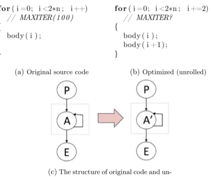
Compilers translate high level languages written by programmers into binary code fit for microprocessors. Modern compilers also typically apply hundreds of optimizations to deliver more performance. Some of them are local (i.e. at the granularity of the basic block), they usually do not challenge the consistency of flow information. Other optimizations radically modify the program control flow. As a result, it is usually very diﬃcult to match the structure of the binary code with the original source code, and hence to port flow information from high-level to low-level representations. Even when the structure of the binary and source code seem to match, there may be important changes of loop bound information, through optimizations such as loop unrolling or loop re-rolling. Figure 1 (shown in C language for readability, although it will be expressed in compiler Intermediate Representation (IR), or binary code) shows the application of loop unrolling. Loop unrolling in this example replicates the loop body twice in one iteration (body(i); ! body(i); body(i + 1);). The structure of the code does not change after the optimization. But the loop bounds are not the same (100 ! 50).

Using optimizing compilers is key to deliver performance. From the point of view of the programmer, compilers are black boxes that take source code as input, and produce binary code. Some compilers can produce dumps of the transformations they applied, but these dumps are very limited. Yet, modern compilers apply hundreds of transformations, some very aggressive, that radically modify the structure of loops

(20)

Introduction 9 for ( i =0; i <2∗n ; i++) // MAXITER(100) { body ( i ) ; }

(a)Original source code

for ( i =0; i <2∗n ; i +=2) // MAXITER? { body ( i ) ; body ( i +1); } (b)Optimized (unrolled)

(c)The structure of original code and

un-rolled code

Figure 1 –CFG matching and WCET overestimation

(consider unrolling, software pipelining, fusion, tiling, polyhedral transformations...) and functions (inlining, specialization, processing OpenMP directives).

Using the flow information obtained at the source code level, or using best-eﬀort methods for matching source code and binary code may be misleading. In the favorable case, the WCET is “simply” overestimated. Consider the example of Figure 1. The loop on the left has been annotated by the programmer. After optimization, in particular loop unrolling, the code will be similar to the right part of the figure. Both contain a single loop, and a tool could be tempted to match the CFGs and port the flow infor-mation to the binary representation. In this particular case, the result remains safe, but precision is lost since the new loop obviously iterates only 50 times at the maxi-mum, whereas the original loop iterates 100 times. On the other hand, loop rerolling (implemented in some compilers – including LLVM [LA04, LLVb] – to reduce code size) results in a increase of the number of loop iterations. Using graph matching for such loops would result in underestimated WCETs, that jeopardize the system safety.

So now we are facing the following issues:

• In order to derive better performance, modern compilers usually include opti-mizations. The quantity and type of the optimizations vary depending on the compilers.

• If the compiler optimizations are applied, the flow information may be modified. • When the flow information is modified, if we do nothing, better case is that the

(21)

10 Introduction

rerolling increases the number of loop iterations), or even cannot be got (e.g. loop unswitch and loop tiling add new loops whose loop bounds are unknown for WCET estimation).

• We have mentioned that graph matching may be unsafe as well.

• So a big problem comes: we cannot estimate a safe and as precise as possible WCET result with modern optimizing compilers.

The solution we proposed is to trace flow information in the optimizing compilers. Annotations are essential flow information to make WCET analysis more precise. So the traceability of annotations is the objective of our thesis.

The thesis is funded by the project W-SEPT1 _{which is a collaborative research}

project focusing on the precise estimation of the worst-case execution time and the identification and traceability of semantics information through the compilation flow from high-level language to C level and finally to binary level. The project is funded by ANR2 _{under grant ANR-12-INSE-0001, and supported by the competitiveness clusters}

Aerospace Valley3 _{and Minalogic}4_{. Our work is also partially funded by COST Action}

IC1202: Timing Analysis On Code-Level (TACLe)5_.

Contribution of the thesis

In this thesis, we propose a framework to systematically transform flow information from source code level down to binary code level. The framework defines a set of formulas to transform flow information for standard compiler optimizations. What is crucial is that transforming the flow information is done within the compiler, in parallel with transforming the code. There is no guessing what flow information have become, it is transformed along with the code they describe. In case the transformation is too complex to update the information, we may have the option to drop the information if the information is not necessary. In this way, we can guarantee that the result is safe, even though it will probably result in a loss of precision.

Our transformation framework is designed to transform flow information as ex-pressed by the most prevalent WCET calculation technique: Implicit Path Enumera-tion Technique (IPET) [LM95]. More precisely, flow constraints are expressed as linear relations between execution counts of basic blocks in the program control flow graph. As shown later in the thesis, the framework is general enough to cover all typical opti-mizations implemented in modern compilers.

The proposed framework was integrated into the LLVM compiler infrastructure. For the scope of this thesis, although formulas are more general, our experiments in LLVM will concentrate on loop bounds as sources of flow information.

1_{http://wsept.inria.fr}

2_{http://www.agence-nationale-recherche.fr}

3_{http://www.aerospace-valley.com}

4_{http://www.minalogic.org}

(22)

Introduction 11

Usually, programs spend most of the execution time in loops and in (recursive) func-tions. So determining loop bounds and function depths is an essential task for WCET estimation. Loop optimizations and function inlining in modern compilers make this task a challenge. Fortunately, in our implementation, loop bounds are traced carefully and all loop optimizations in LLVM are supported. Besides, inlining optimization is also included. Therefore, our framework and implementation accomplish this essen-tial and important task, and obtain the safe and tight WCET even with the compiler optimizations.

Our experimental results show that LLVM optimizations significantly reduce esti-mated WCETs.

Structure of the thesis

The contents of this thesis is organized as follows:

Chapter 1 gives an introduction to WCET, WCET estimation methods, WCET esti-mation tools and prototypes. Then, the most common WCET static analysis technique, IPET is described. At the end of this chapter, annotation languages are presented.

Chapter 2 describes the theoretical foundations required by our work. Then the main contribution of this thesis, a transformation framework, is proposed. Our transformation framework can trace flow information with compiler optimizations independently of the compiler framework. A summary of our supported compiler optimizations and their corresponding rule sets is presented in this chapter. At the end, we introduce and compare the research works related to our transformation framework.

An implementation of the proposed transformation framework within the LLVM compiler infrastructure is presented in Chapter 3. We present the overview of LLVM and then our traceability method and the corresponding modification of LLVM.

We provide experimental setup, results and their analysis in Chapter 4. Through the results and analysis, we can derive that:

• Flow information can be traced by our transformation framework during the com-piler optimizations.

• With our framework and implementation, we can estimate safe WCET. • Estimated WCET can benefit from compiler optimizations.

Finally, we conclude with a summary of the thesis contributions and plans for future work.

(23)

(24)

Chapter 1

WCET Estimation Techniques

This chapter gives an overview of Worst-Case Execution Time (WCET) estimation techniques and flow information transformation. After a generic introduction about WCET calculation techniques and tools in Section 1.1, the static WCET estimation method – Implicit Path Enumeration Technique (IPET) is described in Section 1.2. Afterwards, the diﬀerent existing annotations forms and the corresponding extraction methods are presented in Section 1.3.

1.1 Worst-Case Execution Time Analysis

“Deadlines” are the specified response time constraints which should be guaranteed by real-time systems. By the consequence of missing a deadline, real-time systems can be classified into the following three categories:

Hard Ensure that all deadlines are met. Missing a deadline is a total system failure. Firm Infrequent deadline misses are tolerable, but may aﬀect the quality of service.

The computation after its deadline is obsolete. Soft Deadline misses are tolerable, but not desired.

Hard real-time systems have to fulfill strict timing guarantees, otherwise catastrophic consequences may be caused. So to avoid this happening, the worst-case execution time (WCET) of the program needs to be known.

1.1.1 Worst-Case Execution Time and WCET estimation

WCET is an essential element for hard real-time systems. However computing the execution time of a program in the worst case is challenging. If the worst-case input for the program were known, we could derive a reliable guarantee based on the worst-case execution time. Unfortunately, in general this worst-case input is unknown and hard to derive.

(25)

14 WCET Estimation Techniques

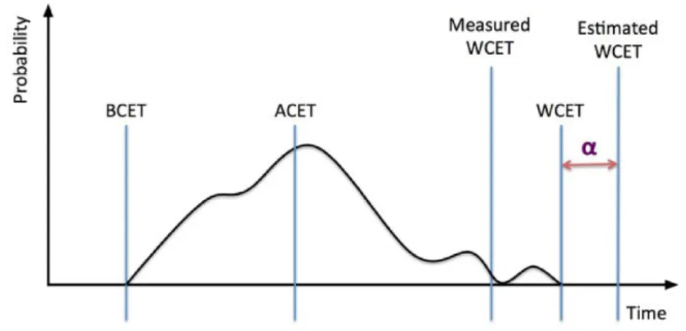
Figure 1.1 –Distribution of execution time and basic notions of timing analysis systems

The relevant typical terms used to describe the execution time of a program are depicted in Figure 1.1. The curve represents the probability of different execution times of a program with different input data and initial processor states. Usually, the curve applies to a given hardware/OS pair, and the execution times usually vary widely depending on the different program inputs. The best-case execution time (BCET) is the shortest execution time of the program. And worst-case execution time (WCET) is the longest execution time. Average-case execution time (ACET) lies between the BCET and WCET. ACET depends on the distribution of the execution time of a program. The average of the execution time observed for one input data set is called ACET. Average performance and worst-case performance are the most used.

Since worst-case performance is so important to hard real-time systems, how can we get WCET? WCET calculation techniques can be classified into two categories: static and measurement-based methods [WEE+_08].

Static methods abstract the program first, and then analyze the abstraction of the program and find all possible paths. Then the methods analyze the set of possible execution paths, and do not rely on execution of the program on real hardware or simulator which often needs complex equipment for the target system. They derive upper bounds of the WCET from the program structure and a model of the hardware architecture, and maybe together with some annotations. Annotations are the external information that are given explicitly by static analysis tools or program developers or users. More details about this category of methods are presented in [WEE+_08].

The estimated WCET in Figure 1.1 is derived by static methods. The estimated WCET is overestimated, because during the abstraction, the behavior of the processor cannot be predicted accurately, and a pessimistic result is usually used.

On the other hand, measurement-based methods use end-to-end measurements on the given processor or a cycle-accurate simulator, with a set of possible inputs data, in search for the input that exercises the longest execution path. The advantages for these methods are that they do not need to model hardware architecture and thus can be easy

(26)

Worst-Case Execution Time Analysis 15

to be applied to other new target systems. Besides, for complex programs and complex target systems, they are simpler to be applied. The measured WCET in Figure 1.1 is derived by these methods. In general, the WCET is underestimated, unless the worst case input is exercised by the measurements.

In Figure 1.1, ↵ is the diﬀerence between actual WCET and estimated WCET (↵ = estimated_W CET actual_W CET ). It can be used to explain the two main criteria of WCET estimation: safety and precision. Safety means that the estimated WCET must be higher than or equal to the actual WCET, i.e. ↵ should always be positive. This is essential for hard real-time programs to avoid severe damages. Precision means that the estimated WCET has to be as close as possible to the actual WCET. i.e. ↵ should be as small as possible. Actually, ↵ can be considered as explicit precision. A lack of precision may lead to a waste of hardware resources.

Static methods emphasize safety. These methods are based on the target hardware model that can capture the behavior of the processor. By design, static methods are guaranteed to identify the longest feasible execution path. And by using this longest feasible path it can produce the bound which can guarantee that the actual execution time will not exceed the bound, and therefore, are safe. However, the necessity for the specific model of hardware architecture and the possibly overestimated WCET esti-mate are the price paid for the safety. Nowadays, modeling hardware architecture and processor behavior is still a main technical problem.

The disadvantage of measurement-based methods is distinct: these methods may miss the actual worst case and may underestimate WCET, unless the target systems or test programs are simple enough, or all possible execution paths can be measured. So the underestimated WCET is impossible to be used in hard real-time systems. So we do not consider measurement-based techniques in this thesis.

Besides, there are some other timing analysis techniques, e.g. hybrid measurement-based analysis and probabilistic timing analysis.

Hybrid measurement-based analysis is similar to static methods. The diﬀerences are that hybrid timing analysis does not need to model hardware architecture, it derives execution times of small program segments by using measurement [KPW04, GBEL10, BMB10]. Then it combines them with static methods. The WCET estimated by this method is generally more accurate compared with static methods. However, there are kinds of drawbacks. For example, there is a possibility of underestimation; it adds an overhead which may disturb the accuracy and slow the program. The WCET analysis tool RapiTime [Rapb, Rapa] is an example.

Probabilistic WCET analysis [BCP02, BCP03] is a method combining static and measurement analysis in a probabilistic framework. The probability distribution of the WCET of a code fragment can be determined by this method. It extracts the program into a syntax tree in which the leafs are basic blocks and the inner nodes are the sequential, conditional and iterative parts. Then it uses a timing schema to represent the diﬀerent types of nodes in the syntax tree. A measurement approach can be used to record the actual execution time of each nodes. With these information, a WCET result can be derived.

(27)

1.1.2 WCET analysis tools and prototypes

In this subsection, we summarize the main WCET analysis tools and prototypes for the moment.

aiT aiT WCET Analyzer is the WCET analysis tool of AbsInt which is a software-development tools vendor based in Saarbrücken, Germany. The purpose of aiT [Abs, FH04, FHF07] is to obtain tight bounds for the WCET of tasks in real-time systems. It directly analyzes binary executables and statically analyzes a task’s intrinsic cache and pipeline behavior to compute correct and tight upper bounds for the WCET.

Bound-T The Bound-T timing analysis tool [Tid, HS02] provided by Tidorum Ltd computes an upper bound for the execution times fo programs by using static analysis of the machine code. Optionally, the tool can also get bounds on the stack usage of the subroutine, including called functions.

Chronos Chronos [oS, LLMR07] is an open-source static WCET analysis tool devel-oped at National University of Singapore (NUS). Chronos models various architectural features and their interactions for WCET analysis. By analyzing binary code, it con-structs control flow graph and extracts flow constraints. With these flow constraints, processor model, user configuration, additional flow information, Chronos determines an upper bound on the execution time of a program.

Heptane Hades Embedded Processor Timing ANalyzEr (Heptane) [CP00, IRI] is an open-source static WCET analysis tool designed by IRISA, Rennes (part of W-SEPT). Through statically analyzing source and/or binary code1_{, Heptane extracts control flow}

graph, loops, basic blocks and so on. With these information and loop annotations, it analyzes cache and computes the upper bounds on the execution time for many cache architectures.

OTAWA Open Tool for Adaptive WCET Analyses (OTAWA) [BCRS10, TRA] is a static WCET analysis tool developed by the TRACES team at IRIT labs, University of Toulouse, France (part of W-SEPT). OTAWA proposes abstract layers to make the analyses independently from the hardware and from the instruction set. By analyzing binary programs, the extracted flow information combining the information of the target hardware and annotations are used for the final WCET static analysis.

RapiTime RapiTime [Rapb, Rapa] is an automated measurement-based WCET anal-ysis tool developed by Rapita Systems Ltd. RapiTime measures the WCET result by running the real-time programs with a suite of tests. The users need to provide test

(28)

Static WCET Calculation Using IPET 17

suite to and can provide annotations in the code to guide the measurement. Benefit-ing from the measurement-based method, RapiTime does not rely on a model of the processor, and it can handle complex advanced architecture.

SymTA/P The purpose of SYMbolic Timing Analysis for Processes (SymTA/P) [oCNE] from IDA, TU Braunschweig is to obtain upper and lower execution time bounds of C programs by modeling and analyzing process behavior using execution cost inter-vals. The program structure and the execution context is considered in this tool.

SWEET SWEdish Execution Time tool (SWEET) [RtiV, Lis14] is a research proto-type provided by Mälardalen Real-Time Research Center (MRTC). It can translate dif-ferent code formats into their intermediate format ALF [GEL+_{09]. With ALF, SWEET}

analyzes and derives flow information automatically. At the end, it calculates safe bounds on the possible executions of a program.

T-CREST Time-predictable Multi-Core Architecture for Embedded Systems (T-CREST) [tcr, PPH+_{13] is a time-predictable system built collaboratively by}

indus-trial organisations and research and development organisations. It aims at the deriva-tion of the WCET of the hard real-time space applicaderiva-tions with multi-core technol-ogy. For this purpose, T-CREST proposes solutions on both the hardware (e.g. time-predictable caching) and the compiler infrastructure (e.g. LLVM compiler infrastructure and WCET aware optimizations). At the end, T-CREST provides a WCET analyzable multi-core system with high performance.

1.2 Static WCET Calculation Using IPET

The WCET calculation method used in the thesis is the most common technique, named IPET for Implicit Path Enumeration Technique [LM95, PS97]. This method operates on control flow graphs (CFG), extracted from binary code. IPET models the WCET calculation problem as an Integer Linear Programming (ILP) [GN72] formulation.

1.2.1 Integer Linear Programming (ILP)

At first, Linear Programming (LP) should be introduced. LP, also called linear opti-mization, is a method to process various linear inequalities relating to the requirements and find the best outcome of this mathematical model under these conditions. In a lin-ear program, there are variables, constraints, and an objective function. The variables stand for numerical values. Constraints are linear expressions and used to limit the values to a feasible region. The objective function should also be linear in the variables. Its declaration consists of one of the keywords minimize or maximize. It defines the quantity to be maximized or minimized subject to the constraints.

For ILP, it adds the requirements that some or all of the variables are restricted to be integers. ILP can be expressed in the following canonical form:

(29)

18 WCET Estimation Techniques Objective function M aximize X i2CF G fi⇥ Ti Structural constraints f1 =1 f_{1_2}+ f_{5_2}=f_{2_3}+ f_{2_4} = f2 f2_3=f3_5 = f3 f2_4=f4_5 = f4 f_{3_5}+ f_{4_5}=f_{5_2}+ f_{5_6} = f5 f_{5_6}=f6 Additional constraints f2  Xmax f2 Xmin f3 2 ⇥ f4

Figure 1.2 –CFG and WCET calculation using IPET

Variable xi 2 int (i = 1, 2, . . . , n)

Constraint Pn

i=1

aij⇥ xi bj (j = 1, 2, . . . , m)

xi 0 (i = 1, 2, . . . , n)

Objective function Maximize/Minimize Pn

i=1

ci⇥ xi

aij and bj are the parameters of the constraints, and ci are the parameters of the

objective function. All of them are integer constants.

1.2.2 Timing analysis with IPET

An example CFG is depicted in the left part of Figure 1.2. The example program includes one loop, depicted by a rectangular box. Notations Xmin and Xmax state

that the loop iterates at least Xmin times, and at most Xmax times. They are used in

additional constraints. (More information in Section 2.1.2)

The right part of Figure 1.2 depicts the ILP system used to calculate the WCET. Every basic block i has a worst-case execution time, denoted as Ti, and considered

constant in the ILP system. Calculating the WCET is done by maximizing the objective function, in which fi is variable and represents the execution count of basic block i.

(30)

Flow Information and Annotation 19

structure of the CFG and are generated automatically. From top to bottom, the first one states that the entry point to be analyzed is executed exactly once. The next constraints state that the execution count of a basic block is equal to the sum of the execution counts of its incoming edges, as well as outgoing edges, where fi_j represents

the execution count of the edge from node i to j.

Finally, additional constraints specify flow information that cannot be obtained directly from the control flow graph. The first kind of additional information is loop information (f2  Xmax and f2 Xmin in the example). It gives the maximum

number of iterations for loops, and is mandatory for WCET estimation. Some other linear constraints such as f3  2 ⇥ f4 may also be specified to constrain the relative

numbers of executions of basic blocks in the CFG. Additional constraints come from the semantics of the programs and cannot be derived easily, so they may be inserted manually by the programmer, through annotations, or be obtained automatically using static analysis tools.

1.3 Flow Information and Annotation

Previous section mentioned that static analysis methods may need some annotations (e.g., loop bounds, infeasible paths and so on) to derive upper bounds for the execu-tion times of programs on a given platform. In fact, WCET estimaexecu-tion usually needs manual annotations or assertions to define essential information. Information on the flow of control of applications improves the tightness of WCET estimates. Beyond loop bounds, which are mandatory for WCET calculation, examples of flow informa-tion include infeasible paths, contextual informainforma-tion, or other properties constraining the relative execution counts of program points. An annotation language is used to annotate the flow information and make the information available to the subsequent WCET analysis. The following seven pivotal points decide the design of an annotation language and have an impact on its usability. They are related to both the WCET analysis tools and the target programs.

• The need for annotations • The form of annotations • The content of annotations • The supported language • The placement of annotations • The level of annotation

(31)

1.3.1 The need for annotations

The WCET analysis methods and tools vary widely. But many of them need annotations for precise WCET estimation. Sometimes, the annotations improve even the eﬃciency of the estimation.

1.3.2 The form of annotations

Normally, the form of annotations is special to its own WCET analysis tool. It relates to the placement, the level, even the method of addition. For example, for external separate annotations, Extensible Markup Language (XML) [BPSM+_{98], as a simple}

and universal format, is used widely to represent annotations.

One example is an XML-based representation [PM14] proposed by Parsa et al. They use this XML-based annotation to store the information from the analysis of program and to provide to other WCET analysis tools for precise WCET estimation.

FFX [BCdM+_{12] is another XML-based annotation format. Benefiting from the}

XML standard, it is easy to create, understand and use among diﬀerent WCET tools.

1.3.3 The content of annotations

Theoretically and ideally, the annotations should contain all flow information (loop information, infeasible paths, contextual information and so on). However, considering the limitation of annotation format, the need of WCET analysis tools, and diﬃculty of flow information acquisition, annotations should choose the appropriate content. But for almost every annotation, loop bound is the essential part.

1.3.4 The supported language

Most annotations support a single programming language (based on WCET analysis tools, and for now C language is supported most widely). There are a few annotations that can support multiple languages.

1.3.5 The placement of annotations

There are two primary ways to keep annotations: inside the source code or in a separate file. None of them is consistently superior to the other. Normally, the annotations are usually added inside the source code when the annotations must be added manually. Because in this way, it is much easier and less error-prone. On the contrary, when the annotations are derived by the static analysis tools, writing into a separate file is more convenient for both the analysis tools and WCET estimation tools.

1.3.6 The level of annotations

Annotations can be added at high-level source code or low-level machine code.

The advantage of addition at machine code level is the convenience of usage. Because the WCET estimation is also at machine code level, the annotations can be used directly.

(32)

Flow Information and Annotation 21

The addition of annotations at this level is usually through two methods. One is to read and analyze machine code. This is diﬃcult for the programmers, users and the analysis tools. Another is to map with source code. This is typically non-trivial. When the optimizations are applied, this becomes diﬃcult and error prone. One method to maintain the mapping between source code and machine code is to define a set of language constructs: anchors [KKP+_{07]. which can be recognized after compilation.}

Compared with machine code level, adding annotations at source code level is easier for both programmers and analysis tools. And these annotations are easier to under-stand and verify. So, normally, source code level annotations are chosen in most cases.

1.3.7 The method of annotations addition

Annotations can be obtained via two basic methods: static analysis or annotations added by the application developers or users.

Manual annotations are an easy and convenient way to assist non-perfect analyses. Usually, they are added by the users who know the code well, e.g. the program develop-ers. However, manual annotations are potentially error-prone and may yield incorrect WCET estimates.

In order to get the annotations automatically, the static analysis tools are required. With the development of the techniques of flow information extraction, more and more annotation languages use the automatic additional methods.

At the same time, more and more methods of flow information extraction are pro-posed. Here are several examples:

Gustafsson et al. [GESL06] propose a method called abstract execution. This method can automatically calculate loop bounds and infeasible paths. Their method can calculate nested loop bounds. They verify their method by using Mälardalen bench-mark suite.

Blackham et al. [BLH14] propose an infeasible paths detection method called Trickle. This method analyzes the binary programs and detects infeasible paths within the CFG to refine WCET estimations.

Holsti et al. [HGKL14] use the program-representation language ALF to combine two analysis tools: Bound-T and SWEET. The combination can resolve the analysis of dynamic branches at binary code level. They can generate an annotation file containing the analyzed control flow information. This annotation file is used to guide the further WCET estimation.

Bonenfant et al. [BdMS08, dMBBC10] develop a static loop bound analysis tool called oRange. The tool is based on flow analysis and abstract interpretation, and can extract and provide loop bound values or equations, non-recursive function calls and other flow information. The provided flow information can be used in static WCET analysis.

There are still many automatic methods concentrating diﬀerent kinds of flow in-formation: branch constraints detection and exploitation [HW02], loop bounds extrac-tion [LCFM09] and so on.

(33)

Nowadays, the hybrid methods are used by some WCET tools. They base on au-tomatic extraction, and use manual addition to fix the unobtainable part, e.g. aiS and Bound-T annotation language (introduced in the next subsection).

1.3.8 Summary of annotation languages

Here, we give a summary of WCET annotation languages. More detailed WCET an-notation languages description and systematic comparison are presented in [KKP+_07,

KKP+_{08, KKP}+_11].

Real-Time Euclid [KS86] is one of the first language designed specifically to feature annotations for timing analysis in real-time systems. Only the specification of loop bounds in for loops are supported.

Another early annotation is proposed by Park et al. in [PS90, Par93, Cha94]. They define the information description language (IDL) as an interface language for users to provide and express flow information. This approach uses IDL to perform the mapping from the object code to the source code. Path patterns of explicit execution order can be expressed by this annotation, and this is also its advantage.

WCETC [Kir02] is designed as a new programming language. It is based on ANSI C

and extends it with new grammar. Benefiting from the new grammar, additional flow information including loop bounds or infeasible/feasible paths can be specified directly in the source code. With the additional flow information is used to estimate the WCET. The advantage of this annotation is that it can annotate flow information exactly at the location where the program should be described.

The annotation language of Heptane [IRI] is designed to provide loop bounds. Its diﬀerence is that these annotations can be provided in two ways: add loop bounds inside each loop in the C source code; provide an external XML-based annotation file in which the loop bounds are given and the order of loops should be the same as in the compiled binary code.

Mok et al. [Che87, MACT89] propose the Timing Analysis Language (TAL). TAL is an integral part of the timing analysis system. It consists of multiple tools. The annotation tool can analyze C source code and automatically generate the annotations of the C code with default assumptions about the program’s behavior. Then a mod-ified C compiler translates annotated C programs to annotated assembly programs, because timetool which calculates the execution time works only on assembly code. The advantage of this annotation is that it may contain arbitrary calculations.

The Bound-T applies a data-flow analysis to automatically compute loop bounds. When the loop bounds could not automatically be bounded, it involves user-assistance. These automatic and manual information are stored in a separate file. Then all these information are used for the WCET estimation.

aiS is the annotation language of aiT. aiT applies an analysis to automatically calculate flow information. It also needs additional annotations provided by users in the aiS format called AIS file. The AIS file needs to provide not only loop bounds, but also recursion bounds, even the targets of calls and branches.

(34)

Summary 23

Both of these two annotation language are the language of commercial WCET anal-ysis tools, and they use hybrid WCET annotation addition method.

1.4 Summary

This chapter describes the notion of WCET and WCET analysis methods, then lists the WCET analysis tools and prototypes. Then we introduces the most common WCET static analysis technique: IPET. At the end of this chapter, another important notion in this thesis is presented: annotations. Through this chapter, we know that WCET is essential for hard real-time systems. However, the optimizations in modern compilers make the WCET estimation complex. Because, the optimizations break the link be-tween the annotations and the code, the annotations cannot be used directly. Our thesis focuses on this issue, and fortunately, we propose a solution: transformation framework of flow information. In the next chapter, we will present our transformation framework.

(35)

(36)

Chapter 2

Transformation Framework

In this chapter, the theoretical foundations required by our transformation framework are introduced firstly in Section 2.1. We need flow information to calculate the WCET bound. The flow information is translated into linear constraints (shown in Section 2.2). However, some optimizations may have an eﬀect on these constraints, furthermore aﬀect the calculation of WCET. So in order to get more precise estimated WCET bound after the optimizations, we need a method which can declare the flow information transfor-mation and update the constraints.

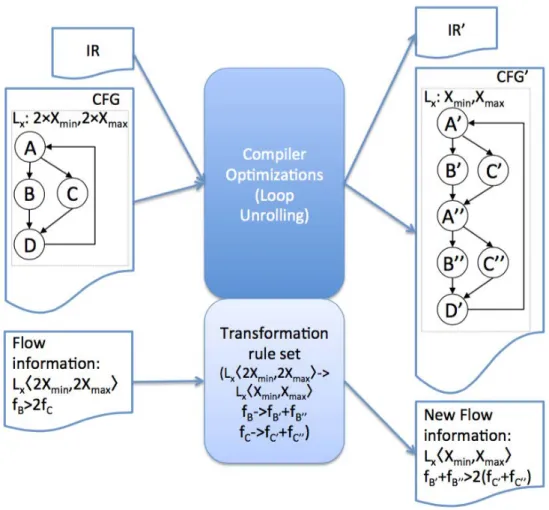
So in Section 2.3, the main contribution of the thesis is introduced. we propose a transformation framework that conveys flow information from source code level to machine code level with the compiler optimizations. The transformations are expressed in an abstract way, independently of the compiler infrastructure in which they will be integrated. In this part, we introduce the transformation framework with the following aspects: transformation rules, the manipulation and its influence on WCET estimation. Afterwards, an overview of the transformation framework is provided in Section 2.4.

Then in Section 2.5, the code optimizations performed by the compiler and the advantages of these optimizations are described according to their impact on the con-trol flow and WCET analysis. For each compiler optimization, our transformation framework, defines a set of formulas, that rewrite available flow constraints into new constraints according to the code transformation. Then these new constraints can be used for the WCET estimation.

At the end, in Section 2.6, the related work to the traceability of flow information and WCET estimation with compiler optimizations are described.

2.1 Flow Information

Flow information is the information of the control flow of a program. Flow informa-tion can be expressed explicitly by the control flow graph (CFG), also by addiinforma-tional information provided externally.

Through analyzing the CFG, we can get structurally feasible paths. When the compiler optimizations are applied, the CFG is usually modified. These flow information

(37)

26 Transformation Framework

for ( int i =0; i<n ; i++) { i f ( a [ i ] >0) b [ i ]=b [ i ]+ i ; else b [ i ]=a [ i ]+n ; }

Figure 2.1 –Example of control flow graph (CFG)

can be updated automatically according to the new CFG. Unfortunately, the relation between the external information and the CFG of the source code is broken by the optimizations.

The rest of this section explains the notions and definitions about flow information.

2.1.1 The program representation

Our transformation of flow information operates on the program control flow graph (CFG) [All70]. For presentation clarity, we will concentrate in this thesis on a single CFG, although our transformation framework supports multiple functions and function calls. The CFG is important, because it is used in most compilers, and is essential to many compiler optimizations and static analysis tools.

At first, the definition of basic block is given because it is used in the definition of CFG.

Definition 1 A basic block is a straight-line piece of the code within a program with only one entry point and only one exit point, i.e. without any jumps except the last instruction or jump targets except the first instruction.

Here, the code can be assembly code, intermediate representation or some other sequence of instructions.

Definition 2 A CFG is a representation using graph notation. A CFG is a (possibly cyclic) directed graph made of a set of nodes N representing basic blocks, and a set of edges E representing possible control flows between basic blocks.

In the example program of Figure 2.11_{, we have:}

(38)

Flow Information 27 CFG = {N , E} N =_{B1, B2, B3, B3, B4, B5, B6} E = {B1 ! B2, B2 ! B3, B2! B4, B3 ! B5, B4 ! B5, B5! B2, B5 ! B6} 2.1.2 Loop description

During the flow information, loop bound is the most important notion. Because loop bound information is the necessary information to derive WCET estimate.

Firstly, we need to define strongly connected component which is the most general looping structure.

Definition 3 A strongly connected component of a flow graph G = (N, E) is a subgraph Gs = (Ns, Es), in which there is a path that includes only edges in Es from

every node in Ns to every other node in Ns.

Definition 4 A loop is a strongly connected component of the CFG.

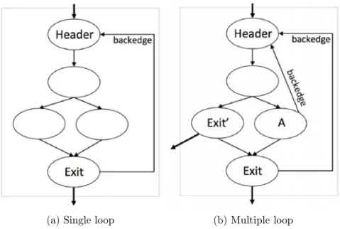
(a) Single loop (b) Multiple loop

Figure 2.2 –Loops

Then, we introduce the following properties of loops:

Entry nodes/Loop headers are the nodes into the loop from outside. They domi-nate all nodes in the loop2_{. In this thesis, we only consider the loops with unique}

loop header (as shown in Figure 2.2).

(39)

Exit nodes are nodes with edges going to the nodes outside of the loop. There can be several exit nodes, e.g. in the example of Figure 2.2b, there are two exit nodes: the exit node similar to the one of the single exit node loop and the exit node Exit0 _{which can be brought by instruction break.}

A backedge is a part of the loop. It is an edge from node A to node B if B dominates A (A, B 2loop). A loop can have more than one backedge. For example, in the example of Figure 2.2b, besides the backedge similar to the one of the single backedge loop in Figure 2.2a, edge A ! Header is another backedge which can be created by instruction continue. Optimization Loop Simplify3 _{can turn the loop}

into single backedge loop. For single backedge loop, backedges can be used to represent the iteration count of the loop.

Figure 2.2 shows two typical loop examples. The left one is a typical loop with single entry node and single exit node. The right one is a loop with multiple exit nodes and multiple backedges. In fact, a loop can have multiple entry nodes, exit nodes or multiple backedges, while in this thesis, we consider only reducible loops: single entry node, one or multiple backedge and one or multiple exit nodes.

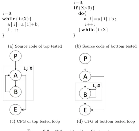
i =0;

while ( i<X){ a [ i ]=a [ i ]+b ; i ++;

}

(a)Source code of top tested

i =0; i f (X>0){ do{ a [ i ]=a [ i ]+b ; i ++; }while{ i <X} }

(b)Source code of bottom tested

(c)CFG of top tested loop (d)CFG of bottom tested loop

Figure 2.3 –Diﬀerent location of test nodes.

3_{Loop simplify optimization transforms natural loops into simpler ones. For example, it guarantees}

the loop with a single edge from outside of the loop to the loop header; with a single backedge and so on. In this way, further optimizations are simpler and more eﬀective to apply.

(40)

Flow Information 29

Figure 2.3c and Figure 2.3d show two diﬀerent CFG of loops. Actually, these two loops do the same function (refer to the source code Figure 2.3a and Figure 2.3b). Node B in both loops is executed X times. But for node A in Figure 2.3c, it is executed X + 1 times. The loop bounds of both loops are X. So for the bottom tested loop, the execution count of each node in the loop body equals to loop bounds. The test node in top tested loop is executed one more time than loop bound. So for uniformity, we define loop bounds as:

Loop bounds are the maximum number of executions of the nodes in the loop body except the node(s) testing the loop exit4_.

A Local loop bound represents the maximum number of iterations of a loop for each entry.

A Global loop bound is an upper bound on the execution count of a loop in a whole program. It is considered in nested loops.

for ( i =0; i <10; i++)

a [ i ]=a [ i ]+1; for ( i =0; i<n ; i++)a [ i ]=a [ i ]+1;

(a) Loop A (b) Loop B

Figure 2.4 –Example of Loop Bounds

Sometimes, the loop bounds are not fixed, they can be intervals. For example, in Figure 2.4, the loop A has a fixed loop bound 10. For loop B, its loop bound depends on the value of n. When 10  n  20, the loop bounds of loop B range from 10 to 20. We call the endpoints of the loop bound interval (a, b for interval [a,b]) the lower loop bound (for a) and the upper loop bound (for b). So for loop B, its lower loop bound is 10 and upper loop bound is 20. In this thesis, the lower loop bound is expressed as LBmin and the upper loop bound LBmax.

When we mention global loop bound, we refer to nested loop. Now we give the definition of this notion.

Definition 5 Nested Loopsare a set of loops in which each loop except the outermost one is within the body of another.

Definition 6 Perfect loop nest5 _{means that except the innermost loop, each loop}

contains only another loop in the nest.

The proposed framework for traceability of flow information in the next chapter assumes reducible nested loops. Information on loop nesting is captured through the Loop Scope data structure.

4_{If the test node is the only node in the loop, the loop bound is its maximum execution number.}

(41)

Definition 7 Loop Scopesare the code boundaries of loops.

The information is made of a set of pairs hLo, Lii with Lo and Li as loops. Li is the

inner loop and is completely nested in the outer loop Lo. This data structure is useful

because some compiler optimizations involve multiple loops (e.g. loop interchange), their maximum number of iterations have to be modified jointly.

Figure 2.5 –Running example with nested loops

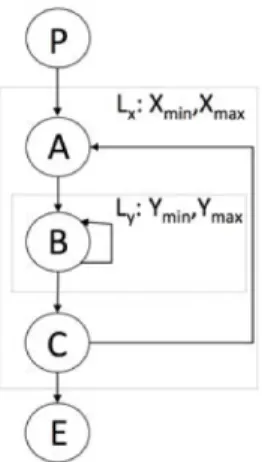
The Loop Scope data structure for our running example depicted in Figure 2.5 contains:

LoopScope = {h_, Lxi , hLx, Lyi}

with “_” denoting the absence of enclosing loop for the outermost loop.

for ( i =0; i <10; i++) for ( j =0; j <10; j++) a [ j , i ]=a [ j , i ]+1; for ( i =0; i <10; i++) for ( j =0; j<i ; j++) a [ j , i ]=a [ j , i ]+1;

(a) Loop Nest A (b) Loop Nest B

Figure 2.6 –Local/Global Loop Bound

When the loop is nested, the local bounds of all the loop bounds involved in the nest are estimated separately as if there was no nesting, but the global loop bounds of the innermost loop need a summation of the maximum iteration number in each iteration of the outer loop. Using local loop bound and global loop bound has no diﬀerence except several special cases e.g. triangular loops. For example, considering the loop nest A in Figure 2.6, the local loop bounds of the outermost and innermost loop are both 10, and the global loop bound of the innermost loop body a[j, i] = a[j, i] + 1 is 100 which is equal to the product of local outermost loop bound and local innermost loop bound. However, for the loop nest B, the situation is diﬀerent. The local loop bound is the same as nested loop A. The global execution count of the innermost loop body is 45, not 100.

(42)

Flow Information 31 i f ( x>5){ y=2; a=3; z=a+y ; } else y= 2; i f ( x>0) z++; else { z ; b=4; }

Figure 2.7 –Example of infeasible paths

Knowledge of global loop bounds can tighten WCET estimates. However, the obten-tion of global loop bound is a challenge, and most WCET analysis tools do not support it. Our transformation framework and our implementation support local loop bound. And in the rest of the thesis, when we mention loop bounds, it should be considered as local loop bound by default.

2.1.3 Infeasible paths

Definition 8 Infeasible Paths [Kou96, APT00, GEL06] are the paths which are executable according to the CFG, but not feasible when considering the semantics of the program, the context and possible inputs.

Dependencies are the primary reason for infeasible paths. The classical example of an infeasible path is two consecutive if-then-else structures with interdependent conditions. The example in Figure 2.7 illustrates a very simple example with an infeasible path. The true branch B of the first conditional statement and the false branch F of the second conditional statement are in conflict. Because when the true branch B is taken, i.e. x is larger than 5 and also larger than 0, the false branch F is never taken in this situation. So the path A B D F is never taken and it is an infeasible path.

Another case is that when the variable x is an input, and if its input value is 2, the path A B is infeasible. This kind of infeasible path belongs to input-sensitive infeasible paths.

Information on infeasible paths is not a mandatory information for WCET estima-tion, just can make WCET estimates tighter. For example, in Figure 2.7, without the information of infeasible paths, the WCET analysis tools should use A B D F to