HAL Id: hal-03095143
https://hal.archives-ouvertes.fr/hal-03095143
Submitted on 20 Jan 2021
HAL is a multi-disciplinary open access
archive for the deposit and dissemination of
sci-entific research documents, whether they are
pub-lished or not. The documents may come from
teaching and research institutions in France or
abroad, or from public or private research centers.
L’archive ouverte pluridisciplinaire HAL, est
destinée au dépôt et à la diffusion de documents
scientifiques de niveau recherche, publiés ou non,
émanant des établissements d’enseignement et de
recherche français ou étrangers, des laboratoires
publics ou privés.
A climate model inter-comparison of last interglacial
peak warmth
Emma Stone, P Bakker, S Charbit, S Ritz, V Varma
To cite this version:
Emma Stone, P Bakker, S Charbit, S Ritz, V Varma. A climate model inter-comparison of last
interglacial peak warmth. Past Global Changes Magazine, Past Global Changes (PAGES) project,
2013, 21 (1), pp.32-33. �hal-03095143�
32
PAGES news • Vol 21 • No 1 • March 2013
Scienc
e H
ighligh
ts: I
nv
estiga
ting P
ast I
nt
er
glacials
A climate model inter-comparison of last interglacial
peak warmth
Emma J. StonE1, P. BakkEr2, S. CharBit3, S.P. ritz4and V. Varma5
1School of Geographical Sciences, University of Bristol, UK; [email protected]
2Earth & Climate Cluster, Department of Earth Sciences, Vrije Universiteit Amsterdam, The Netherlands; 3Laboratoire des Sciences du Climat et
de l'Environnement, CEA Saclay, Gif-sur-Yvette, France; 4Climate and Environmental Physics, Physics Institute and Oeschger Centre for Climate
Change Research, University of Bern, Switzerland; 5Center for Marine Environmental Sciences and Faculty of Geosciences, University of Bremen,
Germany
A last interglacial transient climate model inter-comparison indicates regional and inter-model differences in
timing and magnitude of peak warmth. This study reveals the importance of different climate feedbacks and
the need for accurate paleodata in terms of age, magnitude and seasonality to constrain model temperatures.
P
aleorecords and climate modeling studies indicate that Arctic summers were warmer during the last interglacial (LIG, ca. 130 to 115 ka BP) and global sea level was at least 6 m higher than today (Dutton and Lambeck 2012; Kopp et al. 2009), implying a reduction in the size of the Greenland and Antarctic ice sheets (Siddall et al. this issue). Previous snapshot climate model simulations for the LIG have shown summer Arctic warming of up to 5°C compared with the present day (Kaspar et al. 2005; Montoya et al. 2000), with the largest warming in Eurasia and the Greenland region. The LIG period provides an opportunity to test the current suite of climate models of varying degrees of complexity, under forcings that re-sult in a warmer than present climate. To date, however, there has been no standardized inter-comparison of LIG climate model simula-tions.Five European modeling groups (form-ing part of the Past4Future project) have per-formed experiments in order to characterize the response of the climate system to LIG changes in various climate forcings and bio-physical feedback processes. These forcings and feedbacks include greenhouse gas con-centrations (GHG), orbital configuration (ORB), vegetation feedbacks (VEG), and changes in ice sheet geometry (ICE). A key aim of this inter-comparison is to perform a number of sensitivity studies (e.g. ORB only, ORB+GHG, ORB+GHG+VEG, ORB+GHG+ICE) to ascertain the relative importance of the forcings and feedbacks in determining the trends and vari-ability of LIG climate.
The Past4Future project has enabled the first long (> 10 ka) transient standard-ized inter-comparison for the LIG to be real-ized. These simulations consist of a range of model complexity with various forcings and feedbacks included: one full general circula-tion model CCSM3 (ORB; Collins et al. 2006; Yeager et al. 2006), one low-resolution gen-eral circulation model, FAMOUS (ORB+GHG; Smith 2012; Smith et al. 2008), and three Earth System Models of Intermediate Complexity: 1) CLIMBER-2 (ORB+GHG; Petoukhov et al. 2000), 2) Bern3D (ORB+GHG+ICE; Müller et al. 2006;
Ritz et al. 2011), and 3) LOVECLIM (ORB+GHG; Goosse et al. 2010). CLIMBER-2, Bern3D, FAMOUS, and LOVECLIM use GHG and orbital forcings that conform closely to a set of stan-dards described by the Paleo-modeling Inter-comparison Project (PMIP3) while CCSM3 uses the same orbital configuration but with green-house gas values fixed according to mean LIG values. Bern3D is the only model that pre-scribes ice-sheet changes (and an associated freshwater forcing) by including the effect of remnant Northern Hemisphere ice sheets from the penultimate glaciation (all other models use present day ice sheet geometry).
One of the difficulties in understanding the response of the climate to LIG forcings is the lack of consensus in the paleodata on the timing of peak interglacial warmth in dif-ferent regions of the Earth (e.g. The Nordic Seas and North Atlantic; Govin et al. 2012; Van Nieuwenhove et al. 2011). The interpretation of temperature signals of different resolution
and seasonality obtained from paleoclimatic archives is also contentious (Jones and Mann 2004). Our climate modeling approach aims to inform on the spatial and temporal differences in peak warmth observed in the data, as well as on assessing the robustness of our climate model results (Bakker et al. 2013). Through this task it is also possible to gain an understanding of the climate feedbacks (e.g. changes in ocean overturning circulation and sea-ice) that are at play resulting from changed GHG concentra-tions and astronomical forcing.
How does LIG summer temperature
response compare in four different
regions of the Earth?
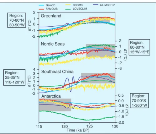
Figure 1 shows the 50-year summer average surface air temperature anomalies over four defined regions of the globe where paleodata exist for the time period 130 to 115 ka BP. These model results demonstrate not only the differ-ences in the timing of peak summer warmth
Figure 1: Summer 50-year global mean temperature anomalies spanning the LIG (ca. 130 to 115 ka BP) for five climate models of varying complexity. Note that these anomalies are calculated with respect to a preindustrial equilibrium climate representative of 1850 AD. For more details with respect to model setups and forcings see Bakker et al. (2012). The range in timing of the peak interglacial warmth is indicated by the gray bars.
33
PAGES news • Vol 21 • No 1 • March 2013
Scienc
e H
ighligh
ts: I
nv
estiga
ting P
ast I
nt
er
glacials
between regions but also discrepancies be-tween the models themselves. Greenland shows peak summer warmth during the early LIG for all five models with positive tempera-ture anomalies compared with pre-industrial values ranging from ~0.1 to 1°C, albeit sub-stantially smaller than the +5°C anomaly ob-tained from ice core records (e.g. NorthGRIP Project members 2004). Future simulations, which include a reduced Greenland ice sheet, may reconcile this difference between models and data.
Simulated maximum summer tempera-ture anomalies for the Nordic Seas (-1.0 to 1.0°C) and southeast China (~0 to 3°C), how-ever, indicate a less robust result between the models in terms of timing and temperature change. We compare our model results with a recent data synthesis by Turney and Jones (2010) and show that no model produces a maximum summer temperature anomaly as large as that inferred from paleodata (up to +9°C) for the Nordic Seas. This discrepancy could be due to missing feedback processes in the model simulations (such as vegetation changes), misrepresentation of ocean circula-tion and a simplistic representacircula-tion of sea ice dynamics. Furthermore, the discrepancy could be larger still because the Turney and Jones (2010) data synthesis has been interpreted as an annual rather than a summer temperature signal. We also note that the Bern3D model simulation, which includes remnant ice sheets from the previous glacial, shows a delay in peak LIG warmth for Greenland and the Nordic Seas compared with the other models indicat-ing the importance of this feedback.
In contrast to Greenland, timing of sum-mer peak warmth in the Southern Hemisphere shows a substantial delay, with peak summer values (from -1 to 0.1°C) only being obtained after 120 ka BP. This contradicts a recent pa-leodata study (Govin et al. 2012) suggesting Southern Hemisphere peak warmth actually preceded Northern Hemisphere warming dur-ing the early part of the LIG.
Seasonal timing of LIG maximum
warmth
Figure 2 shows the spatial distribution of tim-ing of maximum LIG warmth durtim-ing January and July. Superimposed are the four regions described above and given in Figure 1. During Northern Hemisphere winter (January), there is large variability between models in the tim-ing of maximum warmth rangtim-ing from ca. 119 to 128 ka BP over Greenland and the Nordic Seas. We relate these discrepancies at high northern latitudes during winter to differences in sea-ice feedback mechanisms (Bakker et al. 2013). In contrast, Southern Hemisphere win-ter (July) temperatures over Antarctica show less variability in timing of peak winter warmth. The temperature anomalies reach a maximum
ca. 128 ka BP for CLIMBER-2, LOVECLIM and FAMOUS relating to those simulations which include the same forcings. There is a delay in peak warmth for Bern3D and CCSM3 (CCSM3 does not include transient GHGs and Bern3D includes remnant ice sheets and changes in freshwater forcing).
During the northern summer months, the inter-model comparison shows consistent timing of maximum warmth at high latitudes, ranging between ca. 124 and 128 ka BP (Fig. 2). This consistency is also the case for the Southern Hemisphere in July, but austral sum-mer maximum warmth occurs much later (af-ter 118 ka BP). In northern mid-to-low latitude regions, such as southeast China, all model simulations show reasonably similar results in timing of maximum warmth during the northern summer (July) and winter (January) months.
Perspectives
The Past4Future LIG modeling group provides important information for the data commu-nity regarding locations for relevant potential new paleoclimatic data. We also provide in-sights into understanding the mechanisms that result in differences in peak warmth tim-ing and magnitude from proxy data tempera-tures around the world. Our results inform on the impact of remnant ice sheets and the importance of understanding the sensitivity of
climate feedbacks during periods of enhanced warming. Part of the Past4Future data and modeling community remit is to reconstruct a coherent picture of LIG climate with the use of climate models to explain the temperature patterns observed in proxy observations. The next stage will be to take part in a detailed multi-millennial scale temperature compari-son between model and data for the LIG. This will aim at understanding and explaining the differences between climate model results and how they might constrain future predic-tions of global warming.
Selected references
Full reference list online under:
http://www.pages-igbp.org/products/newsletters/ref2013_1.pdf Bakker P et al. (2013) Climate of the Past 9: 605-619 Govin A et al. (2012) Climate of the Past 8: 483-507 NorthGRIP Project members (2004) Nature 431: 147-151 Turney CSM, Jones RT (2010) Journal of Quaternary Science 25: 839-843 Van Nieuwenhove N et al. (2011) Quaternary Science Reviews 30:
934-946
Figure 2: Timing of maximum LIG warmth for the months January and July for the five climate models of varying complexity. The regions defined in Figure 1 for Greenland, Nordic Seas, southeast China, and Antarctica are depicted by the white boxes . Figure modified from Bakker et al. (2013).