A regularized approach of instances x variables co-clustering for exploratory data analysis

(1)

THÈSE DE DOCTORAT

Université Paris 1 panthéon-Sorbonne

École doctorale : Sciences Mathématiques de Paris Centre (ED 386)

présentée par

Aichetou Bouchareb

Pour obtenir le grade de

Docteur

de l’

Université Paris 1 panthéon-Sorbonne

Spécialité Mathématiques Appliquées

A regularized approach of instances

_×

variables co-clustering for exploratory

data analysis

Soutenue le 28 Novembre 2018 devant le jury composé de :

M. Julien Jacques PR Université de Lyon - Lyon 2 (Rapporteur)

M. Mohamed Nadif PR Université Paris Descartes (Rapporteur)

M. Gilbert Saporta PR émérite Conservatoire National des Arts et Métiers (Examinateur)

M. Gilles Bisson CR CNRS Laboratoire d’Informatique de Grenoble (Examinateur)

M. Fabrice Clérot Chercheur senior Orange Labs (Examinateur)

M. Fabrice Rossi PR Université Paris 1 Panthéon-Sorbonne (Directeur)

(2)

(3)

Abstract

Co-clustering is a class of unsupervised data analysis techniques aiming at ex-tracting the underlying dependency structure between the rows and columns of a data table in the form of homogeneous blocks, known as co-clusters. These techniques can be distinguished into those that aim at simultaneously clustering the instances and variables, and those that aim at clustering the values of two or more variables of a data set. Most of these techniques are limited to variables of the same type, and are hardly scalable to large data sets while providing easily interpretable clusters and co-clusters.

Among the existing value based co-clustering approaches, MODL is suit-able for processing large data sets with several numerical or categorical vari-ables. In this thesis, we propose a value based approach, inspired by MODL, to perform a simultaneous clustering of the instances and variables of a data set with potentially mixed-type variables.

The proposed co-clustering model provides a Maximum A Posteriori based summary of the data that can be used as it is for exploratory analysis of the data. When the summary is large, exploratory analysis tools, such as model coarsening, can be used to simplify the co-clustering which facilitates the interpretation of the results. We show that the proposed co-clustering approach can handle large data and extract easily interpretable clusters from mixed data with more than 10 millions observations. We also show the ro-bustness of the approach, its capacity to extract inter-dependence between the variables, and its good behavior in extreme cases such as in the case of pattern-less data and in the case of perfectly correlated variables.

(4)

(5)

Résumé

Le co-clustering est une classe de techniques d’analyse non supervisée visant à extraire la structure sous-jacente de dépendance entre les lignes et les colonnes d’un tableau de données sous la forme de blocs homogènes, appelés co-clusters. Ces techniques peuvent être différenciées en deux types: celles qui effectuent un groupement simultané des instances et des variables d’une matrice de données, et celles qui effectuent un groupement des valeurs de deux ou plusieurs variables. Toutefois, la plupart de ces méthodes se lim-itent à des variables du même type et sont difficilement adaptables à des bases de données de grande taille, tout en fournissant des clusters facilement interprétables.

Parmi les méthodes basées sur la classification des valeurs, MODL per-met de traiter des données de grande taille et de réaliser une partition de plusieurs variables, numériques et/ou catégorielles. Dans cette thèse, nous proposons une approche de classification croisée, inspirée de MODL et basée sur le groupement des valeurs, pour effectuer un groupement simultané des instances et des variables d’un ensemble de données contenant des variables potentiellement de type mixte.

Le modèle proposé est basé sur l’estimation par Maximum A Posteri-ori et fournit un résumé de la base de données, exploitable pour l’analyse exploratoire. Lorsque ce résumé est très grand, des outils d’analyse ex-ploratoire, comme la fusion successive des clusters, peuvent être utilisés pour simplifier le co-clustering, ce qui facilite l’interprétation des résul-tats. Nous montrons que l’approche proposée permet de traiter des don-nées volumineuses et d’extraire des clusters facilement interprétables à par-tir de données mixtes comportant plus de 10 millions d’observations. Nous montrons également la robustesse de l’approche, sa capacité à extraire l’interdépendance entre les variables, et son bon comportement dans des cas extrêmes comme dans le cas des données sans motifs et dans le cas des variables parfaitement corrélées.

(6)

(7)

List of Figures

2.1 Examples of co-clustering structures. . . 17 2.2 Bayesian co-clustering: data generative model. . . 28 3.1 The resulting co-clusters as mutual information. The rows

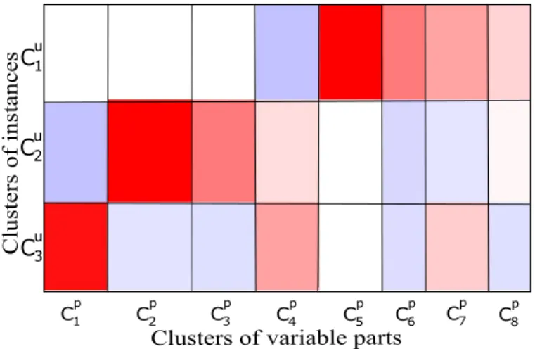
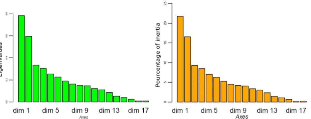
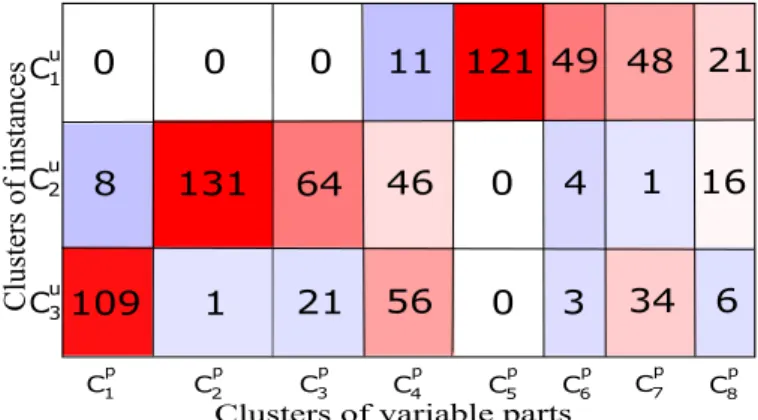
rep-resent the instance clusters while the columns reprep-resent the vari-able part clusters. In each cell, the red color represents an over-representation of the instances compared to the case where the two dimensions are independent and the blue color represents an under-representation. White cells represent empty co-clusters (no association between the corresponding clusters). . . 52 3.2 Histogram of eigenvalues (on the left) and the percentage of

variance captured by the axes in the MCA analysis of Iris (on the right). . . 55 3.3 K-means clustering of the projection of the set of instances

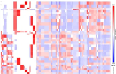
and variable parts. . . 55 3.4 Co-clustering of the Adult data set. Each square represents a

co-cluster. This MODL optimal co-clustering contains 34 × 62 co-clusters. . . 58 3.5 A simplified co-clustering of the Adult data set, with 70% of

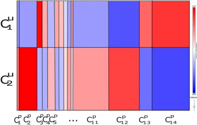
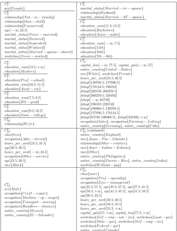
information. The rows represent clusters of instances while the columns represent clusters of variable parts. . . 58 3.6 A simplified co-clustering of the Adult data set, with 2 × 14

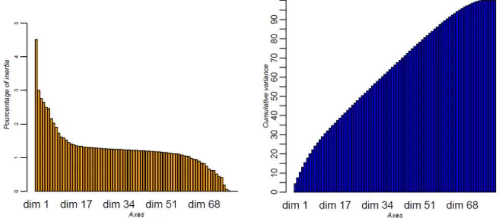
co-clusters. . . 59 3.7 Barplots of the variability (on the left) and the cumulative

information captured by the axes (on the right) in the MCA analysis of Adult. . . 60 3.8 Projection of the set of instances and variable parts, of the

Adult data set, on the first factorial plan. . . 61 3.9 Projection of the k-means centers with k=10 and k=100

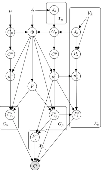
clus-ters, on the first factorial plan. . . 61 4.1 A directed graphical model of the distribution. Parameters

are omitted on this representation for simplicity. . . 79 4.2 A directed graphical model of the full distribution. Variable

related elements have been separated into one plate for qual-itative variables (with Xc as the range of the plate) and two plates for quantitative variables (with Xn as the range of the plates). . . 79 x

(11)

LIST OF FIGURES xi

5.1 Iris: evolution of the criterion values. . . 93

5.2 Iris: the resulting co-clustering. . . 94

5.3 Iris: the co-clustering resulting from the methodology in Chapter 3. . . 95

5.4 Iris: number of clusters of instances (CrossCat). . . 99

5.5 Iris: distribution of the number of instances per cluster (CrossCat). . . 99

5.6 Our model: projection of the Iris flowers. . . 100

5.7 CrossCat: projection of the Iris flowers. . . 100

5.8 Adult: evolution of the criterion values. . . 101

5.9 Adult: the optimal clustering. Each square represents a co-cluster. This optimal co-clustering contains 61 × 72 co-clusters.101 5.10 Adult: cumulative mutual information per co-clustering struc-ture. . . 102

5.11 A clustering of the Adult data set containing 12 × 17 co-clusters. . . 104

5.12 A clustering of the Adult data set containing 2 × 17 co-clusters. . . 104

5.13 Adult: examples of ranking clusters of instances by clusters of variable parts. . . 106

5.14 Adult: comparison of the optimized partition of the variable education_num with the parameter based one. . . . 109

5.15 CensusIncome: the optimized co-clustering. Each square represents a co-cluster. This optimal co-clustering contains 607 × 97 co-clusters. . . 111

5.16 CensusIncome: 12 × 12 co-clusters. . . 111

5.17 CensusIncome: 2 × 12 co-clusters. . . 112

5.18 CrossCat on independent variables. . . 115

5.19 Our co-clustering on correlated variables. . . 115

5.20 CrossCat on correlated variables: the number of clusters of instances and variables. . . 116

(12)

List of Tables

2.1 Examples of co-cluster types. . . 15

3.1 The output of the discretization step on iris, for p=5. . . . 44

3.2 The first 10 instances of the transformed Iris data. . . 45

3.3 The contingency-table representation of Iris. C_ku denotes the kth cluster of instances and C_lp denotes the lth cluster of variable parts. 53 3.4 Table of mutual information of the Iris data co-clustering. . 53

3.5 Composition of the instance clusters.. . . 53

3.6 Composition of the variable part clusters. . . 54

3.7 Confusion table between our clustering and the k-means clus-tering. Ci stands for the ith k-means cluster. . . 56

3.8 Summary of the clusters of instances using k-means. . . 62

3.9 The confusion matrix between the co-clustering and k-means partitions. . . 62

3.10 Composition of the clusters of variable parts in the simplified Adult co-clustering. . . 65

4.1 Data example. . . 69

4.2 A simple data set in its natural representation. . . 73

4.3 Data set from table 4.2 in the observation representation. . . 73

4.4 A binary representation of the data based on the variable parts. . . 74

4.5 Contingency table associated to the co-clustering. Each cell contains the number of observations (see Table 4.3) that fulfill the constraints associated to the corresponding clusters: the instance must be in the instance cluster of the row, while the variable must fulfill one of the conditions associated to the variable parts of the column. The last column and row are marginal counts. On this example, one can see that the co-clustering is revealing a dependency between instances and variable parts in the first two columns as some co-clusters are empty. . . 75

5.1 Iris: number of observations per co-cluster. . . 94

5.2 Iris: mutual information. . . 94

5.3 Iris: the variable parts and their compositions.. . . 95

5.4 Iris: composition of the clusters. . . 96

(13)

LIST OF TABLES xiii

5.5 Adult: composition of the variable part clusters, showing the strong interdependence between the variables education_num and education. The categorical parts delimited by a plus sign (+) are the result of multiple parts that are merged in the optimization step into one. . . 102 5.6 Adult: counts per co-cluster, showing the strong dependence

between the variables education_num and education. . . . . 103 5.7 Adult: composition of the clusters of instances in the 12 × 17

co-clustering (top) and the 2 × 17 co-clustering (bottom). . . 104 5.8 Adult: number of observations per co-cluster in the 12 × 17

co-clustering. . . 105 5.9 Adult: number of observations per co-cluster in the 2 × 17

co-clustering. . . 105 5.10 Adult: content of the co-clusters expressing the correlation

between education and education_num from the simplified 12 × 17 co-clustering. . . 108 5.11 Adult: the optimized number of parts per variable. . . 109 5.12 Adult: examples of the number of observations per part. . . 109 A.1 Adult: partitioning of the variables in the optimal co-clustering.127 A.2 Adult: mutual information of the 12 × 17 co-clustering. . . . 128 A.3 Adult: mutual information of the 2 × 17 co-clustering. . . 128 A.4 Adult: partitioning of the variables in the 12 × 17 co-clustering.131 A.5 Adult: composition of the clusters of variable parts in the

(14)

(15)

Chapter 1 Introduction

Nowadays, the amounts of data collected from different sources, in various formats, and for various application areas is growing not only in the number of objects and attributes, but also in the complexity of the patterns to be ex-tracted from the data. This has led to an increasing need for the development of techniques and tools to assist the analyst in extracting useful information (knowledge), from the rapidly growing volumes of data. The development of such techniques would enable intelligent and automatic analysis, exploration and organization of large and complex data, to extract and understand in-formation. Moreover, with the emergence of connected objects, the volumes of available data and their diversity can only keep growing.

On the one hand, the increasing amount of data and the development of data mining techniques makes knowledge discovery tasks especially interest-ing for large companies, since they allow the data to be considered as a useful resource in the decision-making process. On the other hand, the increasing complexity of the data creates several challenges for the researchers, provided that many existing techniques are not appropriate to analyze large complex data. For example, consider the field of market analysis, where millions of transactions are observed. Data analysis techniques are used to analyze and summarize the information contained within these large data sets and to draw conclusions about the data and the studied objects. The collected data can be anything from demographic descriptors of the customers (age, gender, social class, occupation, education, income) to markers of customer prefer-ences such as ratings. The analysis tools can range from simple analysis tools such as graphical displays such as bar charts and histograms, two-way tables such as contingency tables, and quantile plots (Amant and Cohen 1995) to more complex tools such as applying machine learning techniques (Everitt et al. 2011) to learn a buying pattern or to create a grouping of customers. Finally, the extracted conclusions can be used in recommendation systems.

However, the growing size of data sets has led to an increasing demand for efficient and noise tolerant data summarizing techniques for data com-pression and analysis, while respecting constraints in terms of memory usage and computation time.

(16)

2 CHAPTER 1. INTRODUCTION

1.1 Problem definition and main objectives

The main theme of this thesis is the use of co-clustering in exploratory anal-ysis. Given a data matrix where the rows represent objects and columns represent their features, the goal of a co-clustering technique is to

simulta-neously extract clusters of objects and clusters of features. The co-clustering

techniques try to exploit the interdependence between the objects and their descriptive features to create groups of objects and groups of features or of feature values in a way that best expresses the level of association between these groups. Hence expressing the association between the two sets.

With mixed-type commercial data in mind (such as e-commerce and consumer/product data), we seek a simultaneous clustering technique that would provide an easily exploitable summary of the data. When working with such data, a first level of complexity arises from the properties of the various attributes used to describe each data object, such as the fact that they are categorical or numerical, the cardinality of the domains, and the dependencies that may exist between different attributes. A second level of complexity arises from the fact that these data are considerably large and may have missing values. A third level of complexity arises from the variety of tasks that can be performed to analyze the data and from the existence of several alternative ways to perform each task. Thus, depending on the nature of knowledge one wants to extract, some techniques are more suitable than others.

Our goal is to propose a co-clustering method that handles data with mixed-type attributes, handles missing data, provides easily interpretable clusters and, overall, a good summary of the data and an evaluation measure.

1.2 Outline of the thesis

This manuscript is organized as follows.

• In Chapter 2, we define the problem of co-clustering and explore the existing literature on the subject. In this chapter, we will notice the multitude of solutions, their main differences, advantages and limita-tions.

• In Chapter 3, we propose a new approach for co-clustering mixed-type data. The approach is based on a user defined pre-processing step followed by a value oriented co-clustering technique. In this chapter, we show that the proposed approach enables extracting easily inter-pretable clusters of objects, captures local as well as global dependen-cies between the variables, and that it scales to data sets containing tens of thousands of objects and hundreds of thousands of entries. • Chapter 4 describes a co-clustering model that formalizes the approach

proposed in Chapter 3. The model eliminates the pre-processing phase by simultaneously inferring an optimized partitioning of each variable

(17)

1.3. PUBLICATIONS 3

and performing a co-clustering, by optimizing a Maximum A Poste-riori (MAP) based model selection criterion. The model requires no user parameter and it enables associating values coming from different variables by setting the data matrix entries as the statistical units. • Chapter 5 provides experimental results on synthetic and real-world

data sets. These experiments highlight the main features of the co-clustering model proposed in Chapter 4, some of the possible ways in which a co-clustering model can be exploited, and provide a didactic explanation of how the model works and how it differs from the solution proposed in Chapter 3.

• Finally, in Chapter 6 we draw concluding remarks and highlight pos-sible future perspectives and use cases for the proposed co-clustering model.

1.3 Publications

The work presented in this thesis is the subject of the following publications. 1. The work presented in Chapter 3 has contributed to the paper:

Bouchareb, A., Boullé, M., Clérot, F., and Rossi, F. (2017a). Appli-cation du coclustering à l’analyse exploratoire d’une table de données. In 17ème Journées Francophones Extraction et Gestion des

Connais-sances, EGC 2017, volume RNTI-E-33, pages 177–188.

2. An extended version of Bouchareb et al. (2017a) is the subject of: Bouchareb, A., Boullé, M., Clérot, F., and Rossi, F. (2018a). Co-clustering based exploratory analysis of mixed-type data tables. In Pinaud, B., Gandon, F., Bisson, G., and Guillet, F., editors, Accepted

for publication in Advances in Knowledge Discovery and Management Vol. 8 (AKDM-8). Springer.

3. The work presented in Chapter 4 has contributed to the paper: Bouchareb, A., Boullé, M., Rossi, F., and Clérot, F. (2018c). Un modèle bayésien de co-clustering de données mixtes. In Extraction et Gestion

des Connaissances, EGC 2018, Paris, France, January 23-26, 2018,

pages 275–280.

4. To perform a co-clustering of mixed data, we have extended the Latent Block Models to the case of data containing binary and numerical variables. This extension is not presented in the core of this thesis, but is the subject of:

Bouchareb, A., Boullé, M., and Rossi, F. (2017b). Co-clustering de données mixtes à base des modèles de mélange. In 17ème Journées

Francophones Extraction et Gestion des Connaissances, EGC 2017, 24-27 Janvier 2017, Grenoble, France, pages 141–152.

(18)

4 CHAPTER 1. INTRODUCTION

5. Appendix B contains an extended version of the work published in Bouchareb et al. (2017b). This extended version is the subject of: Bouchareb, A., Boullé, M., Clérot, F., and Rossi, F. (2018b). Model based co-clustering of mixed numerical and binary data. In Pinaud, B., Gandon, F., Bisson, G., and Guillet, F., editors, Accepted for

pub-lication in Advances in Knowledge Discovery and Management Vol. 8 (AKDM-8). Springer.

(19)

Part I

State of the art

(20)

(21)

Chapter 2 Co-clustering for exploratory

data analysis

This chapter gives an introduction to the subject of exploratory data anal-ysis. In particular, we focus on the co-clustering based techniques. The objective is to lay out the motivating backgrounds for the rest of the the-sis by introducing the most commonly known co-clustering techniques, their advantages and drawbacks as well as their domains of application.

This chapter is organized as follows. First, we briefly outline the con-text of exploratory analysis in Section 2.1. Section 2.2 presents the types of data sets we wish to analyze. In Section 2.3, we give a brief overview of discretization methods and their use for homogenizing the data as well as some of the most commonly used multivariate data description techniques, namely clustering and dimensionality reduction techniques. In particular, we illustrate the various choices involved in the process of data clustering, starting from the choice of the variables to the choice of the number of clus-ters, and introduce dimensionality reduction as a commonly used technique for data visualization and for association extraction. Section 2.4 introduces co-clustering as an extension of the clustering problem, the most commonly used co-clustering techniques, the types of structures they extract and their domains of applicability. In particular, we will distinguish between row and column based approaches (Section 2.5) and value based approaches (Sec-tion 2.6). Sec(Sec-tion 2.7 summarizes the main limita(Sec-tions of these methods and sets the motivation for the next chapter.

2.1 Introduction

The amount of data available nowadays is too large to process manually. Hence, one of the most common activities of the data analyst consists in trying to extract some essence information from an abundance of data. This urge for information extraction is particularly present in the industrial context where data is abundant and the necessity to exploit information be-comes pressing. For example, companies like Orange hold information about their clients, their purchase history, and their preferences. With a large

(22)

8 CHAPTER 2. CO-CLUSTERING FOR EXPLORATORY ANALYSIS

ber of clients and ultimately a large number of attributes, exploratory data analysis becomes an essential tool in decision making. In particular, there is a need to use the collected data about users and their preferences (such as age, the products purchased, ratings, . . .) to create reliable recommenda-tions for a set of clients of interest or make general marketing policies like offering discounts on the products generally purchased together.

Data analysis tools differ in their objectives and underlying hypothesis. For example, these techniques are usually divided into two main types: su-pervised and unsusu-pervised methods. In the susu-pervised learning approach, also called predictive analysis, the goal is to learn a mapping from a set of inputs x to a set of outputs y, given a so called training set of labeled input-output pairs D = {(xi, yi)}Ii=1, where I is the size of the training

set (Murphy 2012). These techniques are called predictive because, ulti-mately, the goal is to predict, using the learned mapping, the output value

yj for new unlabeled values xj. Examples of supervised methods include: neural networks, simple and multiple linear regression, and support vector machines (see: Maimon and Rokach (2010), Bishop (2006), Schölkopf and Smola (2002)).

The second main type of data analysis techniques is the unsupervised learning approach where only a set of unlabeled inputs D = {xi}Ii=1 is

given, and the goal is to find interesting structure in the data (which is sometimes called knowledge discovery (Murphy 2012). The work presented here falls in this context of information extraction and knowledge discovery in databases. As Maimon and Rokach (2010) put it:

Knowledge Discovery in Databases (KDD) is an automatic, exploratory analysis and modeling of large data repositories. KDD is the organized process of identifying valid, novel, useful, and understandable patterns from large and complex data sets.

Therefore, the goal is to find interesting patterns by organizing and sum-marizing the data in a way that extracts humanly understandable

conclu-sions. However, the term "interesting" is not well defined in the sense that

the types of expected patterns are either unknown or task dependent, and that there is no natural error metric as in the case of predictive analysis, for example. These features make descriptive analysis a more complex task since the problem is not well defined and lacks a universal evaluation measure. On the other hand, these same features make descriptive analysis a flexible task and data dependent tool as there are less performance constraints and the analyst simply uses a set of discovery tools in order to make statements about the data and describe what it is or what it shows, through simplifi-cation. Instead of computing an error metric, the questions to be asked in an exploratory analysis context are of the type: have the right tools been chosen with respect to the task at hand, have the tools been used correctly, how credible are the statements and conclusions.

(23)

2.2. DATA REPRESENTATION 9

subset of unsupervised methods, to lay out the motivational backgrounds for the work presented in this thesis, which falls in the framework of extracting relevant patterns from the data.

The process of performing an exploratory analysis encompasses a wide variety of choices that need to be made in order to extract any knowledge from data. The extracted knowledge, if any, is the composite result of all the choices. The first of these choices is to define what can be considered as "data", both in the objective sense and with respect to the type of knowl-edge we want to extract. The second choice concerns the definition of the exploratory analysis tools and the type of patterns one is seeking.

2.2 Data representation

Generally, the data D can be of any type and form. However, for easy manipulation of raw data, the data to be analyzed is usually represented as a set of points (called objects or instances) in a K-dimensional space of features (called variables). That is, data are generally represented in a rectangular table with I rows for the set of instances and K columns corresponding to the variables.

Choosing the instances and variables to analyze is a crucial phase and has an important influence on the results. This choice has to take into account the aim of the study. In particular, the variables have to describe the phenomenon being analyzed (Anderberg 1973). For example, in census data, the instances are individual persons and the features could be any thing from age, income, number of family members, marital status, . . ., to

level of education and household electricity consumption. In market analysis,

when modeling purchasing patterns, the data can consist of a binary matrix where each column represents a product, each row represents a client, and an entry is equal to 1 if the corresponding product was purchased by the corresponding client.

Regardless of the application domain, let X = (xij)1≤i≤I, 1≤j≤K be the

matrix representation of the data containing the observed data values where

I is the number of instances, K is the number of variables, and the entry xij =v says that the value of the jth variable is v for the ith instance.

Depending on the measured feature, a variable can be:

• categorical (also referred to as qualitative) to designate a variable for which the space of values is a finite set of un-ordered values,

• numerical (also referred to as quantitative) to designate a variable for which the values can be ranked in order and are subject to meaningful arithmetic operations.

Depending on the nature of the variables, data can be uni-type or mixed. Uni-type data is numerical when all variables are numerical and categorical when all variables are categorical (note that binary variables are a special

(24)

case of the categorical type but with only two categories). We refer to mixed data when both types of variables are present.

The goal of this thesis is to introduce an exploratory analysis technique for large and mixed data sets. More precisely, our goal is to analyze data containing millions of values (up to 10 millions) while providing easily in-terpretable results. But first, in the coming sections, we introduce the most commonly used exploratory analysis techniques. The literature shows that these techniques are mostly adapted for uni-type data and their performance can be limited when the data is large and complex in the sense that they would extract global summaries about the instances or variables but can miss subtle patterns like local cross-dependencies.

2.3 Standard exploratory analysis techniques

Simple exploratory analysis tools include graphical displays for examining the shape of the sample distribution such as bar charts and histograms, two-way tables such as contingency tables, and quantile plots (Amant and Cohen 1995). More complex exploratory analysis tools include discretization and scale conversions (Maimon and Rokach 2010, Liu et al. 2002), cluster analysis (Everitt et al. 2011), and correspondence analysis (Greenacre and Blasius 2006, Beh and Lombardo 2014). Here, we give a brief overview of these techniques.

2.3.1 Discretization

Discretization is a data processing procedure that transforms quantitative data into qualitative data and can also be useful if the variable is categorical but with too many categories or highly varying frequencies. This process is an important task of the data pre-processing, not only because some learning methods do not handle numerical variables, but also because discrete data and especially intervals are cognitively easier to apprehend and are often more relevant for a human interpretation than the actual values a variable takes (Liu et al. 2002). In addition to easier interpretation, the computation time can be significantly reduced when the data is transformed to a finite set of categories instead of containing a hypothetically infinite number of values as is the case for a numerical variable (Ho and Scott (1997), Frank and Witten (1999), Catlett (1991)). This computation time reduction is especially relevant if the cutting points are relevant to the learning problem at hand (Liu et al. (2002), Mittal and Cheong (2002)). Finally, in addition to harmonizing the nature of the data if it is heterogeneous, discretization can reveal complex relations between the variables to the learning process (Chen et al. (2017), Friedman and Goldszmidt (1996)). However, two key problems in association with discretization are how to select the number of intervals, and how to perform the discretization (see Maimon and Rokach (2010) and Liu et al. (2002) for more details on discretization methods).

(25)

2.3. STANDARD EXPLORATORY ANALYSIS TECHNIQUES 11

Examples of discretization techniques include width and equal-frequency discretization (Liu et al. 2002, Anderberg 1973), entropy and minimum description length based discretization (Friedman and Goldszmidt 1996, Fayyad and Irani 1993).

2.3.2 Clustering

Clustering is by far the most widely used exploratory analysis technique. The goal of clustering is to find a summary of the data in the form of groups of instances. That is to find an optimal grouping for which the instances within each cluster are similar, but the clusters are dissimilar to each other. The similarity between the instances is measured using all the measured attribute values. Hence, overall, the objects within the same cluster are assumed to behave similarly with respect to all the measured attributes.

However, in spite of its wide use, data clustering is a challenging task as it involves many choices (Jain et al. 1999). For example, aside from the data representation, the major choices in performing a cluster analysis include the choice of the variables (Anderberg 1973), the structure and type of the desired clustering (hierarchical, partitioning, density based, grid based, hard, fuzzy, . . .). Furthermore, many techniques require choosing a similarity or dissimilarity measure between the items to cluster. Other clustering methods use a within- and between-cluster variability as a preliminary measure for clustering optimality (Rencher 2002). Moreover, depending on the type of clustering and the similarity measure, a variety of different methods can be used to perform a data clustering. Besides, very often, the number of clusters need to be specified and there is a multitude of cluster evaluation criteria (see Jain et al. (1999), and Maimon and Rokach (2010) for a comprehensive review of data clustering methods).

Because of the existence of several alternative ways to perform a cluster-ing, and given the lack of consensus on a natural metric to evaluate a clus-tering, finding an appropriate data clustering is a complex and challenging task. Furthermore, another level of complexity arises when the data con-tains mixed-type variables since most clustering techniques are designed for uni-type data. To cluster mixed data, one of the most common approaches is converting the data set to a single data type, and applying standard clus-tering technique to the transformed data (Foss et al. 2016). However, this raises the same issues raised above for discretization (Section 2.3.1), namely how to select the number of intervals and how to perform the discretization. Examples of clustering techniques include: K-means, self-organizing maps, spectral clustering, density based clustering (Jain et al. 1999).

2.3.3 Dimensionality reduction

A common problem encountered by most of the traditional clustering tech-niques is the curse of dimensionality (Maimon and Rokach 2010) which refers to the fact that increasing the number of attributes describing the objects

(26)

quickly leads to significant degradation of the performance of object cluster-ing techniques (Murphy 2012). In fact, accordcluster-ing to Maimon and Rokach (2010), it has been estimated that, as the number of dimensions (variables) increases, the number of instances (sample size) needs to increase exponen-tially in order to have an effective estimate of multivariate densities. To minimize the effect of high number of variables, dimensionality reduction techniques have been proposed.

Dimensionality reduction is a set of non-invertible mappings of data to a lower dimensional space (Maimon and Rokach 2010, Cunningham and Ghahramani 2015). The underlying hypothesis is that although raw data is

represented in a high dimensional format, the information contained in the data can be explained in a lower dimensional space. The most commonly

known dimensionality reduction techniques are linear, projection based, mappings where the goal is to find an optimal low-dimensional projection of the data (Sun et al. 2009). Namely, these techniques try to maximize the data variance captured by the low-dimensional projection, or equivalently to minimize the reconstruction error of the original data from projected data.

Examples of these commonly used techniques include principal compo-nent analysis (PCA) for numerical variables and multiple correspondence analysis (MCA) for categorical variables (Rencher (2002), Maimon and Rokach (2010)). Ultimately, the goal of these techniques is to uncover the associations between the objects and the features. That is to find the princi-pal dimensions that capture the most variance possible, allowing for lower-dimensional description of the data (Saporta 2006). Other examples of linear mapping based dimensionality reduction techniques include Fisher’s linear discriminant analysis LDA (Fisher 1936, Bishop 2006) where the purpose is to project the data such that the separation between classes is maximized. Non linear techniques include the non-negative matrix factorization NMF (Lee and Seung 2011), detailed in Section 2.5.2 (see la Torre (2012) and Scholkopf and Smola (2001) for examples of other nonlinear techniques).

Thanks to their capability of providing a description of the data in a lower dimensional space, these techniques have been shown to be particu-larly useful when the observed raw data is high dimensional data, but the intrinsic information included in the data can be visualized and explained in a lower dimensional subspace. Hence, they have been extensively used for visualizing high dimensional data. A common practice is thus to combine dimensionality reduction with a clustering technique where only the lower dimensional representation of the data is clustered.

However, despite their popularity, the usage of dimentsonality reduction methodologies for overcoming the obstacle of high dimensionality has several drawbacks (Maimon and Rokach 2010). First, the assumption that a large set of input features can be reduced to a small subset of relevant features is not always true. In some cases, all the features (or at least a significant ma-jority) are of equal importance to the information contained in the data, and removing some features will cause a significant loss of important information. Second, in some cases, even after eliminating a set of irrelevant features, the

(27)

2.4. CO-CLUSTERING 13

researcher is left with relatively large numbers of relevant features which means that a post-analysis method (such as clustering) is required to actu-ally visualize and analyze the data. Furthermore, these methods have been shown to be noise sensitive and, although they provide interesting results when applied to relatively small data sets, they stay of limited use for the analysis of large data sets.

2.4 Co-clustering

Most of the data analysis literature focuses on the problem of clustering for structure extraction or a combination of a clustering technique with di-mensionality reduction. However, the data can contain patterns that may be hard to capture using a traditional clustering approach. For example, consider the dyadic data of documents and words represented by a matrix, whose rows correspond to documents, columns correspond to words, and entries correspond to the counts of the words in documents. Given such data, one can perform a clustering of documents or words (depending on the goal of the analysis) using a traditional clustering approach. However, such one-sided clustering might fail to discover subtle patterns of the data. For example, some words may only appear in some sets of documents and inversely some documents may be clustered together because they contain specific words, which means that the data matrix exhibits a strong depen-dency structure between groups of words and groups of documents. In order to extract such patterns, one approach that has gained increasing attention, over the years, is the simultaneous clustering of the set of rows and the set of columns of the data matrix (also called co-clustering, cross-clustering or bi-clustering).

Proposed by Good (1965), then by Hartigan (1975), as an extension of standard clustering, co-clustering is a data mining technique that aims to jointly cluster both the object and feature dimensions simultaneously. Thus, taking advantage of the duality and interdependence between the set of objects and the set of variables. Whereas the principle of standard clustering is that of grouping objects that are similar with respect to the set of variables, the task of co-clustering is to simultaneously find groups of similar objects (with respect to the variables) and groups of similar variables (with respect to the objects).

The main advantage of these techniques is that they provide a powerful tool for extracting the existing dependencies between the instances and their descriptive variables, which enhances the interpretability of the clusters of in-stances using the clusters of variables and vice-versa. In some sense, this can be seen as a dimensionality reduction that operates both on the dimension of instances and the dimension of variables. Co-clustering is, for example, an interesting technique to consider in market analysis where a customer is represented by a vector, across a list of products (and vice-versa). In this case, the analyst can be more interested in identifying the subsets of cus-tomers that tend to buy the same subset of products and which products

(28)

they buy, than simply trying to group customers (or products) based on buying/selling patterns, which is the task accomplished by regular cluster-ing. In contrast to a regular clustering technique, co-clustering customers and purchased products allows to discover the items of interest for a partic-ular client/set of clients and thus build more precise recommendations and efficient promotions and sales strategies.

Another advantage of these techniques is their capability of summarizing a data matrix where the summary matrix is the matrix of co-clusters (also called blocks). The matrix of co-clusters is, in some sense, the essence of the data. This point of view is particularly interesting in exploratory data analy-sis where replacing the original, often large, data matrix by the considerably smaller matrix of co-clusters can facilitate analysis.

2.4.1 Definition

Let X be a data matrix as defined in Section 2.2 and let U be the set of I objects and X the set of K variables. Formally, most co-clustering methods are defined by a mapping ˆC_U : U → {C₁i, . . . , C_gi} from the set of instances to groups of instances and a mapping ˆCX : X → {C1v, . . . , Cmv} from the set of variables to groups of variables, where g and m are the number of clusters of instances and the number of clusters of variables, respectively. The intersection of a group of instances and a group of variables forms a co-cluster which can be seen as a sub-matrix of the instance-variable matrix. The challenge of co-clustering is to extract a structure in the form of

homogeneous blocks. The nature of such structure and the definition this homogeneity condition depend on the co-clustering method and can be

char-acterized by how the rows and columns are assigned to clusters, and by the input data-type.

2.4.2 The homogeneity condition

The homogeneity condition, defined by the content of the co-cluster, varies from one method to another. Most clustering methods try to find co-clusters with constant values per co-cluster or, in the probabilistic context, co-clusters whose elements are issued from the same probability distribution. More generally, the literature distinguishes between co-clustering methods with respect to the content of the co-clusters (non exclusive examples are given in Table 2.1):

• Co-cluster with constant values (Table 2.1a),

• Co-cluster with constant values per row (Table 2.1b), • Co-cluster with constant values per column (Table 2.1c), • Co-cluster with coherent evolution over the rows (Table 2.1d), • Co-cluster with coherent evolution over the columns (Table 2.1e),

(29)

• Co-cluster with coherent evolution over both rows and columns (Ta-ble 2.1f),

• Co-cluster with coherent values, obtained via a multiplicative or ad-ditive relationship between the row and column values or following a complex mathematical model that depends on the co-cluster. For example, in Table 2.1g, an element bkl of the co-cluster is given by the additive model b_kl = µ+α_k +β_l where µ = 5, α = (4, 2, 3) and

β = (1, 5, 3). 1 1 1 1 1 1 1 1 1 (a) 1 1 1 3 3 3 2 2 2 (b) 1 3 2 1 3 2 1 3 2 (c) 1 3 9 5 20 80 3 15 75 (d) 1 6 3 5 24 9 25 96 18 (e) 1 3 9 3 15 75 5 20 80 (f) 10 19 12 8 12 10 9 13 11 (g)

Table 2.1 – Examples of co-cluster types.

The set of blocks form a structure. However, many different structures exist in the literature as each co-clustering method searches for a specific structure of blocks. In the following, we will focus on the methods that provide co-clusters with constant or coherent values to explore the most commonly extracted structures.

2.4.3 The co-clustering structure

The co-clustering structure is defined by the relationship between different clusters. More precisely, let us distinguish four types of methods.

1. Partitioning methods: the clusters define a partition of non empty non intersecting subsets that span the set of possibilities (the full set of I instances and the full set of K variables). In such cases, the co-clusters can be formed of the cartesian product of a partition of rows and a partition of columns (this is known as block clustering).

2. Overlapping clustering: each instance and each variable can belong to multiple clusters.

3. Nested clustering: the co-clusters can be defined by intersecting clus-ters. However, unlike overlapping clusters, if two clusters intersect, then one of them is necessarily a subset of the other (Mechelen et al. 2004). An example of nested clustering is given by the hierarchical co-clustering where the row and column clusters are defined by the cartesian product of a hierarchy of rows and a hierarchy of columns or a hierarchy of the I × K values in the data matrix.

4. Other types of structures include sets of subgroups. That is, a co-cluster is defined by a subgroup of instances and a subgroup of variables or in the case of value clustering, a subgroup of the I × K values.

(30)

However, in this case, not all rows/columns or values are required to belong to clusters.

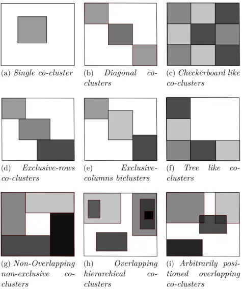
Madeira and Oliveira (2004) provide a more detailed and general classifi-cation of these structure types found in gene expression co-clustering meth-ods as shown in Figure 2.1. The details of these structures are as follows.

(a) Single co-cluster (Figure 2.1a), defined by one group of instances and one group of variables.

(b) Exclusive row and column co-clusters (Figure 2.1b): the assumption is that there exists a permutation of the rows and columns of the data matrix after which the co-clusters form rectangular diagonal blocks. This corresponds to a particular case of partition of the rows and a partition of the columns in Figure 2.1c.

(c) Non-overlapping co-clusters with checkerboard structure (Figure 2.1c): there exists a permutation of the matrix rows/columns after which the co-clusters form rectangular contiguous blocks. This corresponds to a partition of the rows and a partition of the columns.

(d) Exclusive-rows co-clusters (Figure 2.1d): this corresponds to co-clusters defined by a partition of the rows and overlapping co-clusters of columns.

(e) Exclusive-columns clusters (Figure 2.1e): this corresponds to co-clusters defined by overlapping co-clusters of rows and a partition of the columns.

(f) Non-Overlapping co-clusters with tree structure (Figure 2.1f). (g) Non-Overlapping non-exclusive co-clusters (Figure 2.1g).

(h) Overlapping co-clusters with hierarchical structure (Figure 2.1h): hi-erarchical partitioning of the I × K values of the data matrix.

(i) Arbitrarily positioned overlapping co-clusters (Figure 2.1i): a set of possibly overlapping subgroups of the I × K values.

2.4.4 The co-clustering strategy

In order to extract the desired co-clustering structure, many co-clustering strategies have been studied in the literature. The most commonly followed strategies include the following.

• Clustering rows then columns independently, using a standard clus-tering technique, then simultaneously analyzing the results to fetch for a co-clustering structure (Lerman and Leredde 1977, Madeira and Oliveira 2004).

(31)

(a)Single co-cluster (b) Diagonal co-clusters (c)Checkerboard like co-clusters (d) Exclusive-rows co-clusters (e) Exclusive-columns biclusters

(f) Tree like

co-clusters (g)Non-Overlapping non-exclusive co-clusters (h) Overlapping hierarchical co-clusters

(i) Arbitrarily posi-tioned overlapping co-clusters

Figure 2.1 – Examples of co-clustering structures.

• Performing a standard clustering technique on the rows (resp. columns) then a standard clustering technique on the columns (resp. rows) while taking into account the first clustering results (Tishby et al. 1999). Examples of these methods include the Coupled Two-way Clustering (Getz et al. 2000), which performs a bi-clustering by al-ternating one-dimensional clustering algorithms, and the Interrelated Two-Way Clustering algorithm (Tang et al. 2001) that combines the results of one-way clustering(s) on both dimensions of the data matrix in order to produce co-clusters.

• Simultaneously clustering the rows and columns of data matrix (Go-vaert 1983; 1995, Kluger et al. 2003, Yoo and Choi 2010, Shan and Banerjee 2008).

In the coming sections, we introduce some of the most commonly known co-clustering methods to emphasize the richness of the field and to illustrate the different types of approaches. In particular, we will focus on the ap-proaches that perform a simultaneous clustering of the rows and columns.

(32)

18 CHAPTER 2. CO-CLUSTERING INSTANCES × VARIABLES

For a full survey of the co-clustering methods, readers are refered to: Charrad and Ahmed (2011), Tanay et al. (2005), Madeira and Oliveira (2004), Brault and Mariadassou (2015), Brault and Lomet (2015), Pontes et al. (2015), and Padilha and Campello (2017).

2.5 Simultaneous clustering of the instances

and variables

The simultaneous clustering problem has been shown to be an NP-hard problem (Tanay et al. 2002). In particular, an exhaustive search of the space of solutions is infeasible, which requires most of the existing meth-ods to base their search on heuristic optimization procedures. The use of a suitable co-cluster evaluation measure and the development of an effective search heuristic are two crucial factors for finding significant co-clusters with reasonable resources. Pontes et al. (2015) reviews a large number of biclus-tering approaches used in gene expression analysis and classifies them into two categories: biclustering algorithm based on evaluation measures, and non metric-based biclustering algorithms.

In this section, we introduce some of the most common approaches to perform a simultaneous clustering of the instances and variables in a data table. In particular, we will distinguish between cost function, linear algebra, and parameter identification based methods.

2.5.1 Deterministic cost function based co-clustering

In the literature, many co-clustering algorithms propose to optimize an ob-jective function called co-cluster evaluation function. Most of theses objec-tive functions try to summarize the original data matrix X by a new smaller matrix ˆX = (ˆxkl)1≤k≤g,1≤l≤m containing a summarized representation of

the blocks (such as the mean or median value), or by some reconstructed data matrix ˆX = (ˆxij)1≤i≤I,1≤j≤K of the same size as X but with constant

entries within each block.

Deterministic objective function based algorithms try to define the couple of mappings from the instances to instance clusters and from the variables to variable clusters that optimize a co-cluster quality measure that characterizes the difference between the original data X and the co-clustered data ˆX. Hartigan’s direct clustering

When Hartigan (1972) introduced co-clustering as "direct clustering", he proposed to simultaneously cluster the rows and columns of a data table. The algorithm seeks co-clusters with constant values or low within-block variance. To do this, he approximates the original data matrix by the matrix ˆX that minimizes the sum of squared residues. As a result, the values within each co-cluster are identical. The quality of a co-cluster B_kl = (C_ki, C_lv)

(33)

19

(defined by the cluster C_ki of rows and the cluster C_lv of columns) is given by the within-co-cluster variance:

C(C_ki, C_lv) = X i∈Ci k,j∈C v l (xij − ˆxij)2.

Given a desired number of bi-clusters B, the proposed algorithm is a di-vide and conquer type algorithm that starts with the entire data in a single block then at each iteration finds the row split or column split that pro-duces the largest reduction of the total within-block variance. The splitting continues until the reduction of block variance is not greater than a given threshold. The algorithm results in a tree like hierarchical clustering of rows and columns of the data matrix. The quality of a co-clustering is measured by the overall variance of the B bi-clusters:

C(X, ˆX) = B X b=1 I X i=1 K X j=1 (xij− ˆxij)2.

However, the main drawback of this successive splitting heuristic is that partitions cannot be reconsidered once they have been split. Hence, the final hierarchical clustering can miss some quality biclusters due to premature division of the data matrix. Also, the number of desired co-clusters need to be specified.

One block at a time using the Cheng and Church Algorithm

Cheng and Church (2000) were the first to propose a co-clustering algorithm for gene expression data. The approach uses a measure called Mean Squared Residue (MSR) as measure of co-cluster quality and a greedy algorithm for co-cluster extraction. In particular, the residue of an element xij to block

B_kl = (C_ki, C_lv) is defined as: xij − xi,Cv l − xC_ki,j +xC_ki,C_lv, where x_Ci k,C v l = 1 |Ci k||C v l| P i∈Ci k,j∈C v l

xij is the average of all entries in the block Bkl, xi,Cv l = 1 |Cv l| P j∈C_lv

xij is the mean of all entries in row i whose columns belong to C_lv, x_Ci k,j = 1 |Ci k| P i∈Ci k

xij is the mean of all entries in col-umn j whose rows belong to cluster C_ki, and {|C_ki|, |C_lv|} are the cardinalities of C_ki and C_lv respectively.

For a block Bkl, the goal is to find a sub matrix defined by the couple of groups(C_ki, C_lv)that minimizes, up to a certain threshold, the mean squared residue defined as:

C(C_ki, C_lv) = 1 |Ci k||Clv| X i∈C_ki,j∈C_lv (xij − xi,Cv l − xC_ki,j+xC_ki,C_lv) 2_.

(34)

This mean squared residue measures the level of coherence within the co-cluster as the difference between the observed values xij and the expected values predicted from the corresponding row mean, column mean and bi-cluster mean (Madeira and Oliveira 2004).

The approach uses a greedy iterative search algorithm for rows and columns suppression while minimizing the objective function C up to a given threshold. The algorithm produces one co-cluster at a time (as in Figure 2.1a) and is composed of two stages. In the node (row or column) deletion stage, the algorithm starts with one co-cluster containing the original data matrix then proceeds in iteratively removing rows and columns to achieve the largest decrease of the score while keeping its value under a threshold value. This requires the computation of the scores of all the sub-matrices that may be the consequences of any row or column removal, before each choice of a row/column removal can be made. Once the threshold is reached, the second stage consists of adding rows and columns back to the block if this can be done without increasing the score. After each co-cluster is pro-duced, the elements corresponding to the co-cluster are replaced with ran-dom numbers, then the same procedure is applied on the modified matrix to generate another, possibly overlapping, co-cluster until the required number of co-clusters is reached. Within a co-cluster, the low mean squared residue condition enables extracting co-clusters with coherent values and also con-stant values in some cases. The final extracted structure would reassemble to that in Figure 2.1i.

The algorithm presents several drawbacks, the most important of which is the use of a threshold parameter for rejecting solutions, which is dependent on each data set. Also, the algorithm produces only one co-cluster at a time and as the algorithm proceeds, the random numbers used as replacements for the co-clusters can interfere with the future discovery of co-clusters, es-pecially ones that overlap with the discovered ones which is addressed by Yang et al. (2003). Yang et al. (2003) propose an algorithm called FLex-ible Overlapped biClustering (FLOC) that simultaneously produces B co-clusters whose mean residues are all less than a predefined constant, without the impact of random interference.

Extracting B-blocks simulatenously

Cho et al. (2004) also use squared residue measures similar to those of Har-tigan (1972) and Cheng and Church (2000) in k-means like co-clustering called Minimum Sum-Squared Residue Coclustering (MSSRCC) for homo-geneous block extraction. An homohomo-geneous block is defined by a sub matrix having low average square residues. For every element xij that may belong to co-cluster B_kl, they define two measures for co-cluster quality:

HBkl = (hij)1≤i≤I,1≤j≤K where hij =xij− xC_ki,C_lv, and

(35)

21 where x_Ci k,C v l, xi,C v

l and xCki,j are as defined above. For both measures, they propose an algorithm to minimize the total squared residues:

||H||2₂ = g X k=1 m X l=1 X i∈Ci k,j∈Clv h2_ij.

The first score measures the sum of squared differences between each entry in the co-cluster and the mean of the co-cluster, producing co-clusters with low variance or constant values (as in Hartigan (1972)). The second score measures the sum of squared differences between each entry in the co-cluster and the corresponding row mean and the column mean, while counting for the co-cluster mean for symmetry (as in Cheng and Church (2000)). For co-cluster extraction, the authors propose two iterative algo-rithms that monotonically decrease the objective functions and converge to a local minimum.

The main difference with Cheng and Church (2000) is that Cho et al. (2004) extract B co-clusters simultaneously while Cheng and Church (2000) extracts one co-cluster at a time. Cho and Dhillon (2008) provide specific strategies to enhance the performance of the MSSRCC. For example, like or-dinary k-means-type clustering algorithms, the approach suffers from being trapped in local minima and generating empty clusters. Cho and Dhillon (2008) try to resolve these problems by adopting an incremental local search (LS) strategy, where incremental moves of rows and columns among clusters are performed in order to decrease the objective function value. Also, differ-ent data pre-processing transformations and cluster initialization strategies are investigated. Anagnostopoulos et al. (2008) propose a generalization of this approach that minimizes a p-norm of the residue matrix H = (hij).

The CRO methods

In the same context of cost function opitimization, Govaert (1983) proposes three algorithms: Crobin, Croeuc and Croki2 for binary, continuous and contingency data. Denote z₍_I×g₎, w₍_K×m₎ and ˆX₍_g×m₎ the partition of rows, the partition of columns and the summary matrix. The algorithms alternate between finding the row partition and finding the column partition until the co-clustering criterion reaches a local optimum.

For binary data, the Crobin algorithm searches for homogeneous blocks (blocks with majority of ones or majority of zeros) by optimizing the crite-rion: C(z, w, ˆX) = ||X − z ˆXwt||1 = g X k=1 m X l=1 X i∈Ci k,j∈Clv |xij − ˆxkl|, where ˆX = (ˆxkl)1≤k≤g,1≤l≤m and ˆxkl ∈ {0, 1}.

For continuous data, the Croeuc algorithm uses alternated k-means al-gorithm to minimizes the squared euclidean distances between the elements

(36)

in the block B_kl and its characterizing value ˆx_kl:

C(z, w, ˆX) =||X − z ˆXwt||2 = g X k=1 m X l=1 X i∈C_ki,j∈C_lv (xij− ˆxkl)2.

It is worth noting that these algorithms optimize a criterion that is data-type dependent and that their best bet is to achieve a local optimum of the objective function. Furthermore, the number of clusters of rows and the number of clusters of columns need to be specified. The Croki2 algorithm will be addressed in Section 2.6.1.

2.5.2 Linear algebra and matrix reconstruction based

co-clustering

While the methods introduced above try to optimize the difference between the original data matrix and a summary data matrix, other co-clustering methods focus on decomposing the original matrix to extract associated clus-ters. Among these techniques, we mention those based on latent matrices like Non-negative Matrix Factorization (NMF), and those based on apply-ing a dimensionaliy reduction procedure followed by a standard clusterapply-ing technique.

Matrix reconstruction based co-clustering

Matrix reconstruction based methods try to re-write the optimization (co-clustering) problem in the form of matrix approximation problem, and use matrix factorization (Lee and Seung 2011, Yoo and Choi 2010) to fetch for co-clusters. These algorithms include non-negative matrix factorization (NMF), non-negative tri-factorization (NTF) and non-negative block value decomposition (NBVD).

Non-negative matrix factorization (NMF) searches for the decomposition of a non negative matrix X into a product of two non negative latent matrices that are used for row and column clustering. For example, Lee and Seung (2011) optimize a cost function that characterizes the difference between the original matrix X₍_I×K₎ and the product of two matrices z₍_I×g₎, and wT₍_K×g₎ (T is the transpose). The proposed cost function is either the least square euclidean distance or a generalized divergence measure D of X from zwT

argmin z≥0,w≥0 ||X − zwT||2, or argmin z≥0,w≥0  D(X||c=zwT) = X i,j (xijlog xij cij − xij+cij)  ,

where ||.|| is the Frobenius matrix norm. Iterative minimization algorithms are used to find local minima and are based on multiplicative updating rules.

(37)

23

Given the latent matrices z and w, the clustering of rows can be per-formed by considering the columns of z as row cluster centroids and the ith row of the data matrix X can be associated to the centroid ci (i.e., to its corresponding cluster) which gives the maximum contribution in the linear combination

ci =argmax k

wki,

and inversely for obtaining clusters of columns (Buono and Pio 2015). Buono and Pio (2015) note that this basic NMF provides only casual

clustering and that, to obtain a solution that guarantees a real clustering

interpretation, additional orthogonality constraints on z and/or w should be imposed as in Ding et al. (2006). In Ding et al. (2006), the Frobenius based optimization problem is modified to generate a clustering of rows, by imposing the orthogonality constraint on w (wwT =1, the identity matrix).

In the same manner, a clustering of columns can be achieved by imposing an orthogonality constraint on z (zTz=1).

To perform simultaneous clustering of rows and columns, orthogonality constraints over z and w need to be met simultaneously (solving the op-timization problem under the constraints wwT = 1 and zTz = 1). This

condition is too restrictive, according to Buono and Pio (2015). Further-more, under this double orthogonality constraint, the solutions result in a rather poor low-rank approximation of the data matrix X (always according to Buono and Pio (2015)). Hence, for better approximation, a third latent matrix can be introduced, to create non-negative tri-factorization (NTF), which allows the low-rank approximation to remain accurate, while a soft-orthogonality of z and w is maintained (Buono and Pio 2015).

Non-negative tri-factorization algorithms are similar to NMF except they use only the Frobenius norm and they search to decompose X into the prod-uct z ˆXwT of three latent matrices where ˆX is the non negative summary

matrix and the two binary matrices z and w are for rows and columns classifi-cation respectively (Yoo and Choi 2010). Just like NMF, the tri-factorization algorithm converges to a local minimum.

Non-negative block value decomposition (NBVD) has the same goal as the NTF which is factorizing the data matrix into three latent matrices but uses fuzzy classification matrices for the rows and columns (Long et al. 2005). The algorithm converges to a local minimum by iteratively updating the decomposition matrices using a set of multiplicative updating rules.

Note that these methods apply only to numerical non negative matrices. Also, the NMF approach requires the number of row and column clusters to be the same while NTF allows for the numbers of clusters to differ. However, in both cases, the number of clusters need to be specified. Note also that the Croeuc, Crobin and Croki2 algorithms we mentioned earlier for continuous, binary and contingency data (Govaert 1983) can be reformulated as matrix decomposition algorithms.

A regularized approach of instances x variables co-clustering for exploratory data analysis

THÈSE DE DOCTORAT

Université Paris 1 panthéon-Sorbonne

Aichetou Bouchareb

Docteur

Université Paris 1 panthéon-Sorbonne

A regularized approach of instances

×

variables co-clustering for exploratory

data analysis

Abstract

Résumé

Contents

Contents

List of Figures

List of Tables

1 Introduction

I

State of the art

5

2 Co-clustering for exploratory data analysis

II

Contributions

39

3 Co-clustering mixed data

4 A new co-clustering model for mixed type data

5 Experimental results

6 Conclusion

Appendices

A Adult: details of the co-clustering results

B Model based mixed data co-clustering

List of Figures

List of Tables

Chapter 1

Introduction

1.1

Problem definition and main objectives

1.2

Outline of the thesis

1.3

Publications

Part I

State of the art

Chapter 2

Co-clustering for exploratory

data analysis

2.1

Introduction

2.2

Data representation

2.3

Standard exploratory analysis techniques

2.3.1

Discretization

2.3.2

Clustering

2.3.3

Dimensionality reduction

2.4

Co-clustering

2.4.1

Definition

2.4.2

The homogeneity condition

2.4.3

The co-clustering structure

2.4.4

The co-clustering strategy

2.5

Simultaneous clustering of the instances

and variables

2.5.1

Deterministic cost function based co-clustering

2.5.2

Linear algebra and matrix reconstruction based

co-clustering

_×