HAL Id: hal-03199100
https://hal.sorbonne-universite.fr/hal-03199100
Submitted on 15 Apr 2021
HAL is a multi-disciplinary open access
archive for the deposit and dissemination of
sci-entific research documents, whether they are
pub-lished or not. The documents may come from
teaching and research institutions in France or
abroad, or from public or private research centers.
L’archive ouverte pluridisciplinaire HAL, est
destinée au dépôt et à la diffusion de documents
scientifiques de niveau recherche, publiés ou non,
émanant des établissements d’enseignement et de
recherche français ou étrangers, des laboratoires
publics ou privés.
and Precision of the TanDEM-X DEM Resampled at
1-m Resolution Over the Western Corinth Gulf, Greece
Pierre Briole, Simon Bufferal, Dimitar Dimitrov, Panagiotis Elias, Cyril
Journeau, Antonio Avallone, Konstantinos Kamberos, Michel Capderou,
Alexandre Nercessian
To cite this version:
Pierre Briole, Simon Bufferal, Dimitar Dimitrov, Panagiotis Elias, Cyril Journeau, et al.. Using
Kine-matic GNSS Data to Assess the Accuracy and Precision of the TanDEM-X DEM Resampled at 1-m
Resolution Over the Western Corinth Gulf, Greece. IEEE Journal of Selected Topics in Applied Earth
Observations and Remote Sensing, IEEE, 2021, 14, pp.3016 - 3025. �10.1109/jstars.2021.3055399�.
�hal-03199100�
Using Kinematic GNSS Data to Assess the Accuracy
and Precision of the TanDEM-X DEM Resampled at
1-m Resolution Over the Western Corinth
Gulf, Greece
Pierre Briole
, Simon Bufféral, Dimitar Dimitrov, Panagiotis Elias, Cyril Journeau, Antonio Avallone,
Konstantinos Kamberos, Michel Capderou, and Alexandre Nercessian
Abstract—We assess the accuracy and the precision of the
TanDEM-X digital elevation model (DEM) of the western Gulf of Corinth, Greece. We use a dense set of accurate ground coordinates obtained by kinematic Global Navigation Satellite Systems (GNSS) observations. Between 2001 and 2019, 148 surveys were made, at a 1 s sampling rate, along highways, roads, and tracks, with a total traveled distance of∼25 000 km. The data are processed with the online Canadian Spatial Reference System precise point positioning software. From the output files, we select 885 252 co-ordinates from epochs with theoretical uncertainty below 0.1 m in horizontal and 0.2 m in vertical. Using specific calibration surveys, we estimate the mean vertical accuracy of the GNSS coordinates at 0.2 m. Resampling the DEM by a factor of 10 allows one to compare it with the GNSS in pixels of metric size, smaller than the width of the roads, even the small trails. The best fit is obtained by shifting the DEM by 0.47± 0.03 m upward, 0.10 ± 0.1 m westward, and 0.36
± 0.1 m southward. Those values are 20 times below the nominal
resolution of the DEM. Once the shift is corrected, the root mean square deviation between TanDEM-X DEM and GNSS elevations is 1.125 m. In forest and urban areas, the shift between the DEM
Manuscript received September 28, 2020; revised December 21, 2020; ac-cepted January 13, 2021. Date of publication January 29, 2021; date of current version March 19, 2021. This work was supported in part by the French Centre National de la Recherche Scientifique and the Laboratoire de Géologie de l’ENS to operate the Corinth Rift Near Fault Observatory. (Corresponding author:
Pierre Briole.)
Pierre Briole and Simon Bufféral are with the Laboratory of Geology of Ecole Normale Supérieure, UMR CNRS-ENS-PSL, 8538, 75005 Paris, France (e-mail: briole@ens.fr; simon.bufferal@ens.fr).
Dimitar Dimitrov is with the Bulgarian Academy of Sciences, National Institute of Geophysics, Geodesy and Geography, 1113 Sofia, Bulgaria (e-mail: clgdimi@abv.bg).
Panagiotis Elias is with the National Observatory of Athens, IAASARS, 15236 Penteli, Greece (e-mail: pelias@noa.gr).
Cyril Journeau is with the Institut de Sciences de la Terre - UMR CNRS-UGA-USMB-IRD-UGE 5275, Université Grenoble Alpes, 38041 Grenoble, France (e-mail: cyril.journeau@univ-grenoble-alpes.fr).
Antonio Avallone is with the Istituto Nazionale di Geofisica e Vul-canologia, Osservatorio Nazionale Terremoti, 00146 Rome, Italy (e-mail: antonio.avallone@ingv.it).
Konstantinos Kamberos is with ERGOSE SA, 10437 Athens, Greece (e-mail: kokaberos@gmail.com).
Michel Capderou is with the Laboratoire de Météorologie Dynamique, UMR CNRS-ENS-PSL-Ecole Polytechnique-Sorbonne Université 8539, 75005 Paris, France (e-mail: michel.capderou@lmd.polytechnique.fr).
Alexandre Nercessian is with the Institut de Physique du Globe de Paris, 75005 Paris, France (e-mail: al.nerces@gmail.com).
This article has supplementary downloadable material available at https://doi. org/10.1109/JSTARS.2021.3055399, provided by the authors.
Digital Object Identifier 10.1109/JSTARS.2021.3055399
and the GNSS increases by∼0.5 m. The metric accuracy of the TanDEM-X DEM paves the way for new applications for long-term deformation monitoring of this area.
Index Terms—Digital elevation model (DEM), geophysics,
Global Navigation Satellite Systems (GNSS), land applications, quality control, surface topography.
I. INTRODUCTION
T
HE western Gulf of Corinth, Greece is one of the most seismic areas in Europe. For 30 years, it has been gathering the efforts of a wide community of European geophysicists seeking for better observing and deciphering the physics of earthquakes and the processes occurring before them [1]. The long-term scientific and social objectives are to contribute to the forecasting of earthquakes. The area is monitored by the Corinth Rift Laboratory (CRL),1 one of the Near Fault Observatories of the European research infrastructure EPOS (European Plate Observing System).2Space techniques are increasingly used in the CRL. This concerns the positioning made with the Global Navigation Satel-lite Systems (GNSS) at permanent and campaign sites [2], and through kinematic surveys. This concerns also the ground defor-mation monitoring made by interferometry of satellite aperture radar images (InSAR) with various systems observing in X, L, and C bands [3], [4]. TerraSAR-X, one of them, was used in particular for the analysis of an active fault located beneath the city of Patras [5] and that of the bridge of “Rio-Antirio” connecting Peloponnese to central Greece [6].
High-resolution imagery with optical (e.g., Pleiades) or radar (e.g., TerraSAR-X) sensors is also a component of the CRL. It will allow monitoring in the long-term surface changes of anthropogenic origin, e.g., roads construction, and of natural origin, e.g., landslides [7], coastal uplift [8], fault activity [9]– [11], erosion-accumulation along rivers, and in the river deltas. Used in interferometric SAR acquisition mode, it can lead to the production of high-quality digital elevation models (DEM) as is the case of the TanDEM-X DEM. Precise DEMs enhance the
1[Online]. Available: http://crlab.eu 2[Online]. Available: http://epos-ip.org
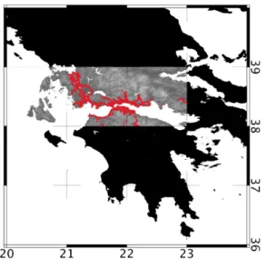
Fig. 1. Western Gulf of Corinth with the location of the three TanDEM-X tiles and, in red, the 148 kinematic GNSS surveys.
capability of monitoring and interpreting the changes mentioned above. In the case of large deformations, e.g., produced by earthquakes, changes might be detected between high-resolution DEMs and used jointly with InSAR. High-resolution DEMs constitute information of major interest for the long-term study of this area over decades and centuries. They contribute to bridging short-term deformations captured by GNSS and InSAR with the long-term deformation and the resulting topography. They contribute also to an accurate evaluation of the erosion processes which is needed to interpret the landscape and its relation with the active faulting.
The TanDEM-X DEM [12], [13] studied here was calculated in 2017 by the German Space Agency (Deutsches Zentrum für Luft- und Raumfahrt, DLR) with a mosaic of TerraSAR-X images acquired between 2011-02-20 and 2014-09-09. It has a nominal resolution of 2.5 pixels per arc s, which corresponds to 9.756 m in the EW axis and 12.329 m in the SN axis. The DEM of the CRL area is composed of three tiles of 1 x 1 degree each, which means 9001× 9001 pixels. By convention, the centers of the pixels are located at round coordinates. Therefore, the pixel located at the north-east edge of our eastern tile has its center at 20°E 39°N and its north-east corner at 19.9999444°E– 39.0000556°N. The accuracy and precision of the TanDEM-X DEM have been studied in several environments, e.g., [14], [15], with GNSS control points used in some cases, e.g., [16], [17] but not with the density of our control network. Another way to assess the precision of the DEM is with LIDAR observations [18]. We remind that accuracy characterizes the closeness of the DEM or the GNSS coordinates to the real shape of the ground, while precision represents the internal closeness between DEM and GNSS measurements.
II. GNSSKINEMATICSURVEYS
From 2001 to 2019, 148 kinematic GNSS surveys suitable for this analysis were performed. Fig. 1 shows the location of the surveys and Table I provides details for each year.
TABLE I KINEMATICGNSS SURVEYS
“GNSS points” indicates the number of points used for the quality assessment. The total number of GNSS points is 885 252.
The data was processed with the Canadian Spatial Reference System Precise Point Positioning (CSRS-PPP) online software. We compared its solutions with those of two other online software, GIPSY-PPP, and IGN-PPP, and with our local calculations made with GIPSY 6.4. We found that it was the one giving the best repeatability of the traces and the lower number of outliers. Moreover, for observations made after mid-2011, it processes not only the GPS (global positioning system) data but also the data of the GLONASS constellation, which is valuable in the case of kinematic observations that are very sensitive to the loss of satellites in vegetated or urban areas. All coordinates are expressed in ITRF2014 [19] which is consistent at a few millimeters level with the coordinates used for the TanDEM-X data in the datum WGS84-G1150.
We extract from our CSRS-PPP solutions the most precise epochs estimated by the calculation. Indeed, a compromise is needed to keep enough points and sample all areas including the urban and forest areas crossed during the surveys. We thus keep the epochs with at least six satellites, speed of the car above 2 m/s, uncertainties of the coordinates (as estimated by CSRS-PPP) below 0.1 m in horizontal and 0.2 m in vertical. We also eliminate the solutions with scatter DEM-GNSS larger than four meters as, during an initial analysis, we observed that the population of those outliers was below 1% of the total. For those outliers, we could not find any anomaly in the GNSS data so we believe that they are almost entirely due to anomalies in the DEM. Finally, our set of GNSS coordinates comprises 885 252 epochs, which represents a total course of∼7500 km if we assume an average speed of 30 km/h during the surveys.
A. Calibrating the Accuracy of the GNSS Surveys
As we cannot just rely on the theoretical uncertainties given by our kinematic GNSS software, some GNSS surveys were tailored specifically for assessing the accuracy of the data
Fig. 2. Kinematic GNSS survey performed on 2016-09-25 with three antennas operated on a vehicle (see video at https://youtu.be/1NDTSt0GZRI).
Fig. 3. In red, the survey of Sep. 25, 2016, and in the green box, the calibration area where multiple passes were acquired.
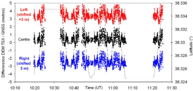
Fig. 4. Left: map of the road profile with GNSS elevation in color (meters above ellipsoid); right: latitude of the car as a function of time. Black box in the left graph shows the location of Fig. 6 and gray box the location of Fig. 8.
processing, using part of the experimental protocols validated in previous works [20]–[22]. On September 25, 2016, three receivers were operated on the same car as shown in Fig. 2, on a calibration trail observed periodically. The configuration with three antennas allows examining at the same time the repeatabil-ity along the repeated path and the fluctuations of the distances and relative heights between the antennas. The latter provides an evaluation of the GNSS data processing independent, at the first order, of the path of each antenna.
Fig. 5. Baseline of the three pairs of antennas as a function of time. The solid curve indicated the latitude of the vehicle (right vertical scale of the graph).
TABLE II
RELATIVELOCATION OF THEANTENNAS
Fig. 6. Elevation of the repeated passes in a 100-m section of the road (the location is shown in the small black box in Fig. 4).
Fig. 3 shows the location of the September 25, 2016 survey with, in red, the area for which the results are presented. The vehicle traveled five times from south to north and five times from north to south as shown in Fig. 4 (right), thus the road was sampled 27 times. We project along the latitude because the profile is predominantly north–south with no overlaps. Fig. 5 shows the evolution of the calculated distance between antenna pairs.
If the CSRS-PPP processing was perfect, the distances should not change while we observe fluctuations within 0.1 m peak-to-peak, with standard deviations listed in Table II. The jumps ob-served when the car reverses its route may be due to uncorrected clock biases in the modeling of the phase of the GNSS signals. Fig. 6 shows the elevation of the profiles in a 100-m section of the road. All are contained in an envelope of less than 0.2 m. From the analysis of this GNSS survey, we conclude that, in the case of a relatively open road like the one sampled on 2016-09-25, we can, with our method and the performance of the CSRS-PPP calculation, retrieve an accurate elevation of the road with a precision better than 0.1 m. This value is well below the scatters between the GNSS and the DEM as we will see in the next section. Thus, we can consider that our 885 252 GNSS
Fig. 7. Resampling at 1-m resolution a kinematic GNSS profile.
points constitute a nearly perfect ground truth for the assessment of the DEM, at least along the roads and trails of the area (that are indeed specific features in the imagery).
B. Generating GNSS Profiles in Steps of 1 m
In a survey along a trail like the one of September 25, 2016, the speed of the car does not exceed∼25 km/h, i.e., one point every∼7 m, while on asphalted roads the distance traveled in 1 s can reach 30 m. High speed usually means large open roads, hence good GNSS signal, and relatively flat and smooth surface, thus the DEM is expected to be very reliable. On the contrary, low speeds often correspond to narrow paths, with GNSS signal possibly of lower quality due to nearby vegetation and other masks, and the DEM not able to mimic the uneven topography below its native resolution.
Because of the accuracy of the GNSS and the smoothness of the GNSS trajectories, we found it possible to oversample our surveys in all places where they are continuous, and thus estimate one horizontal and vertical road coordinates every 1 m. Fig. 7 shows how the resampling was performed with a method that fits smoothly the curves.
The 1-m resampling gives more weight to the areas where we believe both the DEM and GNSS dataset are more reliable. This is the case in particular along the main roads where the vehicle is moving relatively fast with a three-dimensional (3-D) trajectory very smooth. It leads to an increase of one order of magnitude of our dataset from 885 252 to∼10.8 million points. Along most of the observed roads those points sample, pixel by pixel, the 1-m resampled TanDEM-X DEM, except in some rare forest and urban areas where GNSS data is missing because of the masks. With this oversampling and the redundancy of the surveys, most of the homologous pixels located on the surveyed roads contain several observations.
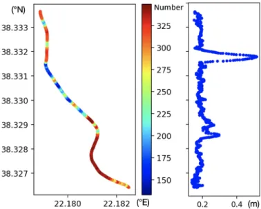
In the case of our calibration trail of Fig. 4, observed many times from 2001 to 2019, the total number of GNSS elevations ranges between 135 and 350 data points every 1 m along the path as shown in Fig. 8 (left). The standard deviation increases to∼0.2 m, which is twice that of the single survey of September 25, 2016, because of the different experimental conditions. Fig. 8 (right) also shows a local peak of 0.5 m in a place where the road was reworked for the installation of wind engines nearby (visible in the video).3 We consider that this value of 0.2 m is a good
estimate of the accuracy of the vertical coordinates of our GNSS
3[Online]. Available: https://youtu.be/1NDTSt0GZRI
Fig. 8. Left: number of resampled points every 1 m along a section of the path of Sep. 25, 2016 (the location is shown in the inset of Fig. 4 left), using all those of the 148 surveys performed in the same area; right: standard deviation of the road elevation (m) estimated every 1 m along the calibration road.
points. As we will see below, this accuracy is five times better than that of the TamDEM-X DEM and therefore appropriate for the assessment of the DEM’s accuracy.
III. VERTICALACCURACY OF THETANDEM-X DEM We now compare the TanDEM-X DEM with the elevation of the GNSS points using strategies already used in previous works [21], [22], and other guidelines for DEM assessment [23], [24]. We use two different approaches, the first one is using the whole GNSS data set as a global entity and the second one is based on a preliminary survey-per-survey analysis.
A. Resampling of the DEM
We first resample the DEM at a higher resolution. Indeed, its native resolution is too coarse to take into account precisely enough the local slopes and the exact location of the GPS points within the pixels. Resampling the DEM by a factor of 10 leads to pixels of size∼1 m, which allows efficient comparison of the DEM and GNSS, as this size is smaller than the width of the sampled road even the smallest ones.
We tested a bilinear interpolation and a cubic interpolation (see validation in Section IV-C) and hereafter we use the second one because, as we will see later, it leads to lower scatters between the DEM and the GNSS. The resampling is performed with the GDAL software package, using the GDAL VRT (virtual data set) routine. The instruction to make the resampling is “gdalbuildvrt -tr 0.000011111 0.000011111 -r cubic dem.vrt
∗tif” with dem.vrt name of the virtual DEM and ∗tif our three
TanDEM-X tiles in their original tif format. The resampled virtual DEM is a matrix of 270 010 × 90 010 pixels, with a size of 0.00001111° (25 pixels per arc s), thus 0.9756 m in the EW axis and 1.2329 m in the SN axis.
Fig. 9. Histogram of the difference TanDEM-X minus GNSS. In red, the mean value, and in black the quartiles. The median is at 0.376 m.
Fig. 10. Vertical shift TanDEM-X–GNSS of the whole set of 885 252 points.
Fig. 11. Areal distribution of the scatters between TanDEM-X and GNSS elevations for the whole set of 885 252 GNSS points.
B. Vertical Shift With Respect to All the GNSS Points
Fig. 9 shows the histogram of the difference DEM-GNSS for the whole set of 885 252 points. Using the mean as the metric, the DEM is shifted upward by 0.466 m with respect to the GNSS. The histogram is not perfectly symmetric and the median is 0.376 m thus 0.09 m below the mean.
Fig. 10 shows the difference DEM-GNSS of the whole dataset plotted as a function of the elevation. The colors show the density of points. Most points are located at low elevation, with a gentle density decrease while going up. All elevations are sampled up to 1750 m which is close to the∼2200 m top elevation of the area. Fig. 11 shows that the areal distribution of the scatters is relatively homogeneous. To the northwest, some red sections fit with the location of a highway built after the production of the DEM. The mean standard deviation of the 885 252 scatters DEM-GNSS is 1.124 m. This shows that, after correction of the shift, the DEM has, a 1-m precision in the CRL area, at least along the surveyed roads and trails.
Fig. 12. For the 148 surveys, mean scatter in longitude, latitude, and elevation between the TanDEM-X DEM and GNSS. The left and right calibration surveys of Sep. 25, 2016 are shown with the red and blue dots. For the elevation, in red the best fitting second-order polynomial.
C. Vertical Shift From a Survey Per Survey Analysis
Since we have a large number of surveys, we can also assess independently the accuracy and precision of each one, and then combine the evaluations. This allows detecting and handling, separately for each survey, possible errors of antenna height measurement or other biases of any type associated with the specific receiver and antenna used. Those biases are likely to induce spatially correlated shifts within the affected surveys.
For each survey, we calculate the mean shift between the DEM and the GNSS points, and its root mean square (rms) scatter. Fig. 12 shows those values plotted as a function of longitude, latitude, and elevation. The rms scatters are plotted as uncertainties bars on the Y-axis. With this method, looking at the mean of all means, the average scatter DEM-GNSS is now 0.495± 0.026 m, close to the 0.466 m found previously. The uncertainty is estimated by dividing the mean of the 148 rms scatters (0.315 m) by the square root of the number of observations (148), assuming a Gaussian distribution of the 148 single rms scatters. The fact that the value of 0.315 m is larger than the 0.2 m mean accuracy of our GNSS coordinates (as determined in Section II-B), suggests the possible existence of spatial heterogeneities of the anomalies of the DEM with respect to the GNSS.
Fig. 12 shows that the DEM is shifted homogeneously in the entire area without tilts. It shows also no dependence at the first order of the shift with the elevation, yet when we fit the data with a second-order polynomial, we see a slight dependence.
Fig. 13. Difference TanDEM-X–GNSS as a function of time for the three antennas during the survey of Sept. 25, 2016.
Fig. 14. Difference TanDEM-X–GNSS as a function of latitude.
D. Precision of the Single September 25, 2016 Survey
The survey of September 25, 2016 (see Section II-A) allows us to analyze locally the vertical shift DEM-GNSS in an area with highly redundant data. Fig. 13 shows the vertical offset (for the three antennas all together), which is 0.503 m, thus very close to the overall offset found previously.
The rms scatter of the difference DEM-GNSS at each sample point is 0.493 m, thus in this calibration area, the vertical precision of the DEM (as assessed by the GNSS data) is∼0.5 m, two times less than its 1.086 m global precision estimated in Section II-B. The scatters range between −0.5 m and 1.5 m as shown in Fig. 14, with fluctuations in various spatial wavelengths.
E. Urban and Forest Areas
The roads traveled during the 148 surveys cross different types of land cover including urban and forest areas. By extracting 9254 and 25 266 points belonging, respectively, to urban and forest areas (Fig. 15), we find that the DEM overestimates on average the elevation by 1.12 m in the former and 0.95 m in the latter, thus an extra overestimation of∼0.53 m with respect to the overall shift of the DEM. The detailed analysis of those areas is beyond the objectives of this article.
IV. HORIZONTALACCURACY OF THEDEM
The mountainous CRL area is well adapted for evaluating the accuracy of the georegistration of the TanDEM-X DEM. Indeed, when a DEM shows a general slope, horizontal and vertical shifts are not independent: a downwards translation would mimic a shift in the downslope direction and vice versa.
Fig. 15. Urban (blue) and forest (green) areas within the kinematic GNSS data.
Fig. 16. Exploration of the 3-D space of TanDEM-X–GNSS deviationδ, for vertical shifts (applied to the DEM) ofγ = −0.2 m (left) and γ = −0.5 m (right).
Fig. 17. Cross-sections across the 3-D space of TanDEM-X–GNSS deviation
δ for a vertical shift (applied to the DEM) γ = −0.5 m and nine eastward shifts.
A. Global Analysis of the Whole Dataset
We offset the DEM in steps of 0.1 m in longitude, latitude, and elevation, and calculate at each step the rms scatter between DEM and GNSS elevations, hereafter calledδ. As an example, Fig. 16 shows the distribution ofδ as a function of the longi-tudinal and latilongi-tudinal offsets α and β, for two values of the vertical offsetγ of −0.2 m (left) and −0.5 m (right). The latter leads to lower deviations, which was expected as we know from Section II-B and II-C that the vertical shift is close to−0.5 m. Fig. 17 shows that, at the first order, δ evolves as a parabolic function of the variablesα, β, and γ, which can be written as follows:
Fig 18. Rms as a function of the horizontal shift of the DEM for the central antenna of the survey of Sep. 25, 2016. The scatters are minimized with a DEM shifted by 0.87 m toward the south and 0.14 m toward the west.
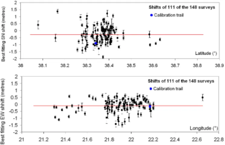
Fig. 19. Best fitting EW and SN shifts from the analysis of the single determi-nations of 111 among the 148 surveys. In blue, the point representing the shift of the calibration trail of Sep. 25, 2016 (see also Fig. 18).
A least-square fit gives the following values for the polyno-mial coefficients: A= 0.0242, B = 0.0189, C = 0.4349, D =
−0.0111, E = 0.0002, F = 0.4349, G = 1.2194, H = −0.0135,
I= −0.0285.
The rms scatterδ is minimal and is δ0 = 1.125 m for the following values of the variables:α0= −0.099 m, β0= −0.360 m,γ0= −0.467 m. Those values indicate by how much the DEM must be shifted in longitude, latitude, and elevation to give the best fit of the DEM to the GNSS ground truth.
B. 3-D Shift From a Survey Per Survey Analysis
Here, like in Section III-C, we first estimate the shift (now in 3-D) for every single survey. For each, we shift the DEM by
−2, −1, 1, and 2 m in longitude, and −2, −1, 1, and 2 m in
latitude, and calculate the mean shift and the rms scatter for the eight cases. Fig. 18 shows the example of the calibration survey of 2016-09-25 (central antenna).
By fitting the two sets of rms scatters with a second-order polynomial, we can estimate the longitudinal and latitudinal shifts that minimize the scatter. In the particular case, the best fit is obtained with a shift of−0.14 m in longitude and −0.87 m in latitude.
Only 111 of the 148 surveys give a distribution of rms scatters that can be fitted with a second-order polynomial. Fig. 19 shows the values of the best fitting longitudinal and latitudinal scatters for those surveys. They are plotted as a function of longitude
Fig. 20. Relation between horizontal and vertical shifts of the DEM.
Fig. 21. Difference of vertical shift when using the original 885 252 GNSS points or the 1-m resampled 10.8 millions points.
and latitude, respectively, which allows us to see that there is no lateral variation. The standard deviations are 0.476 m in longitude and 0.620 m in latitude. Those values are relatively large, but this is not surprising as the horizontal control of the DEM by using GNSS is necessarily less good than the vertical control, in a ratio that should be roughly proportional to the average slope in the sampled areas. The mean of the 111 shifts is−0.11 ± 0.13 m in longitude and −0.28 ± 0.18 m in latitude, which is consistent with what was found in the previous section. The uncertainties are the average scatters divided by the square root of the number of surveys.
Our analysis, using two different methods, shows that the lateral shift of the DEM is well below 1 m. It is remarkable that our GNSS dataset permitted us to make this assessment. Moreover, by using GNSS points on both sides of the gulf and outside of it, we ensured the presence of slopes in all azimuths in the dataset, which reduces the covariance between vertical and horizontal shifts.
Looking now at the best fitting vertical shifts of the DEM, associated with the best fitting rms scatters, Fig. 20 shows that their dependence as a function of longitude and latitude can be assessed precisely. For example, when the DEM is shifted northward (red curve), the vertical shift between the DEM and the GNSS becomes lower, which is understandable intuitively and is quantified here.
C. Using the GNSS Data Resampled at 1 m
We redo the analysis of Section IV-A with the resampled 10.8 million GNSS coordinates presented in Section II-B. This resampled dataset contains more additional points where the ve-hicles are moving fast, thus along the large roads and highways. The values of the best fitting shifts in longitude, latitude, and height becomeα = −0.024 m, β = −0.023 m, γ = −0.338 m. The rms scatter is now 1.150 m, very close to the previous one.
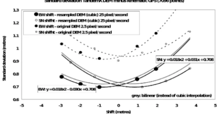
Fig. 22. Standard deviation of the scatter DEM-GNSS in the area of the Sep. 25, 2016 survey when using the original DEM and the resampled DEM with the two different interpolations procedures.
In horizontal, the DEM appears now to be perfectly accurate. In the vertical, there is a small (well below the value of the rms scatter) but significant difference of 0.13 m with the range of values ofγ found previously, and quite systematic in most of the surveys as shown in Fig. 21.
This difference is presumably an attenuated global effect of similar origin to the one that causes the overestimated shift of 0.53 m of the DEM in the urban and forest areas discussed in Section III-E. Outside forest and urban areas, the small roads and trails represent a significant part of our surveys. There, the TanDEM-X DEM would correspond on average to objects slightly higher (one to two decimeters) than the surface of roads. A more detailed analysis is beyond the objectives of this article, but this difference shows that the location of the sampled GNSS points is not neutral in the evaluation of a DEM with the quality of TanDEM-X.
D. Importance of the Cubic DEM Interpolation
Fig. 22 illustrates how the standard deviations vary, in the case of our calibration area of September 25, 2016, when using the DEM not resampled and the DEM resampled with both interpolations. The cubic resampling leads to the lowest stan-dard deviations, reaching the lowest value of 0.695 m (for that particular surveyed area), while it is 0.73 m for the bilinear case and 0.91 m when no resampling is applied.
V. CONCLUSION
Using a dense and accurate set of GNSS coordinates produced by 148 kinematic GNSS surveys performed from 2001 to 2019 in the western Gulf of Corinth, covering a total distance of∼25 000 km, we establish that 1) the average vertical accuracy of our GNSS data is∼0.2 m, 2) the TanDEM-X DEM is shifted with respect to the GNSS ground true by −0.10 ± 0.10 m toward the east, and−0.36 ± 0.10 m toward the north, −0.47 ± 0.03 m toward up. Those values are 20 times below the nominal resolution of the DEM.
We observe no lateral tilt of the DEM over the entire area and no or minor dependence of the vertical DEM offset as a function of the elevation.
After shifting the DEM to its right vertical location, the rms deviation between the DEM and the GNSS ground truth is 1.125 m. This average scatter is below the nominal expected precision of the TanDEM-X DEM [13] and below the values found in some publications where GNSS is used to assess its precision, e.g., [23]. The scatter DEM-GNSS has components in a wide range of spatial wavelengths.
We verified that resampling the original set of 885 252 GNSS coordinates in profiles of 1-m steps can be done safely. This resampling allows to create an almost complete coverage of the roads of the area at this 1-m resolution with an accuracy of 0.2 m for any single point, thus an expected accuracy of 0.02 m for portions of road of 100 m length assuming a Gaussian distribution of the errors.
We could assess the horizontal location of the TanDEM-X DEM. This is valuable for the optimization of the registration of the metric size ortho-images that go along with the DEM.
The GNSS surveys are made along roads and trails only, so they cannot tell directly what are the accuracy and the precision outside of those features. However, when plotting sections per-pendicular to the roads we could not see in the DEM a specific signature of the roads, except for some highways newly built. Therefore, we believe that our evaluation of the DEM can be widened to most of the entire area, except perhaps high slopes, urban, and forest areas where the nominal resolution does not permit to get everywhere to the ground level. In areas of high relief, like river banks, limitations of the TanDEM-X DEM are indeed reported in the literature, e.g., [26].
The accuracy and precision of the TanDEM-X DEM is ap-proximately five times better than that of the EU-DEM calibrated on another region of Greece [27]. This makes the TanDEM-X DEM a valuable tool for monitoring the topographic changes occurring in an active tectonic area like the CRL. In the case of a large earthquake, which is occurring typically every few decades [28], the seismic rupture can reach the surface and shift it from a few centimeters to a few decimeters over distances of several hundred meters to a few kilometers. In such a case, DEM having the quality of the TanDEM-X DEM can contribute to quantifying local vertical ground deformations, provided that two DEMs are available, one before and one after the event. In the last 10 years, there was not such a large event but there were active landslides and active erosion phenomena along the rivers and the shores of the gulf. Those changes might already be detectable by comparing two TanDEM-X DEM produced at two different epochs separated by a few years.
Our study leaves open questions, e.g., is the metric precision of the DEM found along roads still valid in the rest of the DEM? Would the comparison of two TanDEM-X DEM (or DEM with equivalent precision) allows us to confirm the scatters found in some sections of newly built highroads?
SUPPORTINGINFORMATION
1) PDF containing metadata for the 148 GNSS surveys and description of the format of the CSV files.
2) CSV files with the three-dimensional coordinates of the 885 252 selected GNSS points.
ACKNOWLEDGMENT
The authors would like to thank all the colleagues and students who were involved in the 148 kinematic surveys carried out from 2001 to 2019, in particular Ferdaous Chaabane, Rana Charara, Michalis Delagas, Anne Deschamps, Emilie Klein, Kamel Lam-mali, Marine Roger, Nikos Roukounakis, Luca Terray, Maurin Vidal, and Christophe Vigny. Most of the GNSS receivers used were provided by the “GPSMOB” pool of GNSS receivers of the French CNRS. They would like to thank the Canadian Geodetic Survey of Natural Resources for making available on-line the CSRS-PPP service that they used to process the kinematic GNSS data. For some figures, they used the Generic Mapping Tool [29]. They would like to thank the German Aerospace Center (DLR) for making available the TanDEM-X DEM in the framework of the science project DEM_CALVAL2013 “Corinth Rift Laboratory TanDEM-X DEM and kinematic GNSS array.” The authors would also like to thank the three reviewers for their corrections and comments that improved the manuscript.
REFERENCES
[1] F. H. Cornet, P. Bernard, and I. Moretti, “The corinth rift laboratory,” C.R.
Geosci., vol. 336, pp. 235–241, 2004.
[2] P. Briole et al., “Active deformation of the corinth rift, Greece: Results from repeated global positioning system surveys between 1990 and 1995,”
J. Geophys. Res.-Solid Earth, vol. 105, no. B11, pp. 25605–25625, 2000.
[3] P. Elias and P. Briole, “Ground deformations in the corinth rift, Greece, investigated through the means of SAR multitemporal interferometry,”
Geochem. Geophys. Geosyst., vol. 19, no. 12, pp. 4836–4857, 2018.
[4] S. Neokosmidis, P. Elias, I. Parcharidis, and P. Briole, “Deformation estimation of an earth dam and its relation with local earthquakes, by exploiting multitemporal synthetic aperture radar interferometry: Mornos dam case (Central Greece),” J. Appl. Remote Sens., vol. 10, no. 2, 2016, Art. no. 026010.
[5] A. Papadopoulos, I. Parcharidis, P. Elias, and P. Briole, “Spatio-temporal evolution of the deformation around the Rio-Patras fault (Greece) observed by synthetic aperture radar interferometry from 1993 to 2017,” Int. J.
Remote Sens., vol. 40, no. 16, pp. 6365–6382, 2019.
[6] I. Parcharidis, M. Foumelis, G. Benekos, P. Kourkouli, C. Stamatopoulos, and S. Stramondo, “Time series synthetic aperture radar interferometry over the multispan cable-stayed Rio-Antirio bridge (central Greece): Achievements and constraints,” J. Appl. Remote Sens., vol. 9, no. 1, 2015, Art. no. 096082.
[7] T. Lebourg, S. E. Bedoui, and M. Hernandez, “Control of slope deforma-tions in high seismic area: Results from the gulf of Corinth observatory site (Greece),” Eng. Geol., vol. 108, no. 3–4, pp. 295–303, 2009. [8] N. Palyvos, F. Lemeille, D. Sorel, D. Pantosti, and K. Pavlopoulos,
“Geo-morphic and biological indicators of paleoseismicity and holocene uplift rate at a coastal normal fault footwall (western Corinth Gulf, Greece),”
Geomorphology, vol. 96, no. 1–2, pp. 16–38, 2008.
[9] P. M. De Martini, D. Pantosti, N. Palyvos, F. Lemeille, L. McNeill, and R. Collier, “Slip rates of the Aigion and Eliki faults from uplifted Marine terraces, Corinth gulf, Greece,” C.R. Geosci., vol. 336, no. 4–5, pp. 325–334, 2004.
[10] A. Ganas, S. Pavlides, and V. Karastathis, “DEM-based morphometry of range-front escarpments in Attica, central Greece, and its relation to fault slip rates,” Geomorphology, vol. 65, pp. 301–319, 2005.
[11] C. Tsimi, A. Ganas, N. Soulakellis, P. Kairis, and S. Valmis, “Morpho-tectonics of the psathopyrgos active fault, western Corinth rift, central Greece,” Bull. Geol. Soc. Greece, vol. 40, no. 1, pp. 500–511, 2007. [12] G. Krieger et al., “TanDEM-X: A satellite formation for high-resolution
SAR interferometry,” IEEE Trans. Geosci. Remote Sens., vol. 45, no. 11, pp. 3317–3341, Nov. 2007.
[13] P. Rizzoli et al., “Generation and performance assessment of the global TanDEM-X digital elevation model,” ISPRS J. Photogramm. Remote Sens., vol. 132, pp. 119–139, 2017.
[14] P. Rizzoli, B. Bräutigam, T. Kraus, M. Martone, and G. Krieger, “Relative height error analysis of TanDEM-X elevation data,” ISPRS J. Photogramm.
Remote Sens., vol. 73, pp. 30–38, 2012.
[15] K. Gdulová, J. Marešová, and V. Moudrý, “Accuracy assessment of the global TanDEM-X digital elevation model in a mountain environment,”
Remote Sens. Environ., vol. 241, 2020, Art. no. 111724.
[16] J. Baade and C. Schmullius, “TanDEM-X IDEM precision and accuracy assessment based on a large assembly of differential GNSS measurements in Kruger national park, South Africa,” ISPRS J. Photogramm. Remote
Sens., vol. 119, pp. 496–508, 2016.
[17] B. Wessel, M. Huber, C. Wohlfart, U. Marschalk, D. Kosmann, and A. Roth, “Accuracy assessment of the global TanDEM-X digital elevation model with GPS data,” ISPRS J. Photogramm. Remote Sens., vol. 139, pp. 171–182, 2018.
[18] K. Zhang, D. Gann, M. Ross, H. Biswas, Y. Li, and J. Rhome, “Comparison of TanDEM-X DEM with LiDAR data for accuracy assessment in a coastal urban area,” Remote Sens., vol. 11, no. 7, 2019, Art. no. 876.
[19] Z. Altamimi, P. Rebischung, L. Metivier, and X. Collilieux, “ITRF2014: A new release of the international terrestrial reference frame modeling non linear station motions,” J. Geophys. Res.-Solid Earth, vol. 121, no. 8, pp. 6109–6131, 2016.
[20] C. Deplus and P. Briole, “Measurement of profiles using kinematic GPS. Results of an experiment made in Crete in October 1996,” (in French) Zenodo, 1997.
[21] P. Baldi, S. Bonvalot, P. Briole, and M. Marsella, “Digital photogrammetry and kinematic GPS applied to the monitoring of Vulcano island, Aeolian arc, Italy,” Geophys. J. Int., vol. 142, no. 3, pp. 801–811, 2000. [22] A. Mouratidis, P. Briole, and K. Katsambalos, “SRTM 3 arc second DEM
(versions 1, 2, 3, 4) validation by means of extensive kinematic GPS measurements: A case study from N. Greece,” Int. J. Remote Sens., vol. 31, no. 23, pp. 6205–6222, 2010.
[23] J. Höhle and M. Höhle, “Accuracy assessment of digital elevation models by means of robust statistical methods,” ISPRS J. Photogramm. Remote
Sens., vol. 64, pp. 398–406, 2009.
[24] J. L. Mesa-Mingorance and F. J. Ariza-López, “Accuracy assessment of digital elevation models (DEMs): A critical review of practices of the past three decades,” Remote Sens., vol. 12, 2020, Art. no. 263.
[25] L. Guan, H. Pan, S. Zou, J. Hu, X. Zhu, and P. Zhou, “The impact of horizontal errors on the accuracy of freely available digital elevation models (DEMs),” Int. J. Remote Sens., vol. 41, no. 19, pp. 7383–7399, 2020.
[26] S. J. Boulton and M. Stokes, “Which DEM is best for analyzing flu-vial landscape development in mountainous terrains?,” Geomorphology, vol. 310, pp. 168–187, 2018.
[27] A. Mouratidis and D. Ampatzidis, “European digital elevation model validation against extensive global navigation satellite systems data and comparison with SRTM DEM and ASTER GDEM in central macedonia (Greece),” ISPRS Int. J. Geo-Inf., vol. 8, no. 3, 2019, Art. no. 108. [28] P. Albini, A. Rovida, O. Scotti, and H. Lyon-Caen, “Large eighteenth–
nineteenth century earthquakes in western Gulf of Corinth with reap-praised size and location,” Bull. Seismol. Soc. Amer., vol. 107, no. 2, pp. 1663–1687, 2017.
[29] P. Wessel and W. Smith, “New improved version of the generic map-ping tool released,” Eos, Trans. Amer. Geophys. Union, vol. 79, 1998, Art. no. 579.
Pierre Briole received the M.Sc. degree in electronics, electrical engineering,
and automatics from the University Paris Sud, Orsay, France, in 1982, the agréga-tion of physics, opagréga-tion applied physics, in 1983, the Ph.D. degree in geophysics from the University Paris VI, Paris, France, in 1990, and the habilitation à Diriger des Recherche from the University Paris VII, Paris, France, in 2000.
After spending two years on Mt. Etna, Italy with the International Institute of Volcanology, he joined the Institut de Physique du Globe in Paris where he developed applications of GPS and SAR interferometry to volcanoes and seismic faults monitoring and the geophysical modeling of ground deformations. In 2007, he joined the Laboratory of Geology, Ecole Normale Supérieure.
Dr. Briole is a member of the French Bureau des Longitudes and the current President of the Comité National Français de Géodésie et Géophysique.
Simon Bufféral was born in Clermont-Ferrand, France, in 1995. He received
the M.Sc. degree from the École Normale Supérieure, University Paris VI, Paris, France, in 2015, and the agrégation in sciences of earth, life and universe, in 2019.
During the last years, he participated in various GNSS campaigns aiming at monitoring active volcanoes, faults, and crustal deformation in Greece and Italy, and in geological surveys in the Philippines, New Caledonia, and Greece. His research interests include geodynamics and structural geology.
Dimitar Dimitrov received the M.Sc. degree in geodesy from the Insitute of
Architecture, Civil Engineering and Geodesy, Sofia, Bulgaria, and the D.Sc. and Ph.D. degrees in geodesy from the National Scientific Commission, Sofia, Bulgaria, in 1995 and 2009, respectively.
He is currently with the Department of Geodesy, National Institute of Geo-physics, Geodesy and Geography, Bulgarian Academy of Sciences, Sofia, Bul-garia. His research interests include ENS, Paris, France—include measurement and modeling of GPS/GNSS data, and their application in the study of seismic deformations.
Panagiotis Elias received the M.Sc. degree in signal processing for
telecom-munications and multimedia from the University of Athens, Athens, Greece, in 2007, and the Ph.D. degree in geosciences within the framework of cotutelle agreement from the École Normale Supérieure, Paris, France and the University of Patras, Patras, Greece, focused in space geodesy, in 2013.
He joined the Institute for Astronomy, Astrophysics, Space Applications and Remote Sensing of the National Observatory of Athens, Athens, Greece, in 2005. His research interests include satellite geodesy and modeling for geophysical applications.
Dr. Elias is a member of the Remote Sensing and Space Applications Exec-utive Committee of the Hellenic Geological Society.
Cyril Journeau received the M.Sc. degree in geophysics from the University
Paris Diderot, Paris, France, in 2019. He is currently working toward the Ph.D. degree at the Institut des Sciences de la Terre (University Grenoble Alpes)—in cooperation with the Volcanological Observatory of Piton de la Fournaise—on the analysis of volcanic processes from measurements of seismic and geodetic networks at Piton de la Fournaise (La Réunion Island, France) and at the Klyuchevskoy Volcanic Group (Kamchatka, Russia).
During his studies, he completed internships with the Laboratory of Geology of Ecole Normale Supérieure, Paris, France, at GNS Science in New Zealand, and with the Institut de Physique du Globe, Paris, France.
Antonio Avallone received the M.Sc. degree in geological sciences with
spe-cialization in geophysics from the University of Naples “Federico II,” Naples, Italy, in 1998, and the Ph.D. degree from the Institut de Physique du Globe of Paris, Paris, France, in 2003.
Since 2004, he has been a Researcher with the Istituto Nazionale di Geofisica e Vulcanologia. He is working on the collection and analysis of GPS data to study the evolution of the deformation at different spatial and temporal scales, in particular in the active tectonic domain of the Mediterranean region. He is deeply involved in the development of a permanent real-time GNSS network. His research interests include use and analysis of high-rate GNSS data for better understanding the processes during and after an earthquake and the real-time processing for early warning applications.
Konstantinos Kamberos received the Graduate degree in geodesy from the
School of Rural and Surveying Engineering, National and Technical University of Athens, Athens, Greece, in 2000.
From 1993 to 1998, he participated in several GPS missions with the Gulf of Corinth and in two post-earthquake missions (Aegio and Kozani), in 1995. In 1993 and 1995, he processed GPS measurements at the IPGP Seismological Laboratory for Analyzing the Deformations of Gulf of Corinth. Until 2007, he worked in the construction of public works (Patras bypass highway, Tithorea-Leianokladi railway, and Corinth-Kiato railway). Since 2007, he has been with the ERGOSE SA (public company for the management of the construction works of the new railway line of Greece), project manager in the Peloponnese area.
Michel Capderou received the Ph.D. degree in atomic physics, on the topic of
metastability of neutral argon, from the University of Toulouse III, Toulouse, France, in 1972.
From 1974 to 1989, he was a Research Fellow with the University of Alger, Alger Ctre, Algeria. In 1989, he joined the University Pierre et Marie Curie (now Sorbonne University), Paris, France, where he was teaching until 2015. He is doing research with the Laboratoire de météorologie dynamique (LMD), Sorbonne University, and École Polytechnique, France. He worked on the design, modeling, and observation of the satellite orbits. He wrote a Handbook of
Satellite Orbits: From Kepler to GPS (Springer, 2014). He has authored an
orbitography and sampling software called Ixion, designed for the satellites of the Earth, Mars, and other celestial bodies. His research interests include Earth’s radiation balance, the preparation of space missions for the study of the Earth and Martian atmosphere, and the orbital strategy.
Alexandre Nercessian received the Ph.D. degree in geophysics from the
Uni-versity Paris VI, Paris, France, in 1980.
From 1973 to 1980, he was translating articles and scientific and technical books. He joined the Institut Fançais du Pétrole in 1982, and then the Institut de Physique du Globe de Paris, in 1983, where he got a full time position of Observatory Assistant, in 1985. His research interests include seismology, signal processing, electronics, with application to the monitoring of seismic zones and volcanoes. He has been deeply involved for more than three decades in the routine monitoring of the French volcanoes. He also took part in more than 15 marine geophysics cruises in the Pacific, Atlantic, Indian oceans, and the Mediterranean sea.