A Contractor Based on Convex Interval Taylor

Our method uses the geometrical properties of the vector field given by the ODE and a state space discretization to compute an enclosure of the trajectories set that verifies the

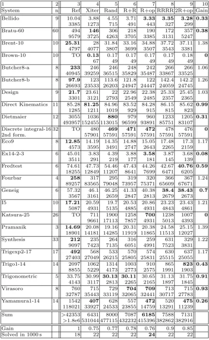
A common question when optimization algorithms are proposed is the com- putational complexity (also called computational cost or effort, CE) [9]. Usu- ally, the CE of swarm methods

It is clear that the location of the tales in the Cent Nouvelles nouvelles therefore perform important narrative work in the collection, and in particular that

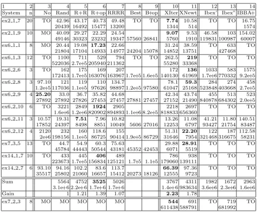
This real example is taken into account in this paper because it allows to show perfectly the great efficiency of (simple) propagation techniques inside classical

A common question when optimization algorithms are proposed is the com- putational complexity (also called computational cost or effort, CE) [9]. Usu- ally, the CE of swarm methods

Our method uses the geometrical properties of the vector field given by the ODE and a state space discretization to compute an enclosure of the trajectories set that verifies the

Unlike the response event, the interrupt event is not constrained by timing properties TP and does not block if there is no active interval instance to interrupt.. The interrupt

We propose a (double) penalization approach for solving the bilevel optimization problem, with a different treatment of the two constraints: a basic penalization of the easy