HAL Id: hal-01847274
https://hal.archives-ouvertes.fr/hal-01847274
Submitted on 7 Aug 2018
HAL is a multi-disciplinary open access
archive for the deposit and dissemination of
sci-entific research documents, whether they are
pub-lished or not. The documents may come from
teaching and research institutions in France or
abroad, or from public or private research centers.
L’archive ouverte pluridisciplinaire HAL, est
destinée au dépôt et à la diffusion de documents
scientifiques de niveau recherche, publiés ou non,
émanant des établissements d’enseignement et de
recherche français ou étrangers, des laboratoires
publics ou privés.
Subcarriers Number
Vincent Savaux, Yves Louët
To cite this version:
Vincent Savaux, Yves Louët. PAPR Analysis as a Ratio of Two Random Variables: Application to
Mul-ticarrier Systems with Low Subcarriers Number. IEEE Transactions on Communications, Institute of
Electrical and Electronics Engineers, 2018, 66 (11), pp.5732-5739. �10.1109/TCOMM.2018.2857460�.
�hal-01847274�
PAPR Analysis as a Ratio of Two Random
Variables: Application to Multicarrier Systems with
Low Subcarriers Number
Vincent Savaux and Yves Lou¨et
Abstract—The distribution of the peak to average power ratio
(PAPR) of multicarrier systems is studied in the context of signals featuring low subcarriers number. Considering the mean power of the signal as a random variable, a general cumulative distribution function of the PAPR is suggested. We show that the new formulation is valid not only for low subcarriers number, but also for larger subcarriers number. Thus, an asymptotic analysis using a large subcarriers number proves a perfect concordance between the suggested approach and the state-of-the-art derivations only valid for large subcarriers number. All the theoretical developments are supported through simulations, and we discuss the case of oversampled signals as well.
Index Terms—PAPR, CCDF, Multicarrier, OFDM.
I. INTRODUCTION
Multicarrier signals are well known to be prone to high power fluctuations due to the inherent summation of indepen-dent information carried on different tones. The most common way to quantify these power fluctuations is to define a metric taking into account its maximum value relatively to its mean. This gave birth to the peak factor definition namely the peak to average power ratio (PAPR) parameter highly discussed for decades especially in the context of multicarrier systems, such as orthogonal frequency division multiplexing (OFDM) (see [1] and references therein). PAPR is defined as the ratio of the maximum power and the mean power of a signal. An accurate PAPR derivation of multicarrier signal may be difficult given the initial statistic of the signal to be considered. A straightforward way to circumvent this issue is to directly upper bound the PAPR value regardless of any statistical hypothesis. As a result, a PAPR upper bound is found to be equal to N.f (M ), N being the useful subcarriers number of the OFDM systems and f (M ) a real value depending on the digital modulation constellation size M (it is easily shown that f (M ) equals 3MM +1−1). However this upper bound appears to be very far from reality and almost never reached due to the random behavior of the signal. As a consequence, the only way to provide a thorough PAPR model is to derive its distribution function or similarly its complementary cumulative distribution function (CCDF) viewing PAPR as a random variable due to the random character of the signal itself.
Manuscript submitted in March 2018
Vincent Savaux is with IRT b<>com, Rennes, France (e-mails: [email protected], Phone: +33 256 35 82 16.)
Yves Lou¨et is with CentraleSup´elec and IETR, Rennes, FR (e-mail: [email protected])
Considering a large subcarriers number N , a conventional analysis assumes that each time sample of the OFDM signal follows a complex Gaussian distribution. The overall signal can then be modeled as a random vector of N independent Gaussian samples. This has been first considered in [2], [3] where the CCDF of the PAPR is given in a very simple form and remains one of the most popular derivation. But the latter derivation ((2) in the paper) remains only valid for an oversampling factor equal to 1, which makes the formula inaccurate for oversampled signals simulating continuous phe-nomenons. The reason is that oversampling leads to correlated samples. Still in [2], [3], the authors extended their work to provide an approximation of the PAPR CCDF valid for large oversampling factors, but this approximation is empirical and yields some discrepancies with simulations for low subcarriers number (N < 128).
To extend [2], authors suggested more thorough derivations valid for lower oversampling values (4 or 8) [4]–[7] and different subcarriers numbers. These works are based either on the level crossing rate analysis of the peak distribution (since the envelop of the OFDM signal can be approximated as a Gaussian process), or theoretical links between peaks of sampled and continuous signals, called extreme value theory. However, these suggested expressions of PAPR CCDF are close to the simulation results only for N ≥ 64.
Nevertheless the recent interest in OFDM systems with low subcarriers number (e.g. narrowband internet of things (NB-IoT) signal with 12 subcarriers [8]) should push us to revisit the aforementioned PAPR derivations. The reason lies in the PAPR denominator expression: it could not be approximated as the signal power expectation as previously, since the ergodic condition is not valid anymore. Even though the central limit theorem remains valid (down to 10 carriers [9]), the denominator itself has to be reconsidered as a random variable and no more as a constant value (the mean power).
Thus, the main contributions of this paper are summarized as follows.
1) We derive a general PAPR cumulative function valid for large and low subcarriers numbers, down to 12 subcar-riers. Our results are supported by original theoretical developments. The main point is that the denominator of PAPR CCDF is viewed as a random variable. 2) We show that an asymptotic analysis for large N leads
to existing results [2], [3], which confirms the validity of our approach. Moreover, the first and second order moments of PAPR are derived from our suggested
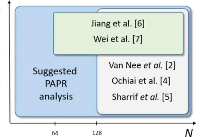
Fig. 1. Overview of the suggested PAPR analysis compared with state-of-the-art, according to subcarriers N and oversampling factor L.
CCDF, and perfectly match those found in the state of the art [4].
In addition, simulations results validate the theoretical devel-opments, which shows the interest to reconsider PAPR expres-sion for low subcarriers number. Furthermore, we discuss the extension of PAPR CCDF for low N value and large oversam-pling rate. Fig.1 positions the suggested work according to the number of subcarriers N and the oversampling factor L. Such as highlighted in Fig. 1, the suggested CCDF is relevant for low N value, as it was a pending issue, but it remains valid for larger N value as well.
The remainder of the paper is organized as follows. Section II presents the problem statement. Section III provides the new PAPR CCDF, first validated in Section IV to match the state-of-the-art results in an asymptotic analysis, and second in Section V through simulation results, which cover both signals at Nyquist rate and oversampled signals. Several concluding remarks are made in Section VI. Main proofs are given in Appendix to maintain the flow of the paper.
II. PROBLEMSTATEMENT
Let us consider a signal x(t) sampled at Nyquist rate 1/ts
over an observation window of duration N ts, with tsthe
sam-pling time. It is assumed that the samples xn, n = 0, .., N− 1
are independent and identically distributed (iid) and obey a complex white Gaussian distribution CN (0, σ2), where σ2 is
the variance of xn, i.e. σ2=E{|xn|2}. This hypothesis fits the
multicarrier signal such as OFDM or filter bank multicarrier (FBMC) [10], according to the central limit theorem for
N > 10 [9]. Note that in that case, N is usually equal to
the number of samples per symbol, which corresponds to the number of subcarriers of the signal at Nyquist rate. According to these assumptions, the PAPR of the signal can be expressed as λ = max n∈J0,N−1K|xn| 2 1 N ∑N−1 n=0 |xn|2 . (1)
It is worth mentioning that, in the literature, the mean square in the denominator expression is almost systematically replaced
2 3 4 5 6 7 8 9 10 11 12 λ (dB) 10-4 10-3 10-2 10-1 100 CCDF( λ ) simulation theory N=512 N=128 N=32 N=16
Fig. 2. CCDF of PAPR versus λ for N ∈ {16, 32, 128, 512}, comparison between theory in (2) and simulations.
by the expectation as N1 ∑Nn=0−1|xn|2 ≈ E{|xn|2} = σ2,
assuming large N . This approximation allows for a simpli-fication of the analytical developments, as the CCDF of the PAPR is derived from the numerator of (1). Since the elements
|xn|2are iid and obey a Chi-squared (χ2) distribution with two
degrees of freedom, the CCDF is written as:
CCDF (λ) = 1− N∏−1 n=0 P( 1 σ2|xn| 2≤ λ) = 1− ( 1− e−λ )N , (2)
whereP(.) means ”probability of an event”. However (2) holds when N is large enough. In fact, as shown in Fig. 2, the CCDF in (2) holds for N ≥ 128. Therefore, a new expression of the CCDF should be derived for lower N values, i.e. when the meanN1 ∑Nn=0−1|xn|2cannot be approximated by the
expectation. We hereby propose a more general expression of the PAPR fitting low N values. Then, we present an asymptotic analysis of the PAPR when N tends to infinity, which shows that the known results of the literature can be obtained from the suggested general expression.
III. SUGGESTEDCCDF
For clarity purpose, we denote by n∗ the index correspond-ing to the maximum value of|xn|2, i.e.
n∗= arg max
n∈J0,N−1K
|xn|2. (3)
Accordingly, we define the set of indexes Ξ ={0, 1, .., N −1}, and the subset Ξ∗which does not contain n∗, i.e. Ξ∗∪{n∗} = Ξ and Ξ∗∩ {n∗} = ∅.
When N is low, the numerator and denominator of the PAPR in (1) cannot be considered as independent variables, since the maximum is included in the sum. Therefore we should rewrite the denominator of PAPR by using Ξ∗ subset as
1 N N∑−1 n=0 |xn|2= max n∈J0,N−1K|xn| 2 N + 1 N ∑ n∈Ξ∗ |xn|2, (4)
where the sum in the right side of (4) does not contain the maximum value. Thus, the general expression of the CCDF is obtained by substituting (4) into (1):
CCDF (λ) =P ( max n∈J0,N−1K|xn| 2 1 N ∑N−1 n=0 |xn|2 ≥ λ ) =P ( max n∈J0,N−1K|xn| 2 ≥ λ ( max n∈J0,N−1K|xn| 2 N + 1 N ∑ n∈Ξ∗ |xn|2 )) =P ( max n∈J0,N−1K|xn| 2 | {z } X ≥ λ 1−Nλ | {z } ˜ λ 1 N ∑ n∈Ξ∗ |xn|2 | {z } Y ) , (5) where ˜λ, X, and Y have been defined for clarity purpose. Note
that (5) holds only if λ < N , which is a reasonable condition since we assume that N , although low-valued, is large enough to make the central limit theorem valid, in case of multicarrier signal. In order to definitely address this issue in the rest of the developments, we arbitrarily assume that N ≥ 12, which is consistent with the considered CCDF range (see Fig. 2), as well as with the condition λ < N imposed by ˜λ in (5).
Let us now investigate the distributions of X and Y , denoted by fX and fY, respectively. From (2), it can be deduced that
the distribution of X is the derivative of the CDF
N∏−1 n=0 P(|X|2≤ x) =(1− e− x σ2 )N , (6)
where it can be noted that, unlike (2),|X|2 is not normalized
by σ2, since the denominator is not considered as constant
anymore. Thus, we obtain the corresponding distribution:
fX(x) = N σ2(1− e − x σ2)N−1e− x σ2. (7)
The derivation of the distribution of Y requires more developments. On one hand, it can be noted that Y is the sum of N − 1 independent elements |xn|2, which are not
normalized by σ2. On the other hand, each element in the
sum can be rewritten as |xn|2 = |Re(xn)|2+|Im(xn)|2,
where Re and Im stand for the real and the imaginary parts, respectively. Since Re(xn) (resp. Im(xn)) is a zero-mean real
Gaussian variable, then we can deduce that fY is similar to a χ2distribution with 2N− 2 degrees of freedom. In Appendix A, it is proved that the distribution of Y is expressed as
fY(y) = (N− 1)N−1 σ2(Ny,N−1)Γ(N− 1) yN−2e− (N−1)y σ2y,N , (8)
where Γ(.) is the Gamma function [11], and the parameter
σ2 y,N is equal to σ2y,N = σ2 ( 1− N∑−1 k=0 (−1)k(Nk−1) (k + 1)2 ) | {z } ΘN . (9)
ΘN in (9) has been defined for clarity purpose.
It is worth mentioning that X and Y in (5) are uncorrelated, but not independent, since we know that X ≥ NN−1Y .
Therefore, the joint distribution fX,Y may be hard to derive,
then we make the following approximation:
CCDF (λ) =P(X ≥ ˜λY, ˜λY ≥ 0) ≈ ∫ +∞ 0 fY(y) ∫ +∞ ˜ λy fX(x)dxdy = 1− ∫ +∞ 0 ( 1− e− ˜ λy σ2)NfY(y)dy. (10)
Given the binomial theorem (1 − e−
˜ λy σ2 )N = ∑N k=0 (N k )
(−1)ke−k ˜σ2λy to develop (10) with (8), we
obtain: CCDF (λ)≈ 1 − N ∑ k=0 (N− 1)N−1(N k ) (−1)k (ΘNσ2)(N−1)Γ(N− 1) × ∫ +∞ 0 yN−2e− (N−1)y ΘN σ2 − k ˜λy σ2 dy. (11) By substituting z = y(k˜σλ2 + N−1 ΘNσ2 ) in the exponential, we recognize the Gamma function [12], then (11) yields
CCDF (λ)≈ 1 − N ∑ k=0 (N k ) (−1)k(N− 1)N−1 ΘNN−1(NΘ−1 N + k˜λ )N−1 =− N ∑ k=1 (N k ) (−1)k (1 +kΘN˜λ N−1 ) N−1. (12)
It must be emphasized that (12) can be considered as a general CCDF expression of PAPR, which holds for low subcarriers number (or equivalently, for low samples number). In order to show that this expression still holds for large N value as well, we derive in Section IV an asymptotic analysis of PAPR when N tends to infinity.
IV. ASYMPTOTICPAPR ANALYSIS For clarity purpose, we remove the notation lim
N→+∞
through-out this section, as we assume that N is large in all develop-ments. Also, we note∼ instead of ∼
N→+∞. First, we show that
the CCDF (12) asymptotically tends to the usual expression (2), and second, we derive the mean and variance of PAPR.
A. Asymptotic CCDF
As preliminary results, it is straightforward to show that ˜
λ ∼ λ, and ΘN ∼ 1. This equivalence can be proved by
reminding that σ2y,N = σ2Θ
N on one hand, and from (27), σy,N2 = σ2− E{|Xi,m|2
N
}
∼ σ2 on the other hand. Then, for
any x ∈ R we have (1 +Nx)N ∼ ex. The substitution of the
previous equivalences into (12), in addition to the binomial theorem, lead to CCDF (λ)∼ − N ∑ k=1 (N k ) (−1)k ekλ = 1− N ∑ k=0 (N k ) (−1)k ekλ = 1− ( 1− e−λ )N . (13)
We recognize (2), which shows the relevance of the general expression of the CCDF in (12), which holds for large N values.
B. Asymptotic Mean and Variance of PAPR
1) Mean of PAPR: It is must be noticed that the mean and
variance of PAPR cannot be directly derived from (12) since it involves integrals with respect to λ from 0 to infinity. However, it has been stated that (5) holds only if λ < N . Therefore, we make the following approximation: we suppose that N is large enough so that the numerator and the denominator of the PAPR are uncorrelated, but the denominator is still considered as a random variable. Then, we can rewrite (5) and redefine the variable Y as CCDF (λ) =P ( max n∈J0,N−1K|xn| 2 | {z } X ≥ λ 1 N N∑−1 n=0 |xn|2 | {z } Y ) (14)
where X has the same distribution as previously (see (7)), and
Y obeys a χ2 distribution with 2N degrees of freedom and
parameter σ2. By following the same reasoning as in (10)-(12), the CCDF from (14) can be derived as follows:
CCDF (λ) =− N ∑ k=1 (N k ) (−1)k (1 +kλN)N. (15)
We then deduce the distribution of PAPR, denoted fλ as
fλ(λ) = ∂ ∂λ ( 1− CCDF (λ)) =− N ∑ k=1 (N k ) (−1)kk (1 + kλN)N +1. (16)
The mean, denoted by µP AP R, whose derivation is proved in
Appendix B, is expressed as µP AP R= ∫ +∞ 0 λfλ(λ)dλ =− N ∑ k=1 (N k ) (−1)kN2 k(N− 1)(N − 2) ∼ γ + ln(N), (17)
where γ is the Euler-Mascheroni constant. It must be empha-sized that (17) matches the results presented in [13], where the usual PAPR CCDF (2) is used.
2) Variance of PAPR: The variance of the PAPR, denoted
by νP AP R, is obtained from (15)-(17) as νP AP R= ∫ +∞ 0 λ2fλ(λ)dλ | {z } ˜ νP AP R −µ2 P AP R. (18)
In the following, we focus on the development of ˜νP AP R.
Similarly to (17), the asymptotic ˜νP AP Rvalue is expressed as
˜ νP AP R =− N ∑ k=1 (N k ) (−1)k2N3 k2(N− 1)(N − 2)(N − 3) ∼π2 6 + (γ + ln(N )) 2, (19) from which we finally deduce:
νP AP R∼ π2
6 . (20)
We prove (19) in Appendix C. Once again, this result matches those in [13], which validates the suggested PAPR form.
V. SIMULATIONS ANDDISCUSSION
A. Simulations Results
1) Nyquist Rate Signal: Simulations have been carried out
to show the relevance of the proposed theoretical developments regarding PAPR of multicarrier signal with low subcarriers number (N ∈ {16, 32, 64, 128}). In all simulations, a 16-quadratic amplitude modulation (QAM) constellation has been used. Note that higher order constellations leads to very similar results. The simulation results have been averaged over 10000 independent runs.
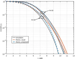
Fig. 3 depicts the CCDFs of PAPR versus λ (in dB), for (a) N =16, 32 subcarriers, and (b) N =64, 128 subcarriers. For each subcarriers number configuration, three curves are compared: one obtained through simulations, and two obtained from theory, referred as ”usual” in (2), and ”proposed” in (12). It can be generally observed that the suggested theoretical PAPR CCDF is closer to simulations than the usual one, for any N ∈ {16, 32, 64, 128}. In particular, Fig. 3 shows that at
CCDF (λ) = 10−4, the difference between proposed CCDF and simulation is less than 0.1 dB, whereas compared to (2), it is equal to 1, 0.5, 0.3, and 0.2 for N =16, 32, 64, and 128, respectively. This shows the relevance of the proposed PAPR analysis for N ≤ 128 compared to the usual one. Furthermore, it shows that the larger N , the closer to simulation the CCDFs.
2 3 4 5 6 7 8 9 10 11 12 λ (dB) 10-4 10-3 10-2 10-1 100 CCDF( λ ) simulation theory, usual theory, proposed N=32 N=16
(a) CCDF of PAPR versus λ (dB), N =16, 32 subcarriers.
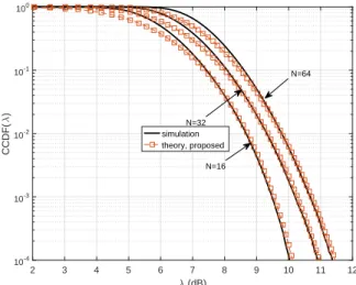
2 3 4 5 6 7 8 9 10 11 12 λ (dB) 10-4 10-3 10-2 10-1 100 CCDF( λ ) simulation theory, usual theory, proposed N=64 N=128
(b) CCDF of PAPR versus λ (dB), N =64, 128 subcarriers. Fig. 3. CCDF of PAPR versus λ (dB), comparison of simulated (exact) CCDF, and usual theoretical CCDF (2) and proposed theoretical CCDF (12), using
N =16, 32, 64, 128 subcarriers.
However, it can be noted that the proposed CCDF does not perfectly match the simulations, in particular in small λ ranges, where it is even slightly worse than CCDF in (2). This is mainly due to the approximation made in (10).
Fig. 4 shows the mean and variance of PAPR versus N from 16 to 2048. Theoretical results in (17) and (20) are compared with those obtained through simulations. It can be clearly observed that µP AP R tends to γ + ln(N ), and νP AP R
tends to π62 as N increases. This shows the relevance of the asymptotic mean and variance analysis of PAPR, and then confirms the results presented in [13].
2) Oversampled Signal: It must be emphasized that
pre-vious developments and results have been presented for multicarrier signals sampled at Nyquist rate. However, for more practical scenarios, the PAPR of oversampled signal should be considered. In order to fit oversampled signals with low subcarriers number, we propose two approximations of
CCDF (λ):
• Van Nee based approximation [2], i.e. N is substituted by
200 400 600 800 1000 1200 1400 1600 1800 2000 N 0 1 2 3 4 5 6 7 8 9
mean and variance of PAPR
µ PAPR = γ + ln(N) µ PAPR, simulations ν PAPR = π 2/6 ν PAPR, simulations
Fig. 4. Mean and variance of PAPR versus N for N =
16, 32, 64, 128, 256, 512, 1024, 2048, comparison between (17), (20), and simulations.
⌊αN⌉ in (12), where ⌊.⌉ is the nearest integer function.
In that case, the coefficient α is empirically set in order to fit the curves obtained by simulation. In the following, this approximation is referred as ”adapted”, since it is adapted from Van Nee approach in [2].
• Proposed approximation, where ˜λ is substituted by ˘λ = βλ
1−βλN in (12), where β is a parameter which is empirically
set. In the following, this approximation is referred as ”proposed”.
Furthermore, we compared the suggested approximation with CCDF expressions derived in the literature [4], [6], [7]. In [4], the authors expressed the CCDF of PAPR as:
CCDF (λ) = 1− exp ( −Ne−λ √ πλ 3 ) . (21)
In [6], [7], the authors based their developments on extreme value theory. The CCDF in [7] is expressed as
CCDF (λ) = 1− exp ( −Ne−λ √ π log(N ) 3 ) , (22)
and this result has been extended in [6] to more a realistic model where subcarriers may not be active, and with different power distribution. In that more general case, the CCDF of PAPR can be written as
CCDF (λ) = 1− exp ( −2Ke−λ √ 2ρπλK 3N ) , (23)
where K is half the number of activated subcarriers, and ρ is related to the power allocation.
In order to validate the suggested approximations, Figs. 5 and 6 show the CCDFs of PAPR versus λ for adapted and proposed approximations, respectively. The oversampling rate is equal to 20, then the PAPR of the signal is very close to that of the continuous signal. In Fig. 5, Van Nee based adaptation has been carried out with α = 1.5. Furthermore,
2 3 4 5 6 7 8 9 10 11 12 λ (dB) 10-4 10-3 10-2 10-1 100 CCDF( λ ) simulation theory, adapted theory, original N=16 N=32 N=64
Fig. 5. CCDF of PAPR versus λ (dB) of oversampled OFDM signal using Van Nee based approximation. The ”original” corresponds to Nyquist rate model in (12). The results have been obtained with an oversampling rate of 20, α = 1.5.
the curve referred as ”theory, original” corresponds to the multicarrier signal with N = 16, and sampled at Nyquist rate such as proposed in (12). It can be seen that the CCDF in (12) underestimates the actual CCDF of oversampled signal of about 0.4 dB. In addition, the Van Nee approximations do not perfectly match the curves obtained through simulations. Thus, a specific α value should be set for every N value.
In Fig. 6, the proposed CCDF approximation has been carried out with β = 0.92. In that case, it can be observed that the proposed CCDFs match well the curves obtained through simulations for CCDF (λ)≤ 0.1. However, it must be noted that further simulations (not shown here) revealed that this approximation does not hold anymore for N > 128 with
β = 0.92 (β should then be adapted), whereas Van Nee’s does
with α = 2.8 such as suggested in [2]. Thus, we can conclude that Van Nee’s approximation can still be used for oversampled multicarrier signals with large N number (N ≥ 128), whereas the proposed one fits signals with low N number (N < 128), even though it can also be used for larger N by adapting β value.
Fig. 7 compares the CCDF of PAPR of the proposed approximation with those of the aforementioned state-of-the-art [4], [6], [7], using a 16-QAM and the same oversampling rate as previously. The CCDF obtained through simulations has been plotted as a reference. Two subcarriers numbers are considered: N =16, in Fig. 7-(a), and N = 64 in Fig. 7-(b). The curve of CCDF corresponding to (23) has been obtained by considering that all subcarriers are active, i.e. K = N2. Note that in the case where ρ = 1, then (23) reduces to (21). Therefore, we arbitrarily set ρ = 0.6 to distinguish (23) and (21). It can observed in Fig. 7-(a) that the proposed approximation almost match the simulations, whereas the three other approximations deviate from simulation for λ ≥ 7 dB. However, in Fig. 7-(b), all the approximations are closer to the simulation. In particular, it is highlighted that, at
CCDF (λ) = 0.0001, the proposed approximation, (22), and
2 3 4 5 6 7 8 9 10 11 12 λ (dB) 10-4 10-3 10-2 10-1 100 CCDF( λ ) simulation theory, proposed N=16 N=32 N=64
Fig. 6. CCDF of PAPR versus λ (dB) of oversampled OFDM signal using proposed approximation. The results have been obtained with an oversampling rate of 20, β = 0.92.
(23) are less than 0.2 dB far from the simulation. This shows the relevance of the suggested analysis and the general CCDF of PAPR expression (12) for low subcarriers number N < 64.
B. Discussion
The various simulations results show the relevance of the suggested general expression of CCDF of PAPR, in particular for low subcarriers numbers 12 ≤ N ≤ 64. However, it can be noted that (12) involves the derivation of two binomial coefficients per element of the sum. Therefore, the calculus of (12) may be not tractable in practice. In fact, if N is higher than 128, the derivation of the binomial coefficients exceeds the computing capacity of most of the present computers. However, it can be noted that ΘN in (9) quickly converges
towards N1(γ + ln(N )) (this is not proved in this paper), which reduces the computation cost of the CCDF for N > 32. Otherwise, computation tricks should be used to obtain the binomial coefficient in (12), e.g. by considering logarithmic additions instead of multiplications.
In practice, we conclude from the different simulations results that (12) should be used for very low subcarriers number, typically N < 128 at Nyquist rate, and N < 64 for oversampled signals. For higher N values, other approxima-tions [2], [4], [6], [7] can be considered for simplicity matter.
VI. CONCLUSION
In this paper, we presented a new and general expression of PAPR CCDF for multicarrier systems, which holds for large and low subcarriers number values, down to N ≥ 12. This formula has been derived by considering the denominator of PAPR as a random variable, whereas it is usually assumed to be a constant. This led us to derive an original distribution function for this denominator. In addition, we showed that an asymptotic analysis of the PAPR leads to the existing results in the literature, in terms of CCDF, mean, and variance of PAPR. These developments, supported by various simulations results,
2 3 4 5 6 7 8 9 10 11 12 λ (dB) 10-4 10-3 10-2 10-1 100 CCDF( λ ) simulation theory, proposed theory, Ochiai et al. [4] theory, Wei et al. [7] theory, Jiang et al. [6]
(a) CCDF of PAPR versus λ (dB), N =16 subcarriers.
2 3 4 5 6 7 8 9 10 11 12 λ (dB) 10-4 10-3 10-2 10-1 100 CCDF( λ ) simulation theory, proposed theory, Ochiai et al. [4] theory, Wei et al. [7] theory, Jiang et al. [6]
10.5 11 11.5 12 10-4
10-3
(b) CCDF of PAPR versus λ (dB), N =64 subcarriers.
Fig. 7. CCDF of PAPR versus λ (dB), comparison of simulated (exact) CCDF, proposed approximation, and CCDF (21), (22), and (23) in [4], [7], and [6], using N =16, 64 subcarriers.
validate the theoretical analysis. Furthermore, we discussed the issue of PAPR of oversampled signals with low subcarriers number, and we suggested an original approximation of PAPR CCDF for such signals. Future works will deal with more practical applications of the presented analysis, considering signals with low subcarriers number such as NB-IoT.
APPENDIX
A. Proof of (8)-(9)
Let ΩX ={X0, X1, .., XN−1} be a set of N independent
zero-mean complex white Gaussian variables with variance
σ2=E{|Xn|2}. Then, the sum Z = N1
∑N−1
n=0 |Xn|2 obeys a χ2 distribution with 2N degrees of freedom and parameter
σZ2 (due to the fact that Xn are not normalized), i.e. the
distribution of Z is written as fZ(z) = NN σ2N Z Γ(N ) zN−1e− N z σ2Z, (24)
where the parameter σZ2 can be straightforwardly deduced from (24). In fact, on one hand, we have
E{Z}= 1
N N∑−1
n=0
E{|Xn|2} = σ2, (25)
and, on the other hand, by property of random variables featuring continuous density functions, it can be shown that
E{Z}= ∫ +∞
0
zfZ(z) = σZ2, (26)
which yields σZ2 = σ2. Note that the latter feature holds for
any degree of χ2 distribution. Thus, suppose that Xi, i ∈
J0, N − 1K, is randomly chosen in ΩX, and let Z′ be defined
as Z′ = Z−|Xi|2
N . Then Z′obeys a χ
2distribution with 2N−2
degrees of freedom with parameter σ2
Z′ = E { Z−|Xi|2 N } = N−1 N σ 2.
Now, suppose that Xi is chosen such that|Xi|2=|Xi,m|2,
where|Xi,m|2 = max i∈J0,N−1K|Xi|
2 (the subscript m points out
that |Xi,m|2 is the maximum value). Then, the variable Y = Z−|Xi,m|2
N still obey a χ
2 with 2N− 2 degrees of freedom
with new parameter σ2Y, which is derived below. It must be noted that the distribution of X = |Xi,m|2 is given in (7),
therefore the value of σY2 is derived as follows:
σ2Y =E{Z−|Xi,m| 2 N } = σ2− 1 N ∫ +∞ 0 xfX(x)dx. (27)
Then, the binomial theorem applied to fX(x) leads to
fX(x) = N σ2(1− e − x σ2)N−1e− x σ2 = N∑−1 k=0 ( N− 1 k ) (−1)kN σ2e −(k+1)x σ2 . (28)
Therefore, substituting (28) into (27) yields
σY2 = σ2− 1 N ∫ +∞ 0 N∑−1 k=0 ( N− 1 k ) (−1)kxN σ2 e −(k+1)x σ2 dx. (29) Then we substitute w = (k+1)xσ2 to recognize the Gamma
function, which finally leads to (9), and then concludes the proof.
B. Proof of (17)
We use the following equivalence (Nk) ∼ Nk!k to simplify
µP AP R in (17): µP AP R∼ − N ∑ k=1 (−1)kNk kk! . (30) Let E1(z) = ∫+∞ z e−t t dt, z ∈ C\R−, be the exponential
integral function, defined in [12]. The series representation of E1 is
E1(z) =−γ − ln(z) − +∞ ∑ k=1 (−1)kzk kk! . (31) Since lim
z→+∞E1(z) = 0, and reminding that N → +∞, then
the substitution of z by N in (31) leads to µP AP R in (17),
which concludes the proof.
C. Proof of (19)
Similarly to the reasoning in Appendix B, it should be first noticed that the first line in (19) becomes
˜ νP AP R∼ −2 N ∑ k=1 (−1)kNk k2k! . (32)
Then, we use the series expansion of the so-called generalized integro-exponential function (see (2.3) and (2.10) in [14]), denoted by Esj, such as hereby described:
Esj(z) = 1 Γ(j + 1) ∫ +∞ 1 ln(t)jt−se−ztdt = +∞ ∑ k=0 k̸=s−1 (−z)k (s− 1 − k)j+1k! +z s−1(−1)j+s (j + 1)! j+1 ∑ k=0 ( j + 1 k ) ln(z)1+j−kΨk,s, (33) where Ψk,s is the polygamma function [11], whose analytical
values are provided in [14], Table 1, and in [15]. It can be noticed that, when s = j = 1:
E11(z) = +∞ ∑ k=1 (−1)kzk k2k! + 1 2 2 ∑ k=0 ( 2 k ) ln(z)2−kΨk,1, (34) where Ψ0,1= 1 Ψ1,1= γ Ψ2,1= γ2+ π2 6 . (35)
From the integral form of Ej
s(z) in (33) we have
lim
z→+∞E
1
1(z) = 0. Then considering z = N and substituting
(32) into (34) finally leads to
˜
νP AP R∼ π2
6 + (γ + ln(N ))
2, (36)
which concludes the proof.
REFERENCES
[1] G. Wunder, R. F. H. Fischer, H. Boche, S. Litsyn, and J.-S. No, “The PAPR Problem in OFDM Transmission: New Directions for a Long-Lasting Problem,” IEEE Signal Processing Magazine, vol. 30, no. 6, pp. 130 – 144, October 2013.
[2] R. Van Nee and A. De Wild, “Reducing the peak-to-average power ratio of OFDM,” in proc. of VTC’98, Ottawa, Ont., Canada, May 1998. [3] R. Van Nee and R. Prasad, OFDM for wireless multimedia
communica-tions. Artech House, January 2000.
[4] H. Ochiai and H. Imai, “On the Distribution of the Peak to Average Power Ratio in OFDM Signals,” IEEE Transactions on Communications, vol. 49, no. 2, pp. 282 – 289, February 2001.
[5] M. Sharif, M. Gharavi-Alkhansari, and B. H. Khalaj, “On the Peak to Average of OFDM Signals Based on Oversampling,” IEEE Transactions
on Communications, vol. 51, no. 1, pp. 72 – 78, January 2003.
[6] T. Jiang, M. Guizani, H. Chen, W. Xiang, and Y. Wu, “Derivation of PAPR Distribution for OFDM Wireless Systems Based on Extreme Value Theory,” IEEE Transactions on Wireless Communications, vol. 7, no. 4, pp. 1298 – 1305, April 2008.
[7] S. Wei, D. L. Goeckel, and P. E. Kelly, “A modem extreme value theory approach to calculating the distribution of the peak-to-average power ratio in OFDM systems,” in proc. of ICC’02, New York, NY, April-May 2002, pp. 1686 – 1690.
[8] 3GPP, “3GPP TS 36.211, Physical channels and modulation (Release 14),” 3GPP, Tech. Rep., March 2017.
[9] A. Rudzi´nski, “Normalized Gaussian Approach to Statistical Modeling of OFDM Signals,” Journal of Telecommunications and Information
Technology, vol. 1, no. 1, pp. 54 – 61, January 2014.
[10] B. Farhang-Boroujeny, “OFDM Versus Filter Bank Multicarrier,” IEEE
Signal Processing Magazine, vol. 28, no. 3, pp. 92 – 112, May 2011.
[11] M. Abramowitz and I. Stegun, Handbook of Mathematical Functions
with Formulas, Graphs, and Mathematical Tables. Ney York: Dover, 1970, ch. 6: Gamma Function and Related Functions, pp. 258 – 266. [12] ——, Handbook of Mathematical Functions with Formulas, Graphs,
and Mathematical Tables. Dover, 1970, ch. 5: Exponential Integral and Related Functions, pp. 227 – 237.
[13] H. Ochiai and H. Imai, “Peak-Power Reduction Schemes in OFDM Systems : A Review,” in proc. of WPMC’98, 1998, pp. 247 – 252. [14] M. S. Milgram, “The Generalized Integro-Exponential Function,”
Math-ematics of Computation, vol. 44, no. 170, pp. 443 – 458, April 1985.
[15] I. K. Abu-Shumays, “Transcendental Functions Generalizing the Ex-ponential Integrals,” Northwestern University, Evanston, Illinois, Tech. Rep., November 1973.
![Fig. 7. CCDF of PAPR versus λ (dB), comparison of simulated (exact) CCDF, proposed approximation, and CCDF (21), (22), and (23) in [4], [7], and [6], using N=16, 64 subcarriers.](https://thumb-eu.123doks.com/thumbv2/123doknet/8234425.276940/8.918.98.418.96.323/ccdf-papr-versus-comparison-simulated-proposed-approximation-subcarriers.webp)
