Numerical Simulation of Light Scattering of a pendent droplet by Statistics Vectorial Complex Ray Model

(1)

HAL Id: tel-02623834

https://hal.archives-ouvertes.fr/tel-02623834

Submitted on 26 May 2020

HAL is a multi-disciplinary open access

archive for the deposit and dissemination of sci-entific research documents, whether they are pub-lished or not. The documents may come from teaching and research institutions in France or abroad, or from public or private research centers.

L’archive ouverte pluridisciplinaire HAL, est destinée au dépôt et à la diffusion de documents scientifiques de niveau recherche, publiés ou non, émanant des établissements d’enseignement et de recherche français ou étrangers, des laboratoires publics ou privés.

droplet by Statistics Vectorial Complex Ray Model

Ruiping Yang

To cite this version:

Ruiping Yang. Numerical Simulation of Light Scattering of a pendent droplet by Statistics Vectorial Complex Ray Model. Physics [physics]. Université de Rouen, 2019. English. �tel-02623834�

(2)

THESIS

For the degree of Doctor of Philosophy

Specialty: Physics

Prepared at the University of Rouen Normandy

Title of the thesis

Numerical Simulation of Light Scattering of a pendent droplet by Statistics Vectorial Complex Ray Model

Presented and defended by

Ruiping YANG

Thesis defended publicly on 12 December 2019 before the jury composed of

Fabrice LEMOINE Professor at ENSEM LEMTA CNRS UMR 7563, University of Lorraine Reviewer Fabrice ONOFRI Director of research IUSTI CNRS UMR 7343, Aix-Marseille University Reviewer Loïc MÉÈS Research fellow at LMFA CNRS UMR 5509, Ecole Centrale de Lyon Examiner François-Xavier Professor at University of Rouen Normandie, CORIA-UMR 6614, Rouen Examiner DEMOULIN

Claude ROZÉ Professor at University of Rouen Normandie, CORIA-UMR 6614, Rouen Co-supervisor Kuan Fang REN Professor at University of Rouen Normandie, CORIA-UMR 6614, Rouen Supervisor

(3)

(4)

Pour obtenir le diplôme de doctorat

Spécialité : Physique

Préparée au sein de l’université de Rouen Normandie

Titre de la thèse

Simulation Numérique de Diffusion de la lumière par une Goutte Pendante par Tracé de Rayons Vectoriels Complexes Statistiques

Présentée et soutenue par

Ruiping YANG

Thèse soutenue publiquement le 12 Décembre, 2019 devant le jury composé de

Fabrice LEMOINE Professeur à ENSEM LEMTA CNRS UMR 7563, Université de Lorraine Rapporteur Fabrice ONOFRI Directeur de recherche IUSTI CNRS UMR 7343, Aix-Marseille Université Rapporteur Loïc MÉÈS Chargé de recherche au LMFA CNRS UMR 5509, Ecole Centrale de Lyon Examinateur François-Xavier Professor at University of Rouen Normandie, CORIA-UMR 6614, Rouen Examiner DEMOULIN

Claude ROZÉ Professeur à l’Université de Rouen Normandie, CORIA-UMR 6614 Codirect. de thèse Kuan Fang REN Professeur à l’Université de Rouen Normandie, CORIA-UMR 6614 Directeur de thèse

(5)

(6)

Acknowledgements

The thesis received funding from the China Scholarship Council. This work was also partially supported by the CRIANN (Centre Régional Informatique et d’Applications Numériques de Normandie).

I have to thank many people who have offered me assistance and encouragement. First and foremost, I would like to express my heartfelt gratitude to my supervisor, Professor Kuan Fang REN, who has spent much time to reading every version of the drafts of my thesis and provided me with invaluable suggestions and excellent guidance. He taught me a effective methodology to carry out scientific research, as an example my major physics. It starts with having a good knowledge of the fundamental physics principles and list systematically the research ideas. Then, it is crucial to design and debug the program according to the physical principles. After that, it is necessary to analyze the obtained simulation results and explain whether the simulation results are reasonable or not based on the physics theory. At last, it is essential to present the research results in a suitable form. With his illuminating instruction, I can achieve the initial simulation results of my program and initially finish the writing of this thesis. The experience I obtained will be of great importance to my future work and study.

Secondly, I owe my particular thanks to my co-supervisor Professor Claude ROZÉ for his code on the SVCRM which has permitted the calculation of the scattering intensity and his software for image processing which extracts the profile of a droplet from the experimental recoded images. It is based on his code of SVCRM I could achieve the work of my thesis. His professional knowledge on SVCRM provides me with theoretical guidance to deal with the light scattering of a pendent droplet in three dimensions. He also introduced some tools that help me manage orderly my program. In addition, his every recognition and encouragement gave me more confidence to continue the research of SVCRM.

Thirdly, thanks go particularly to Driss ABDEDDAIM, student at EsiTech, for the droplet images and the scattering patterns he recorded during his internship at CORIA in 2016 and Romain ALLEAUME, student at Rouen university, for the experimental results (droplet images and the scattering patterns) he recorded during his internship at CORIA in 2017. A special thanks to Saïd IDLAHCEN, engineer of research in CORIA, for his technical support and help in the realization of the experiment on the generation of the droplet, the design of optical system, the acquisition of the image and

(7)

the scattering patterns.

Thanks are also due to the members of the jury, Professor Fabrice LEMOINE, Dr. Fabrice ONOFRI, Dr. Loïc MÉÈS and Professor François-Xavier DEMOULIN for their patience in reading this manuscript and evaluating it.

Finally, I would like to thank my family and boyfriend for their accompany, encourage-ment and support. They share with me my worries, depression, and happiness, which make me feel that I am not alone.

(8)

List of Symbols and Abbreviations

Greek Symbols

α : size parameter of particle

ρ : curvature radius of particle surface

θi : incident angle θr : reflection angle θt : refraction angle θB : Brewster’s angle θC : Critical angle

κ : curvature of a wave front or of particle surface

δ : rotation angle of a general matrix to a diagonal matrix

ϕ : azimuthal angle

θ : polar angle

ϕd : detection azimuthal angle relative to xz plane θd : detection angle relative to the horizontal plane σ0 : initial phase of a ray

σ : phase of a ray

σF : phase shift duo to reflection deduced by Fresnel coefficients σP : phase shift due to optical path

σf : phase shift due to focal lines/points

σX,p : phase of the ray of order p with X polarization Θ : projection matrix

(11)

Romain Symbols

a : radius of a sphere ˜

A : complex amplitude

C : curvature matrix of particle surface

E : electric field

H : height of droplet

l : distance between two successive interaction points within a particle

I : intensity of scattered wave(with interference)

Ino : intensity of scattered wave without interference

k : wave number

k : wave vector of a ray

m : relative refractive index

m0 : refractive index of the surrounding medium mp : refractive index of particle

n : unit vector normal to the particle surface

Nf : total number of focal lines of a ray N : number of emitted photons in SVCRM

OC : center of droplet we set in SVCRM

oc : center of laser source in droplet coordinate system Q : curvature matrix of a wave front

r : Fresnel reflection coefficient

rs : radius of laser source R : reflectivity

T : transmissivity

t : Fresnel refraction coefficient

u : principal curvature direction of a curved surface

(12)

Superscripts and Subscripts

c : for center of light source

C : for center of droplet

s : for coordinates of a point on the light source plane (i) : for incident ray

(r) : for reflection ray (t) : for transmitted ray (s) : for particle surface

i : direction perpendicular to the incident plane

j : direction parallel to the incident plane

1 : principal direction parallel to the equatorial plane 2 : principal direction perpendicular to the equatorial plane

p : order of a ray

(13)

Abbreviations

DDA : Discrete Dipole Approximation FDTD : Finite Difference Time Domain FEM : Finite Element Method

LMT : Lorenz-Mie Theory

GLMT : Generalized Lorenz-Mie Theory GO : Geometrical Optics

GOA : Geometrical optics approximation VCRM : Vectorial Complex Ray Model

(14)

List of Figures

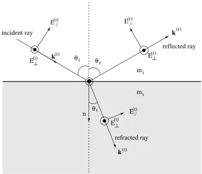
2.1 Directions and electric vectors of the rays used in Snell laws and Fresnel

formulas. . . 21

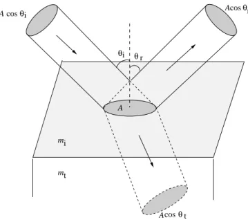
2.2 Energy flux of light during the reflection and the refraction with an oblique incidence . . . 23

2.3 Fresnel coefficients as function of incident angle θi for the relative refrac-tive index m = 1.333 and 0.75. . . . 25

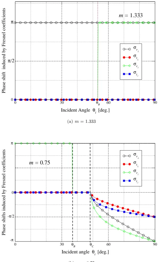
2.4 Phase shifts of the reflected and refracted rays on the surface (a): from air to water and (b): from water to air . . . . 26

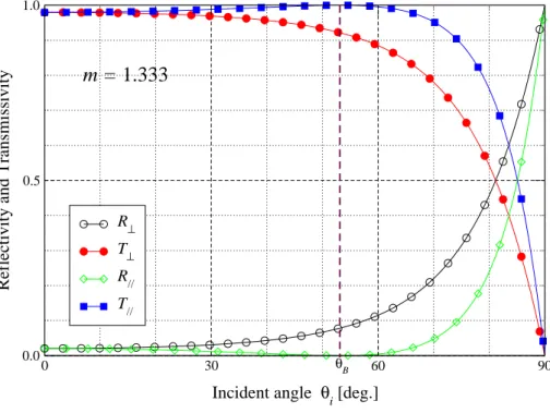
2.5 Reflectivity and transmissivity as function of incident angle θi for two relative relative refractive indice. . . 28

2.6 Schema of light interaction with a large sphere according to Geometrical optics . . . 29

2.7 Ray tracing by GO for a sphere (m = 1.333) illuminated by a plane wave. For clarity, only the above half of the sphere is considered with p = 3. . . . 36

2.8 Scattered intensity of each order of rays and the total intensity (plane wave λ = 0.6328 µm, sphere: m = 1.333 and a = 100 µm). . . . 37

2.9 Scattering diagrams simulated by GO for a sphere (m = 1.333 and a = 100 µm) by a plane wave of wavelength λ = 0.6328 µm with various polarization states . . . 39

2.10 Scattering diagrams simulated by GO for a sphere (m = 1.333 and a = 20 µm) by a plane wave of wavelength λ = 0.6328 µm with various polarization states . . . 40

3.1 Schematic diagram of the wave fronts of the waves before and after interaction and the dioptry particle surface . . . 44

3.2 Variation of pencil cross section . . . 46

3.3 Schematic diagram of interactions between a ray and an irregular particle. 48 3.4 Definition of the direction of various components in Snell-Descartes Laws 51 3.5 Conversion of matrices between different bases . . . 53

3.6 Path of a light ray through a non-spherical particle . . . 59

3.7 Definition of the signs of the curvature radii . . . 61

4.1 Experimental setup systems . . . 66

4.2 Schematic diagram of the experimental setup systems . . . 67 7

(15)

4.3 Experimental images of four pendent droplets and their scattering pat-terns around the rainbow angles with a perpendicularly polarized plane wave (λ = 0.6328 µm). Detection angle in horizontal direction is about

[70◦, 170◦] and that in vertical direction is about [−40◦, 40◦]. . . 68

4.4 Scattering pattern (zones) of a pendent droplet with a perpendicularly polarized plane wave (λ = 0.6328 µm). Detection angle in horizontal direction is about [100◦, 150◦] and that in vertical direction is about [−40◦, 40◦]. . . 70

4.5 Forward scattering pattern of a pendent droplet with a perpendicularly polarized plane wave (λ = 0.6328 µm). Detection angle in horizontal direction and in vertical direction are both about [−45◦, 45◦]. . . 71

4.6 Half of the pendent droplet profile in Cartesian coordinate systems. . . 71

4.7 Half of the pendent droplet profile before and after fitted by Least Squares Fitting-Polynomial . . . 73

4.8 Contours of shaped droplets in Cartesian coordinate system . . . 73

4.9 Profiles of droplets in polar coordinate system . . . 74

4.10 Coordinate system of laser source . . . 76

4.11 Half of the pendent droplet profile in polar coordinates . . . 80

4.12 Definition of the detection angle used in SVCRM . . . 83

5.1 Definition of the coordinate systems used in SVCRM . . . 88

5.2 Scattering patterns of a pendent droplet near rainbow angles simulated by SVCRM with the parameters in Tab. 5.1 and the number of emitted photons N = 4_{× 10}7_{. . . .} ₉₀

5.3 Same parameter as Fig. 5.2 except the number of emitted photons N = 4× 108_{. . . .} ₉₁

5.4 Pendent droplet simplified to a sphere or an ellipsoid. . . 92

5.5 Scattering diagrams of a sphere with the same radius as a pendent droplet calculated by software VCRMll2D. The figures on the right are just a zoom on the first rainbow in the figure on the left. . . 93

5.6 Scattering diagrams of a ellipsoid with the same semi-axes of a pendent droplet calculated by software VCRMll2D. The figures on the right are just a zoom on the first rainbow in the figure on the left. . . 94

5.7 Influence of detection steps on the scattering patterns without inter-ference near the equatorial plane of the pendent droplet a with the parameters in Tab. 5.3 with Ze = 592.54. . . . 96

5.8 Same as Fig. 5.7 but with interference. . . . 97

5.9 Same as Fig. 5.7 but for droplet d . . . . 99

5.10 Same as Fig. 5.9 but with interference. . . . 100

5.11 Scattering patterns without interference of the pendent droplet a with parameters given in Tab. 5.4 and Re= 541.15 µm, H = 989.86 µm. The 9 images correspond to the simulation with 9 pairs of detection steps (Cϕ, Cθ) given in Tab. 5.4 . . . 103

(16)

5.13 Same as Fig. 5.11 but for the droplet d with Re = 671.16 µm and

H = 1707.68 µm . . . . 105

5.14 Same as Fig. 5.13 but with interference. . . 106

5.15 Same parameters as the last images in Fig. 5.14 but the number of photons is N = 2_{× 10}9_{. . . .} ₁₀₇

5.16 Scattering patterns of the reduced droplets a (top) and d (bottom) with the parameters in Tab. 5.6. . . 109

5.17 A schematic to show a droplet is illuminated by a rectangular top-hat beam in 8 different regions. . . 111

5.18 Scattering patterns without interference when the droplet a is illu-minated by a thin rectangular to-hat beam at different. The detection step Cθ = 0.05 and the other parameters are given in Tab. 5.7. . . . 112

5.20 Same as Fig. 5.18 but for droplet d. . . . 114

5.21 Same as Fig.5.18 but with interference. . . . 115

5.22 Scattering patterns without interference around the rainbow angles of the 4 droplets with the parameters in Tab. 5.8. . . 117

5.24 Scattering patterns without interference in forward direction of the 4 droplets with the parameters in Tab. 5.9. . . 120

5.25 Scattering patterns with interference in forward direction of the 4 droplets with the parameters in Tab. 5.9. . . 121

5.26 Scattering patterns without interference (left) and with interfer-ence (right) in the forward direction of the droplet d. The detection region is ϕ∈ [−10◦, 10◦] and θ∈ [−30◦,−20◦]. . . 122

(17)

(18)

List of Tables

4.1 Coefficients of the 10th _{degree polynomials for shaped droplets. . . .} ₇₄

4.2 Parameters of the four droplets in Fig. 4.3. . . 83 5.1 Parameters for the preliminary simulation of the scattering intensities

with and without interference. . . 89 5.2 Detection steps of angle ϕ for the sphere and the ellipsoid simplified from

the droplet a and the droplet d. . . . 95 5.3 Parameters for the scattering intensity near the equatorial plane of droplet 98 5.4 Various detection steps for the scattering intensity of droplet around the

rainbow angles. . . 101 5.5 Parameters for the scattering patterns around the rainbow angles with

different detection steps. . . 101 5.6 Parameters for the calculation of the scattering patterns of the reduced

droplets. . . . 108 5.7 Parameters for the calculation of the scattering patterns of partially

illuminated droplets. . . 110 5.8 Parameters for the simulation of scattering patterns around the rainbow

angles of the 4 droplets. . . 116 5.9 Parameters for the calculation of the scattering patterns droplets in the

forward direction. . . 119

(19)

(20)

Chapter 1 Introduction

The light scattering is omnipresent in our daily life, in the industrial processes and in many domains of scientific research. For instance, the wavelength dependence of the light extinction in the atmosphere permits to understand why the sky is blue and the sun looks red at sunrise and sunset [1]. The dispersion of the refractive index of water and the refraction of the light in water droplets can be used to explain the disposition of the colors in the rainbows [2]. The on-line control of the diameter of an optical fiber can be realized by simply measuring its scattering properties. We can also have access to the temperature, the sizes and the velocities of droplets in combustion chambers via the signals of light scattered by these droplets, etc. These understandings and the realizations are possible only when the relation between the morphological and material properties of the scatterers and its scattering properties is established. That is just the role of the light scattering theories and the models.

The scientists have been working on this subject for centuries and have developed various theories and models which can be classified into three categories. The first is the rigorous theories which are the exact solutions of the Maxwell equations, such as the Lorenz-Mie theory (LMT) [3, 4] and its generalizations (GLMT)[5, 6]. They are applicable only to particles of simple shapes [7], i.e. the shape of the scatterer must correspond to a mathematical coordinate system (sphere [8], spheroid [9], ellipsoid, circular [10] and elliptical infinite cylinder [11], ...). Though these theories are very limited in the shape of the scatterer, their results serve usually as reference to validate other models and methods. However, except for the homogeneous or stratified sphere and the circular infinite cylinder[12], the calculable size of these theories is often limited to some tens of wavelengths[7, 13] due to the problem of numerical calculation of the involved special functions.

The second category is the numerical methods, which solve the scattering problems nu-merically with help of the powerful computation resources. For example, T-Matrix [14, 15] solves the electromagnetic scattering using a transformation matrix. Sanamzadeh et al present a solution to a dielectric layered medium with random rough interfaces.

(21)

Martin[16] developed a new method for calculating T-matrix of two aspheric obstacles. The T-matrix can also be applied to the calculation of radiation forces. Reference [17] discusses the change of non-radial radiation pressure under the interaction of differ-ent chemical composition and spatial arrangemdiffer-ent of grain with sunshine. The discrete dipole approximation (DDA) [18, 19, 20] and the finite-difference time-domain (FDTD) [21, 22, 23] can predict the scattering of particles of complex shapes. Yukin, for instance, developed ADDA [24, 20] to speed up the DDA code. But in general, the size of the particles can be calculated with the numerical methods is very limited, it does not exceed few and to a few a hundred wavelengths.

The last category is the approximate models which can be applied to deal with the scattering of particles of irregular shape, but their precision is often not sufficient. As an example, Rayleigh model [25, 26] is a good approximate model for the particles of size much smaller than the wavelength, i.e. a ≪ λ with a the radius of the particle and λ the wavelength. It predicts that the extinction factor of very small particle is proportional to 1/λ4_{, i.e. the extinction of the red light through the atmosphere is much}

smaller than the blue one, which answers the question the colors about the sky and the sunset. Conversely, the Geometrical Optics (GO) can only deal with the scattering of large particles of dimension much larger than the incident wavelength, i.e. a ≫ λ. Van de Hulst [27] firstly considered the Geometrical optics approximation (GOA) for the scattering of a spherical particle illustrated by a plane wave in detail, which in-cludes the light intensity, phases and two sets of focal lines of optics rays. Extension of geometrical-optics approximation to on-axis Gaussian beam scattering by a spherical particle[28] or a spheroidal particle with end-on incidence[29]. The light scattering of large air bubbles by Geometrical optics approximation is investigated with the relative refractive index smaller than 1 by taking the total reflection into consideration[30]. For this case, Hovenac and Lock [31] proposed that the particle diameter needs to be an order of magnitude larger than the wavelength. GOA is employed for the light scat-tering by absorbing spherical particles [32], considering spherical particles of different absorption properties. The agreement of scattered light with GOA and LMT is better for larger particles than smaller particles. In addition, the calculation speed of the GOA is independent of the particle size while that of LMT becomes slow with the particle size increasing, which presented GOA is more efficient than LMT for particles. In addtion, GOA has been developed to analyze the scattering of irregular particles. A geometrical-optics approach is also used to deal with the scattering of nonuniform glass microbeads illuminated by on-axis Gaussian beam and comparison of the inten-sity distributions has been obtained by GOA and GLMT [33]. Using the lognormal statistics to generate particles of various random shapes, Ray optics approximation is devoted to the light scattering of Gaussian random particles [34]. Generating randomly shaped particles by cutting an auxiliary random field by a hyperplane, the relation of scattering matrix elements for irregular shaped particles with scattering angle in the GOA is discussed, the differences of which between the indicatrices at infinity and at a close distance noticeably depend on both the particle shape and the distance [35]. Nevertheless, the precision of the geometrical optics is very limited and it is very dif-ficult to take into account the divergence/convergence of a wave on the surface of the

(22)

particle.

In conclusion, none of the aforementioned theories, models or methods can deal with the light scattering of large non-spherical particles with precision. But in practice, we encounter often particles of irregular shapes, such as raindrops in nature, ligament in the atomization or liquid jets in the motor injection. In order to overcome this bottleneck problem, the Vectorial Complex Ray Model (VCRM) [36, 37, 38] for the light scattering by large particles of smooth surface and arbitrary shape has been developed. In this model, all waves are considered as bundles of vectorial complex rays with five parameters: amplitude, phase, direction of propagation, polarization and wavefront

curvature. The ray direction and the wave divergence/convergence after each interaction

of the wave with a dioptric surface as well as the phase shifts of each ray are determined by the vector Snell law and the wavefront equation according to the curvatures of the surfaces. The total scattered field is the superposition of the complex amplitudes of all orders of the rays emergent from the object. Thanks to this simple representation of shaped waves, this model is very suitable for the description of the interaction of an arbitrary wave with an object of smooth surface but complex shape. The application of the model to the scattering of a plane wave by an ellipsoidal particle has been validated numerically [39] and experimentally [40] in the cases a plane of symmetric scattering problems.

In order to extend the applications of the model, we develop algorithms for three dimension objects. VCRM permits to calculate the complex amplitude of each ray but to obtain the total scattering field we must count the contribution of all rays arriving at the same angle. This needs a 2D interpolation of irregular data which is a very difficult and costly task. To get over this obstacle, a statistic version of VCRM, called here after Statistic Vectorial Complex Ray Model (SVCRM), has been proposed and coded by Professor Claude Rozé, in which the total scattered intensity is calculated statistically by summation of the intensity of all rays/photons arriving in boxes in given direction [41]. The scattering patterns simulated by SVCRM agree well with the skeletons of the images obtained experimentally and scattering mechanisms of different orders are identified.

Nevertheless, in its initial version of SVCRM, the interference was not considered. So it cannot predict the fine structure in the scattering patterns. In order to make a complet simulation of the light scattering with SVCRM, the phase of each ray must be counted

and the complex amplitude of the scattered field has to be calculated. This is the main objective of this thesis.

As an example of applications to demonstrate the power of the VCRM/SVCRM, we choose to study the scattering of a water droplet. In one hand, it is easy to be obtained, its property is stable and its surface is naturally smooth. On the other hand, its applica-tion is very broad. For instance, the electric charge of spherical water droplets is evalu-ated for various droplet radii in [42]. The effect of a dense surrounding medium between two approaching charged droplets was studied and the water droplets of precise volume

(23)

inside the dielectric medium can be controlled by changing the electrical forces through adjusting electrical conductivity and obtained by experiments and simulations in [43]. In experiment [44], the effects of electrical conductivity on electrospraying modes and its produced droplets are investigated. The dynamic aspects of droplet behavior under various ambient conditions are described in [45], such as charged droplets, instabil-ity of droplets, evaporation of a single droplet, droplet generation, etc. The highly heterogeneous and unstable temperature and velocity fields of the gas-vapor mixture were observed, and the aerodynamics of the evaporating droplets and the transverse and transverse dimensions of the heat trace lines were determined in [46]. The effect of overheated random Si Nanowires on impacting water droplets is presented and the effects of the surface temperature and impact velocity on the droplet behavior are also presented in [47]. The dynamic process of single water droplets striking the hot oil sur-face at the temperature range of 205◦C to 260◦C is presented in [48]. The behavior of evaporated water droplets on lubricated-impregnated nano-structural surfaces (LINS) was studied experimentally in [49]. The dynamics of non-axis symmetric evaporating droplet with metallic inclusions heated in a high-temperature gas flow is studied in [50]. The impact and freezing process of water droplets was studied experimentally and numerically in [51]. The heating and evaporation of suspended water droplets in a hot air flow are described in [52].

More specifically, we will apply in this thesis our developed model and algorithm to the scattering of the pendent droplets obtained experimentally. Its shape is sufficiently irregular, not as a sphere, a spheroid or an ellipsoid whose surface can be described with a simple mathematical function. The quality of the droplet images and the scattering patterns are sufficiently good for numerical simulation and comparison. The scattering diagrams in three dimension are also very rich in information to be explored.

Finally, we would note that the four terms may be used for the light according to the context: light, wave, ray or photon:

• light is very general, used when we talk about light scattering, interaction of light with particle, etc.;

• wave emphasizes the wave effect, for wavefront, propagation of (light/electromagnetic) wave, divergence or convergence of a wave;

• ray is used in GO, VCRM also in SVCRM. In GO, a ray has four properties: direction, amplitude, polarization state and phase. But it has one more property - wavefront curvature in VCRM and SVCRM.

• photon is used only in SVCRM, which has the same properties as ray (geomet-rical and not its quantum sense).

Therefore, we may talk about the curvature of a ray or a photon, that means just the wavefront curvature of the wave that is described by the ray or the photon.

(24)

The rest of the thesis is organized as follows.

1. Chapter two recalls firstly some fundamentals of Geometrical Optics(GO), in-cluding the Snell-Descartes laws and Fresnel coefficients. We then describe how to deal with the scattering of a homogeneous sphere in the framework of GO. The scattering diagrams calculated by GO are compared with the Lorenz-Mie Theory (LMT) to examine the limitation of the GO that is becoming overwhelmingly complex to deal with the scattering of non-spherical object.

2. Chapter three presents the general principle of the Vectorial Complex Ray Model (VCRM). After that, the Statistical Vectorial Complex Ray Model (SVCRM) is described in detail, for example, how to calculate the complex amplitude of the ray, the total scattered intensity with and without interferences, which is the theoretical guidance for numerical simulation in Chapter 5.

3. Chapter four is devoted to the generation of the pendent droplets and the mathe-matical description of their profiles. The experimental images of the droplets and their scattering patterns are provided which serve to the numerical simulation in Chapter 5.

4. Chapter five compiles the numerical simulation of the scattering patterns of the pendent droplets under different conditions. These results have been analysed and compared with the experimentally recorded scattering patterns to verify the proposed model SVCRM and investigate the scattering mechanism of a pendent droplet. The effect of detection steps, the number of emitted photons, the size of droplets as well as the incident area of photons on the intensity distribution around the rainbow angle are discussed.

(25)

(26)

Chapter 2 Fundamentals of Geometrical

Optics

Geometrical Optics (GO) is an approximate method allowing describing the propaga-tion and interacpropaga-tion of light with objects when the light wavelength λ is much smaller than the dimension of the objects. In this case, the light wave is modelled as rays (pen-cil of light). The wave effects of the light are then ignored. The essential advantage of the GO is its simplicity and flexibility in dealing with the formation of image and the interaction of light with objects, especially when their shapes are not regular.

The Statistical Vectorial Complex Ray Model (SVCRM), an extension of the Vectorial Complex Ray Model (VCRM), developed in this thesis is fundamentally based on the geometrical optics. Therefore, we will recall the fundamentals of GO in this first chapter for two purposes: to define the notations used in next chapters and to introduce

the understanding and analysis of the scattering mechanics.

In the field of theoretical and numerical research on the interaction of light with parti-cles, the scattering of the plane wave by a spherical particle (or a circular cylinder) is the only case we can deal fully with the classical GO. It will be recalled in this chapter to help us to understand the newly developed SVCRM. Some numerical results will be presented also because they will be used later on for the validation of SVCRM in the following chapters.

2.1 Basis of Geometrical Optics

When light travels from one medium to another of different refractive index, reflection and refraction of the light occur. The propagation direction of the light may be deviated. The amplitudes and the phases of the reflected and the transmitted waves change. We recall the Snell-Descartes laws and the Fresnel formulas to describe the relations between

(27)

these parameters and the properties of the media. Numerical results are also given to illustrate the variation of them with the refractive index, the incident angle and the polarization state of the incident wave.

2.1.1 Snell-Descartes laws

Snell-Descartes laws [53] describe the relationship between the directions of the reflected ray and the refracted ray with that of the incident ray when light passes through a interface between two media. The Snell-Descartes laws state also that the incident ray, the reflected ray and the refracted ray are all in the incidence plane which is defined by the incident ray and the normal of the surface. They can be expressed with the following two equations:

θr = θi (2.1) misin θi = mtsin θt (2.2)

where θi, θr and θt are respectively the angles of the incident ray, the reflected ray and

the refracted ray relative to the normal of the interface of the two media, as shown in Fig. 2.1. mi and mt are the refractive indices of the first (incident) and the second

(transmitted) media.

Usually, to simplify the notation, we use the relative refractive index m defined as the ratio of the refractive indices of the two media:

m = mt mi

(2.3) Then the refraction angle θt can be given by:

sin θt = 1 msin θi = 1 m √ 1− cos2_θ i (2.4)

When the light passes from an optically denser medium to a optically light less dense medium, i.e. m < 1, the quantity sin θi/m may be bigger than one. In this case, total

reflection occurs. The limit of the incident angle at which total reflection occurs is called critical angle θC and given by:

θC = arcsin(m) (2.5)

That means all rays with incident angle θi ⩾ arcsin(m) are totally reflected.

2.1.2 Fresnel coefficients

When a wave is incident on an interface plane between two media, a part of the energy is reflected and the other part is transmitted. The amplitudes of the reflected wave and

(28)

the refracted wave with that of the incident wave is given by the Fresnel formulas [53]. Consider an incident wave of electric field E decomposed in two components, one perpendicular to the incident plane E_⊥(i) and the other parallel to the incident plane

E_∥(i) (see Fig. 2.1).

0 0 1 1 0 0 1 1 0 0 1 1 (r) (r) (t) // (t) θt i t (i) (i) E_// k (i) (r) E(t)_// k E E E E k θ θi r n reflected ray incident ray refracted ray m m

Figure 2.1: Directions and electric vectors of the rays used in Snell laws and Fresnel formulas.

We define the ratios of the electric amplitudes of the reflected wave and the transmitted wave to that of the incident wave by

rX = E_X(r) E_X(i) tX = E_X(t) E_X(i) (2.6) where X =⊥ or ∥ stands for the polarization state of the wave. These ratios are called Fresnel coefficients and given by the Fresnel formulas for the perpendicular polarization:

r_⊥= E (r) ⊥ E_⊥(i) = cos θi− m cos θt cos θi+ m cos θt t_⊥= E (t) ⊥ E_⊥(i) = 2 cos θi cos θi + mcos θt (2.7)

(29)

and for the parallel polarization: r_∥ = E (r) ∥ E_∥(i) = cos θt− m cos θi cos θt+ m cos θi t_∥ = E (t) ∥ E_∥(i) = 2 cos θi cos θt+ m cos θi (2.8) It should be noted that when the total reflection occurs, sin θi > m and cos θt becomes

a complex numbers. In this case, the Fresnel coefficients for the total reflection can be expressed as [53]: r_⊥ = cos θi− i √ sin2θi− m2 cos θi+ i √ sin2θi− m2 r_∥ = i √ sin2θi− m2− m2cos θi i√sin2θi− m2+ m2cos θi (2.9) These two coefficients are complex numbers.

We would note also that the reflection coefficients may also be negative. In both cases: the reflection coefficients negative or complex, the reflected wave experiences a phase jump on reflection. This phase shift σF,X can be calculated by the argument of the

reflection coefficient:

σF,X = arg(rX) (2.10)

In the case of parallel polarization, the reflection coefficient r_∥ is zero when cos θt = m cos θi. This special angle of incidence is called Brewster’s angle and is given by:

θB = arctan(m) (2.11)

At this angle, the reflected light is perfectly polarized in the perpendicular direction to the incident plane if the incident light is unpolarized. This property is widely used in optical devices.

2.1.3 Reflectivity and transmissivity

When a wave of light or a bundle of rays arrives on the interface between two media, the incident light generally splits two parts: one is the reflected light and the other the transmitted light. The cross section of the refracted bundle of rays is usually different from that of the incident bundle of rays due to the deviation of the propagation direction. We derive in the following the reflectivity and transmissivity which are the

(30)

cos cos θ θ θ t cos θ m mi t A A A A θr r i i

Figure 2.2: Energy flux of light during the reflection and the refraction with an oblique incidence

ratios of the reflected and transmitted energy flux to the incident one as function of the Fresnel coefficients.

Consider a bundle of rays illuminating an area A on the surface (Fig. 2.2). For a plane wave, the intensity of light being I = ||E × H|| = mE2_{/2 for non-magnetic-dielectric}

medium (here m indicates the refractive index in the medium). The energy flux of the incident light, the reflected light and refracted light on the area are respectively

J(i) = 1 2miE (i)2 cos θi, (2.12) J(r) = 1 2miE (r)2 cos θr, (2.13) J(t) = 1 2mtE (t)2 cos θt. (2.14)

The reflectivity RX and the transmissivity TX are given by RX = J(r) J(i) = micos θr micos θi E_X(r) E_X(i) 2 = cos θr cos θi |rX|2 TX = J(t) J(i) = mtcos θt micos θi E_X(t) E_X(i) 2 = mtcos θt micos θi |t X|2 (2.15) Because θr = θi and mt/mi = m, Eq. (2.15) can be expressed as:

RX =| rX |2 TX = 1− RX = m cos θt cos θi | t X |2 (2.16)

(31)

The above derivation is based on the energy balance on the illuminated area and we have naturally TX + RX = 1. The transmissivity is not equal to the square of the

amplitude ratio of the transmitted wave to the incident wave because the cross section of the transmitted wave is different from those of the incident and reflected waves.

2.1.4 Numerical results and discussions

In this part, numerical results on the Fresnel coefficients, the phase shifts, and the transmissivity and the reflectivity are presented as function of incident angle for different refractive indices with the simulated step of number 300. This investigation provides a concrete understanding of the properties of reflected wave and transmitted wave, and this will be very helpful for the analysis in the following chapters.

The variation of the four Fresnel coefficients are shown in Fig. 2.3 as function of the incident angle for two relative refractive indices, one larger than unit and the other less than 1.

We find that when light passes from an optically looser medium to a denser one (the relative index greater than 1, Fig. 2.3(a)), the two Fresnel coefficients of the transmitted light (red and blue curves) are always positive whatever the state of polarization, the Fresnel coefficient of reflection is always negative for the perpendicular polarization, while that of reflection for parallel polarization is positive when the incident angle is less than the Brewster angle (θB = 53.12◦ for m = 1.333), and negative when the

incident angle is greater than the Brewster angle. This means that the phase of the reflected wave experiences a jump π when the incident angle passes the Brewster angle. When the light passes from an optically denser medium to a looser one (the relative index less than 1, Fig. 2.3(b)), if the incident angle is greater than the critical angle (θC = 48.59◦ for m = 0.75), the Fresnel coefficients of reflection (r⊥ and r_∥) are equal

to unit and those of refraction (t_⊥ and t_∥) are zero, so the total reflection occurs. When the incident angle is less than the critical angle the variation of the Fresnel coefficients are similar to those in the case m > 1. However, it is worth to note that the two Fresnel coefficients of refraction are both greater than 1 and the Fresnel coefficient of reflection for the parallel polarization passes from negative to positive at the Brewster angle (θB = 36.87◦) in the inverse sens to that for m > 1.

The phase shift due to the reflection or refraction can be deduced from the Fresnel coefficient according to Eq. (2.10). The variation of this phase shift as function of incident angle is given in Fig. 2.4 for the two values of refractive index. When the relative refractive index is greater than 1, there is no phase shift for the refracted wave whatever the polarization. The phase shift is also 0 for the perpendicularly polarized reflected wave, while the phase of the reflected wave undergoes a phase jump at Brewster angle.

(32)

0 30 60 90

Incident Angle θ_i[Deg]

-1.0 -0.5 0.0 0.5 1.0 Fresnel coefficients r⊥ t ⊥ r_// t // m = 1.333 θ_B (a) m = 1.333 0 30 60 90 Incident Angle θ i [Deg] 0.0 1.0 2.0 3.0 Fresnel Coefficients r ⊥ t ⊥ r_// t // θ_B θ_C m = 0.75 (b) m = 0.75

Figure 2.3: Fresnel coefficients as function of incident angle θi for the relative refractive

(33)

0 30 60 90

Incident Angle θ

i [deg.]

Phase shift induced by Fresnel coefficients

θ_B σ_r ⊥ σ_t ⊥ σ_r // σ_t // m = 1.333 π 0 π/2 (a) m = 1.333 0 30 60 90

Incident angle θ_i[deg.]

Phase shifts induced by Fresnel coefficients

σ_r ⊥ σ_t ⊥ σ_r // σ_t // m = 0.75 π 0 -π -π/2 θ_B θ_C (b) m = 0.75

Figure 2.4: Phase shifts of the reflected and refracted rays on the surface (a): from air to water and (b): from water to air

(34)

When the relative refractive index is less than 1, the phase shift is much more compli-cated. When the incident angle is less than the critical angle, there is no phase shift for the refracted wave and the reflected wave in perpendicular polarization. The reflected wave in parallel polarization experiences a phase jump equal to π at the Brewster angle. The phase shift varies continuously when the incident angle is greater than the critical angle, i.e. in the total reflection case, the phase shift decreases from 0 at critical angle to −π/2 for refracted wave and to −π for reflected wave at θi = 90◦.

Finally, we show in Fig. 2.5 the reflectivity and the transmissivity as function of incident angle with also two values of relative refractive indice, one greater than unit and the other less than 1. We note simply that the curves for the relative index less than 1 is similar to that for the case m > 1 but compressed to the region of incident angle between 0 and the critical angle. The reflectivity for the perpendicular polarization increases monotonically to 1 at 90◦ for m > 1 and at critical angle for m < 1, while the reflectivity for parallel polarization decreases until 0 at Brewster angle and then increases until 1.

The above analysis provides us a general view about the properties of the reflected wave and the refracted wave as function of incident angle, the state of polarization of the incident wave and the relative refractive index, especially the amplitudes and the phase shifts of the reflected and the refracted waves as well as the reflectivity and transmissivity. On this basis, we will investigate the scattering of a large homogeneous sphere with GO in the following section.

2.2 Geometrical optics for scattering of a sphere

In Geometrical optics, the divergence and the convergence of the wave on the surface of the object is usually not taken into account. However, when dealing with the scattering of light by a sphere, we can not only deduce the four properties of each ray from the fundamental laws given in the previous section, but also obtain an analytical expression of a factor describing the divergence and convergence of a wave on the particle surface and the phase shift due to the focal lines.

This section consists of two parts. First, we will give a general description of how to deal with the scattering problem in the framework of GO, and then some numerical results will be exemplified. The advantages and the limit as well as its precision will be investigated by comparison with Lorenz-Mie theory.

2.2.1 Description of the method

Consider a plane wave of wavelength λ propagating along z axis which illuminates a sphere of real refractive index mp and radius a. The trajectory of a ray is given in

(35)

0 30 60 90

Incident angle θ_i[deg.]

0.0 0.5 1.0

Reflectivity and Transmissivity

m = 1.333 θ_B R_⊥ T_⊥ R_// T_// (a) m = 1.333 0 30 60 90 Incident angle θ i[deg.] 0 0.5 1

Reflectivity and transmissivity

θ_C R_⊥ T_⊥ R_// T_// θ_B m = 0.75 (b) m = 0.75

Figure 2.5: Reflectivity and transmissivity as function of incident angle θi for two

(36)

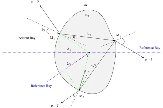
Fig. 2.6. Its interaction position on the sphere is characterized by an angle θi and its

distance from the axis z, which is a cos τ , where τ is the complementary angle of θi, i.e.

angle between the particle surface and the incident ray. Each time a ray interacts with the particle surface, it is split in two parts: the reflected ray and the refracted ray. We call emergent ray of order p,the ray which exits from the particle after p + 1 interactions with the particle surface. Thus, the rays experience a specular reflection on the outer surface of the particle are of order p = 0, the rays exiting after two refractions are of order p = 1, etc. p = 2 p = 1 θ τ τ τ Incident Ray Reference Ray θd o Symmetric axis p = 0 i m t m z ’ t ’ θi

Figure 2.6: Schema of light interaction with a large sphere according to Geometrical optics

Owing to the symmetry of the sphere, the angle of any emergent rays with respect to the normal of the particle surface is constant and equal to the incident angle θi. The

angle between any ray in the particle and the normal of the surface is also constant and equal to the refraction angle θt. Similarly, τ′ is the complementary angle of the

refraction angle1_{. The relation between the incident angle and the refraction angle, or}

equivalently the relation between the angles τ and τ′ is given by the Snell-Descartes law Eq. (2.2):

cos τ′ = 1

mcos τ (2.17) 1_{For convenience we use in this section the angles τ and τ}′ _{instead of θ}

i and θtas in the literature

(37)

Direction of emergent rays

Since the angles of all the emergent rays with respect to the particle surface are constant and the angles of all the rays in the particle make the same angle with the particle surface also, the deviation angle of any emergent ray can be given analytically as function of the incident angle and the refraction angle. For example, the deviation angle θ0 of

the externally reflected ray (p = 0) with respect to the incident direction is 2τ in counterclockwise sense. For the refracted ray, there is a 2τ′ deviation angle in clockwise sens for each interaction. The deviation angle θp of the emergent ray of order p is

therefore:

θp = 2 (τ− pτ′) (2.18)

However, the scattering light is generally observed in the range of [0◦, 360◦]. Partic-ularly, for the scattering of plane wave by a sphere, the scattering angle is usually given in the interval [0◦, 180◦] owe to the symmetry of the problem. In this case, the scattering angle of a ray of order p can be expressed as [3]:

θsp = 2qp(τ − pτ′) + 2kpπ (2.19)

where kp is a integer, which stands for the times that the emergent ray crosses the z

axis, and qp is +1 or−1.

The differentiation of the scattering angle with respect to τ gives

dθsp dτ = 2 ( 1− ptan τ tan τ′ ) (2.20) When the derivative is zero, the scattering angle reaches an extreme value which cor-responds to the geometrical rainbow angle θOG:

θGO(m, p) = 2 arctan   √ m2_{− 1} p2 − m2   − p arctan  p √ m2_{− 1} p2− m2   + qπ (2.21) where q is a integer to be chosen so that θOG ∈ [0, π]. Eq. (2.20) will also be used to

calculate the divergence factor.

Amplitudes of emergent rays

The amplitude of an emergent ray is affected by two factors:

εX,p due to reflection and transmission on the particle surface: this factor depends on

(38)

Dp due to divergence and convergence of the wave: the amplitude of the emergent

wave may be greater or smaller than the incident one depending on the curvature of the particle surface – concave or convex at different interaction points.

The amplitude ratios of the reflected and the transmitted waves to the incident wave at each interaction are given by the Fresnel formulas2_:

r_⊥ = sin τ − m sin τ ′ sin τ + m sin τ′ r_∥ = m sin τ − sin τ ′ m sin τ + sin τ′ (2.22) Since the angles τ and τ′ are constants for all order rays in the scattering of plane wave by a sphere, the amplitude ratio of the emergent rays of order p can be given by these two constant coefficients r_⊥ and r_∥. For example, for the rays of order p = 0, the amplitude ratio of the reflected wave to the incident one is directly the Fresnel coefficient of reflection rX. The rays of order p = 1 experience two refractions (transmissions), so

the amplitude ratio is given by t2

X = 1−r2X. In general, the rays of p≥ 1 experience two

refractions (transmissions) and p−1 reflections on the internal surface of the particle for which the Fresnel coefficient is_−rX calculated by Eq. (2.22). Therefore, the amplitude

ratio of an emergent ray of order p to the incident ray is given by

εX,p= { rX for p = 0, (−rX) p−1( 1− r_X2) for p > 0. (2.23) where, rX is the Fresnel coefficients of reflection for polarization X =⊥, ∥ given in Eq.

(2.22).

When a wave arrives on a curved surface, its wavefront will be changed, i.e. converged or diverged, according to the curvature of the surface. Therefore, the amplitude of the emergent wave per unit surface will increase or decrease. This variation can be described by the divergence factor, which can be derived analytically by the balance of energy for the scattering of a plane wave by a sphere.

Consider a finite pencil of light illuminating the sphere. Let I0 denote the intensity of

the incident light. The illuminated area can be expressed as function of angle increments

dϕ and dτ such that dS = a cos τ dϕ· adτ = a2_{cos τ dτ dϕ. The flux of energy in this}

pencil is therefore I0sin τ dS = I0a2sin τ cos τ dτ dϕ. After successive interactions with

the particle surface, this energy flux in area dS spreads into a solid angle sin θspdθspdϕ,

i.e., over an area dSs = r2sin θspdθspdϕ at a large distance r from the sphere. If we

2_{These two formulas are the same as those given in section 2.1 but as function of the complementary} angles of the incident and refraction angles. The two complementary angles are preferred in the study of the scattering of a plane wave by a sphere, since it simplifies the notation, especially for the deviation angle.

(39)

neglect the energy loss due to absorption and suppose that the intensity of scattered wave of order p at angle θsp is Ix(p, θsp) we will have I0sin τ dS· ε2X = IX(p, θsp)dSs i.e.

IX(p, θsp) = ε2 XI0a2cos τ sin τ dτ dϕ r2_{sin θ} spdθspdϕ = a 2 r2I0ε 2 XDs (2.24) where Ds is called the divergence factor of the wave defined by

Ds = sin τ cos τ sin θsp dθsp dτ = sin 2τ 4 sin θsp 1 − p_{tan τ}tan τ′ (2.25) according to the Eq. (2.20). Then, the divergence factor of the rays of order p can be expressed by the incident θi and refraction angles θt:

Ds= sin 2θi 4 sin θsp ( pcos θi cos θt − 1 ) (2.26) For the rays of low orders, sin θsp can be further expressed as function of the incident θi and refraction angles θt in simple form. For example, the divergence factor of order p = 0 is: Ds0 = sin 2θi 4 sin (π− 2θi) = 1 4 (2.27) since the scattering angle θsp = π− 2θi.

Similarly, we can obtain the divergence factor for p = 1:

Ds1 = sin 2θi 4 sin [2 (θt− θi)] · m cos θt cos θi− m cos θt (2.28) and for order p = 2:

Ds2 = sin 2θi 4 sin [2 (θt− θi)− π] · m cos θt 2 cos θi− m cos θt =− sin 2θi 4 sin [2 (θt− θi)] · m cos θt 2 cos θi− m cos θt (2.29) These analytical expressions are useful to check our code and the divergence factor in VCRM.

(40)

Phase of emergent rays

When the incident wave is a plane wave, its phase is constant. The phase shift of a ray during the interaction with the particle is caused by three facts [3]:

• σP: phase shift due to the optical path,

• σF: phase shift due to reflection and refraction, which can be calculated from the

Fresnel coefficients,

• σf: phase shift due to the focal lines.

The phase of an emergent ray is given by

σp = σP + σF + σf (2.30)

Thanks to the symmetry of the sphere, all the three phase shifts can be expressed analytically as function of the incident angle and the parameters of the sphere.

1. Phase shift due to Fresnel coefficients σF:

This phase shift can be calculated directly by Eq. (2.10). The variation of the phase shift as function of the incident angle has been investigated in the first section in this chapter for the relative reflective index smaller or greater than unity.

In our case of plane wave scattering by a sphere, the total reflection can never occur on the internal surface. The Fresnel coefficients can never be complicated and the phase shift due to the Fresnel coefficient is given according to Eq. (2.23) by σF = arg(εX,p) = { arg(rX) for p = 0, (p− 1) arg(−rX) for p > 0. (2.31) 2. Phase shift due to optical path σP:

The phase shift σP of a ray induced by the optical path is calculated by: σP =

2π

λ ∆L (2.32)

where ∆L is the difference of the optical path of the emergent ray and the reference ray, which is a ray would arrive at the particle center in the same direction as the incident ray and would go out in the same direction as the emergent ray as if there is no particle.

The specularly reflected ray by the external surface of the sphere (p = 0) in Fig. 2.6 has a shorter path than the reference ray ∆L0 = 2a sin τ and leads to

(41)

a positive phase shift σP = 2π/λ· 2a sin τ. The optical path of the refracted ray

of order p _{≥ 1 is longer than that of the reference ray. Therefore, it leads to a} negative phase shift. The distance of two adjacent interaction points of the ray with the sphere surface is 2a sin τ′. Therefore, the optical path difference of an emergent ray of order p to its corresponding reference ray is 2a(sin τ_{−2pm sin τ}′). The phase shift σP due to the optical path difference for the rays of order p is:

σP =

2π

λ 2a(sin τ − 2pm sin τ

′_{) = 2α(sin τ}_{− 2pm sin τ}′₎ _(2.33)

where α = 2πa/λ is the size parameter of the particle and λ the wavelength of the incident wave in the surrounding medium.

3. Phase shifts due to focal lines/points σf:

According to Van de Hulst[3], the phase of wave advances by π/2 when it passes through a focal line. Thus, it is necessary to count the number of focal lines and focal points encountered along the entire path (a focal point is two perpendicular focal lines located at the same point). It is found that the rays pass p_{− (1 − s)/2} focal points, which are the intersection point of two adjacent rays in scattering plane, and _−2kp+ (1− qp)/2 focal lines that are the intersection points of a ray

with the central optical axis. The integers p, kp and qp are defined in Eq. (2.19)

and s = +1 or −1 denotes the sign of the derivative dθd/dτ . So the total phase

shift due to the focal lines σf is given by: σf = π 2 ( p− 2kp+ s− qp 2 ) (2.34) Finally, the total phase shift of an emergent ray of order p relative to the reference ray is given by σp = σF + 2α(sin τ− 2pm sin τ′) + π 2 ( p− 2kp+ s− qp 2 ) (2.35) where σF is given by Eq. (2.31). This Eq. (2.35) will be used in Eq. (2.36) to calculate

the complex amplitudes of the emergent rays.

Scattering intensity

The incident wave being coherent, the emergent rays arriving at the same position or in the direction may interfere. Because we are interested in the scattering in far field, all the emergent rays in the same direction (θ, ϕ) will interfere. The amplitude of the resultant field should be calculated therefore by the summation of the complex amplitudes of all the emergent rays in the same direction.

(42)

The amplitude and the phase of each emergent ray have been calculated above. The complex amplitude of a ray is then given by

˜

AX,i(θ, ϕ) = αAX,0εX,i

√

DspeiσX,i (2.36)

where AX,0stands for the amplitude of the incident wave with the polarization state X:

Index i denotes the ith ray arriving in the direction (θ, ϕ). It should be noted that not all orders of rays arrive in all the directions and the rays from the same order may reach the same direction several times. On the other hand, the scattered wave is spherical in far field, so the factor 1/(r)2 _{in Eq. (2.24) is suppressed as a convention.}

In a given direction (θ, ϕ), the total complex amplitude is calculated by the summation of the complex amplitudes of all rays arriving at the same angle:

˜ AX(θ, ϕ) = ∞ ∑ i=0 ˜ AX,i(θ, ϕ) (2.37)

The total intensity is therefore

I(θ, ϕ) = | ˜A_⊥(θ, ϕ)|2+| ˜A_∥(θ, ϕ)|2 (2.38) Numerical simulation of the scattering diagrams of a plane wave by a sphere will be presented in the next subsection and compared to the results of the Lorenz-Mie theory in order to evaluate the accuracy and the applicability of the geometrical optics in the light scattering.

2.2.2 Simulation results and discussions

The method of GO on the scattering of a plane wave by a spherical particle will be applied to calculate the scattering diagrams in this section. We suppose that the ab-sorption inside the particle is negligible, so the relative refractive index is real. In this section, the number of ray is 500.

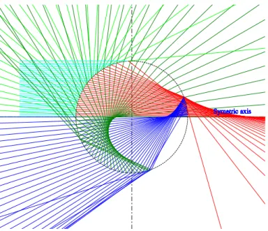
We present first in Fig. 2.7 the ray tracing in and out of a sphere. For clarity, only the above half of the sphere is illuminated (in cyan color). The reflected rays (p = 0 in green) spread in all directions. The refracted rays (p = 1 in red) are confined in the forward directions and experience a focal point outside of the particle (passing by the symmetric axis) and the rays far from the axis may have a focal line inside the particle. The rays of second order p = 2 (in blue) and third order p = 3 (in dark green) have each of them a extreme deviation angle, about 138◦ for p = 2 and 127◦ for p = 3, where the scattered intensity predicted by GO tends to infinity. These are the so called geometrical rainbow angles.

Then the intensity of the emergent rays of different orders as well as the total scattered intensity calculated by GO are shown in Fig. 2.8. The minimum value of the order of

(43)

Symetric axis Symetric axis Symetric axis Symetric axis Symetric axis Symetric axis Symetric axis Symetric axis Symetric axis Symetric axis Symetric axis Symetric axis Symetric axis Symetric axis Symetric axis Symetric axis Symetric axis Symetric axis Symetric axis Symetric axis Symetric axis Symetric axis Symetric axis Symetric axis Symetric axis Symetric axis Symetric axis Symetric axis Symetric axis Symetric axis

Figure 2.7: Ray tracing by GO for a sphere (m = 1.333) illuminated by a plane wave. For clarity, only the above half of the sphere is considered with p = 3.

ray is 0 and the maximum value of that is 4. The interference is taken into account for the total intensity but not for the individual orders. The intensity of the individual order is determined by the two factors: the Fresnel coefficients and the divergence factor. For example, the intensity of the rays of order p = 0 decreases monotonically as function of scattering angle for the perpendicular polarization but tends to zero at 74◦ for the parallel polarization the later corresponds to the Brewster angle θB = 53.12◦

because the scattering angle is related to the incident angle by θs = 2τ = 2(90◦− θi)

for p = 0. Similarly, the minimum intensity for the parallel polarization in the other orders are all due to the Brewster angle.

At the same time we observe that all the peaks are located at the same angles for the two polarization. These are due to the divergence factor, which are independent of the polarization and can be predicted by the formulas given in the previous section.

To evaluate the accuracy of the GO, we will compare the scattered intensities calculated by the GO and the LMT for a particle of radius illuminated by a plane wave. For a complete comparison, the diffraction must be taken into account. This can be done by considering the sphere as a opaque disk of the same section. The amplitude of the diffracted field is given by

Ad(θ) = α

J1(αθ)

αθ (2.39)

where, J1 is the first-order Bessel function of the first kind. Ad(θ) is added into Eq.

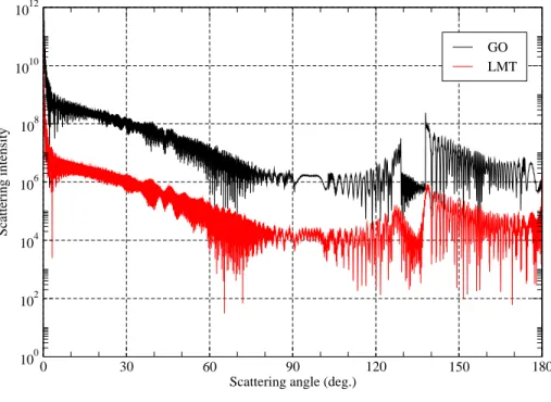
(2.37) The scattered diagrams calculated by the two methods for a particle of a large particle (a = 100 µm, m = 1.333) are given in Fig. 2.9. The minimum value of the order of ray is 0 and the maximum value of that is 12 in scattered intensity with GO. We find that the agreement is very satisfactory in general. However, a discrepancy

(44)

0 30 60 90 120 150 180 Scattering angle (deg.)

10-2 100 102 104 106 108 Scattering intensity p = 0 p = 1 p = 2 p = 3 p = 4 total

(a) Perpendicular polarization

0 30 60 90 120 150 180

Scattering angle (deg.)

10-6 10-4 10-2 100 102 104 106 108 Scattering Intensity p = 0 p = 1 p = 2 p = 3 p = 4 total (b) Parallel polarization

Figure 2.8: Scattered intensity of each order of rays and the total intensity (plane wave