HAL Id: hal-01121110
https://hal.inria.fr/hal-01121110
Submitted on 27 Feb 2015
HAL is a multi-disciplinary open access
archive for the deposit and dissemination of
sci-entific research documents, whether they are
pub-lished or not. The documents may come from
teaching and research institutions in France or
abroad, or from public or private research centers.
L’archive ouverte pluridisciplinaire HAL, est
destinée au dépôt et à la diffusion de documents
scientifiques de niveau recherche, publiés ou non,
émanant des établissements d’enseignement et de
recherche français ou étrangers, des laboratoires
publics ou privés.
Hrishikesh Deshpande, Pierre Maurel, Christian Barillot
To cite this version:
Hrishikesh Deshpande, Pierre Maurel, Christian Barillot. Adaptive Dictionary Learning For
Com-petitive Classification Of Multiple Sclerosis Lesions. International Symposium on BIOMEDICAL
IMAGING: From Nano to Macro, Apr 2015, New-York, United States. �hal-01121110�
ADAPTIVE DICTIONARY LEARNING FOR COMPETITIVE CLASSIFICATION OF
MULTIPLE SCLEROSIS LESIONS
Hrishikesh Deshpande, Pierre Maurel, Christian Barillot
Inria, VisAGeS INSERM U746, IRISA UMR CNRS 6074, University of Rennes-1, Rennes, France
ABSTRACT
Sparse representations allow modeling data using a few basis elements of an over-complete dictionary and have been used in many image processing applications. We propose to use a sparse representation and an adaptive dictionary learning paradigm to automatically classify Multiple Sclerosis (MS) lesions from MRI. In particular, we investigate the effects of learning dictionaries specific to the lesions and individ-ual healthy brain tissues, which include White Matter (WM), Gray Matter (GM) and Cerebrospinal Fluid (CSF). The dic-tionary size plays a major role in data representation but it is an even more crucial element in the case of competitive classification. We present an approach that adapts the size of the dictionary for each class, depending on the complexity of the underlying data. The proposed algorithm is evaluated on clinical data demonstrating improved classification.
Index Terms— Sparse Representations, Adaptive Dictio-nary Learning, Magnetic Resonance Imaging
1. INTRODUCTION
An important variety of natural images can be represented as linear combinations of a few atoms of a learned dictio-nary. Over the last few years, researchers have shown that the sparse representation of the images in such a way produces promising results in image denoising and classification, in-cluding face recognition and texture classification [1–3]. Re-cently, its applications in disease detection have started evolv-ing [4, 5]. In this paper, we present a novel method usevolv-ing sparse representations and dictionary learning framework to classify MS lesions.
Multiple sclerosis is an autoimmune disease affecting the central nervous system and is characterized by the structural damages of axons. MRI is the best paraclinical method for the diagnosis of MS and treatment efficacy. Manual segmentation of MS lesions, however, is a laborious and time consuming task, and is prone to high intra- and inter-expert variability. Several MS lesion segmentation methods have been proposed over the last decades, with an objective of handling large va-riety of MR data and which can provide results that correlate well with expert analysis [6]. These methods either use lesion properties or tissue segmentation to help lesion segmentation.
We investigate the performance of automatic lesion clas-sification by taking into account the tissue specific informa-tion. In the past, Weiss et al. [4] treated lesions as outliers and achieved MS lesion segmentation using a single dictio-nary learned with the help of all image patches. Deshpande et al.[5] reported improvements by learning class specific dic-tionaries for the lesion and healthy tissue patches. However, we can further enrich this model by using dictionaries spe-cific to the different tissue types, such as WM, GM and CSF, as opposed to learning a single dictionary for healthy tissue patches. We explore the fact that various tissues as well as lesions appear in different intensity patterns in distinct MR modality images. For example, WM appears as the brightest tissue in T1-weighted image, but the darkest in T2-weighted images. Therefore, learning class specific dictionaries for in-dividual tissues should further discriminate between lesion and non-lesion classes. We consider multiple MR modality images and learn the tissue specific dictionaries for WM, GM, CSF and lesion classes, to better classify MS lesions.
The dictionaries learned for each class are aimed at bet-ter representation of an individual class. However, if there exists differences in the data-complexity between classes, the relative under- or over-representation of either class will lead to worse classification. One idea for better classification could be to learn the dictionaries with adaptive sizes, in order to take into account the data variability between different classes. Thus, in addition to the dictionary learning strategy mentioned above, we also investigate the effect of modifying the dictionary sizes, leading to the proposition of adaptive dictionary learning. The basic idea is to learn the class spe-cific dictionaries which are better adapted to the data and also complexity of the data. Previous works [5, 7] have also reported the effects of dictionary size in image classification. We investigate this in the particular case of classification.
We first describe sparse coding and dictionary learning in Section 2. The methodology is explained in Section 3, fol-lowed by results in Section 4 and conclusion in Section 5.
2. SPARSE CODING AND DICTIONARY LEARNING Sparse coding is the process of finding a sparse coefficient vector a ∈ RKfor representing a given signal x ∈ RN using a few atoms of an over-complete dictionary D ∈ RN ×K. It is
given by minakak0s.t. kx − Dak 2
2≤ ε, where k.k0denotes
the l0norm and ε is the error in representation. Replacement
of l0norm with the l1norm also results in sparse solution [8].
The sparse coding problem can then be given by min
a kx − Dak 2
2+ λ kak1, (1)
where λ balances the trade-off between the error and sparsity. For a set of signals {xi}i=1,.,m, we can find a dictionary D
from the underlying data, such that each signal is represented by a sparse linear combination of its atoms. It is given by
min D,{ai}i=1,..,m m X i=1 kxi− Daik 2 2+ λ kaik1. (2)
The optimization is an iterative two-step process: Sparse cod-ing with fixed D and the dictionary update with fixed a.
3. PROPOSED APPROACH
MR images from each patient are first processed for the re-moval of noise and non-brain tissues. The images are then registered and image patches of predefined size are extracted. These patches, after intensity normalization, are assigned to WM, GM, CSF or lesion class. For this purpose, we use man-ual lesion segmentation images and tissue segmentation ob-tained using SPM [9]. We then learn the dictionaries using training data for each class and perform patch based classifi-cation and voxel-wise classificlassifi-cation for the given test subject. Each step is described in the subsections below.
3.1. Pre-processing
The noise introduced during MR acquisition is removed using non-local means and intensity inhomogenity correction [10, 11]. To ensure the spatial correspondence, the images are reg-istered with respect to T1-w MPRAGE volume [12] and are processed further to extract the intra-cranial mask [13]. This limits the further analysis to the brain region.
3.2. Patch Extraction and Labeling
We divide the whole intracranial MR volume for each patient into 3-D patches, with a patch around every 2 voxels in each direction. The individual image patches of each MR modality are then flattened, concatenated together and are normalized. The patches are then labelled as either WM, GM, CSF or le-sion class. If the number of lele-sion voxels in the corresponding image block of the manual segmentation image exceeds the pre-defined threshold TL, we assign this patch to the lesion
class. Otherwise, the patch is assigned to either WM, GM or CSF class, depending on the maximum number of voxels that belong to the corresponding class.
The labelled image patches are then divided into training and test data, and the experiments are performed by following Leave-One-Subject-Out-Cross-Validation (LOSOCV).
3.3. Classification using Adaptive Dictionary Learning The class specific dictionaries are learned using training data of the corresponding class [14]. The subsections below de-scribe different strategies adopted while learning these dictio-naries and the scheme of patch based classification. In every method, we obtain the sparse codes for the test patches using Eq (1), knowing the dictionary Dkfor the class k [14].
3.3.1. Two-Class: Same Dictionary Size (2-C SDS)
Similar to [5], we use a single dictionary to represent the healthy class: WM, GM and CSF together. We learn the class specific dictionaries Dkof same size, for the healthy (k = 1) and lesion (k = 2) class. For a given test patch yi, the
clas-sification is performed by calculating the sparse coefficients aki for each class and the test patch is then assigned to class c such that c = argmin k yi− Dkaki 2 2. (3)
3.3.2. Two-Class: Different Dictionary Size (2-C DDS) In this method, we allow different dictionary sizes for the healthy and lesion classes, in order to take into consideration the data variability between classes and the number of train-ing samples in each class. For accounttrain-ing to more variability and larger training size, we allow larger dictionary size for the healthy class and obtain MS lesion classification.
3.3.3. Four-Class: Same Dictionary Size (4-C SDS)
The fact that every tissue, WM, GM and CSF, appears in dif-ferent intensity pattern in each MR modality, using a single dictionary for representing tissues might not be as effective as learning separate dictionaries for each tissue. Each dictionary is representative of its own class and reconstruction of the test data using true class dictionary would give the minimum re-construction error. We thus perform classification based on reconstruction error in a similar manner, as mentioned above. 3.3.4. Four-Class: Different Dictionary Size (4-C DDS) Here, we experiment with different dictionary sizes for WM, GM, CSF and lesion classes, for similar reasons mentioned in Section 3.3.2.
3.4. Voxel-wise Classification
As already stated, we classify the patches centered around ev-ery 2 voxels in each direction. For voxel-wise classification, we assign each voxel to either of the classes by using majority voting. The voxel is assigned to a class using majority votes of all patches that contain the voxel.
In the context of lesion classification, we finally record the number of voxels that belong to True Positives (TP), False
Negatives (FN) or False Positives (FP), and calculate sensi-tivity (SEN)= T P +F NT P and Positive Predictive Value (PPV)
= T P
T P +F P.
4. EXPERIMENTS AND RESULTS
We evaluated the proposed approach on MR dataset of 14 MS patients acquired on a Verio 3T Siemens scanner. T1-w MPRAGE, T2-w, PD and FLAIR modalities were chosen for the analysis. The volume size for T1-w MPRAGE and FLAIR was 256×256×160 and voxel size was 1×1×1 mm3. For T2-w and PD, the volume size T2-was 256×256×44 and voxel size was 1×1×3 mm3. Annotations of the lesions were carried out by an expert radiologist. One subject with strong MR artifacts was excluded from the analysis.
For labeling patches, we used threshold TL= 6, as
men-tioned in Section 3.2. For each subject, the number of lesion patches varied from 1K to 30K, depending on the lesion load, whereas the average number of patches for WM, GM and CSF were 50K, 90K and 30K respectively. Using LOSOCV, the patch size of 5×5×5 and the sparsity parameter λ = 0.95 were found to be optimal choices. We used these parameters for all experiments described next.
The voxel-wise classification results for the methods de-scribed above are shown in Table 1. Using same dictionary size of 5000 for healthy and lesion class, as denoted by method (a), results in high sensitivity but very low PPV. Con-sidering more variability associated with the healthy class, we then use different dictionary sizes, 5000 for healthy and 1000 for lesion class. This drastically reduces FP, improving PPV, but also decreases sensitivity. We further enrich this model by learning tissue specific dictionaries for WM, GM, CSF. Using 4-class approach and the same dictionary size of 2000 for each tissue and lesion class gives better compromise between sensitivity and PPV. Finally, 4-class method with different dictionary sizes, 2000 each for WM, GM and CSF, and 1000 for lesion class, increases both the mean sensitivity and PPV values, as compared to the 2-class method with different dictionary sizes. The mean dice-scores for methods (b) and (d), as referred to in Table 1, are 43.46% and 48.20%, respectively. Their comparison also shows a significant dif-ference in PPV and dice-scores, with respective p-values of 0.0086 and 0.0298. This confirms that learning class specific dictionaries for each tissue improves the classification.
The classification performance for various dictionary sizes in the 4-class methods is shown in Table 2. The results for method (c), in row X, show that the sensitivity and PPV increase until the dictionary sizes are increased to 2000. The dictionaries capture more details with the increase in their size, but sensitivity reduces thereafter, possibly because of the over-fitting in either class dictionary. In rows Y and Z, we fix the size of either lesion or tissue dictionaries and vary the size of the other. It is observed that the best results, in terms of both sensitivity and PPV, are obtained for the dictionary
Pat. (a) (b) (c) (d)
No. 2-C SDS 2-C DDS 4-C SDS 4-C DDS
SEN PPV SEN PPV SEN PPV SEN PPV
1 97 3 53 31 68 11 32 34 2 98 2 66 41 78 9 60 38 3 91 2 63 27 72 9 58 31 4 98 17 57 68 89 50 69 83 5 95 10 54 65 85 43 68 71 6 89 29 38 55 80 48 56 64 7 85 3 20 32 68 20 38 34 8 98 3 69 21 89 10 72 24 9 97 9 61 52 84 33 68 62 10 98 12 66 41 91 29 73 47 11 99 8 52 36 82 20 58 39 12 100 3 77 31 91 11 72 30 13 100 2 78 17 90 5 68 16 Avg 95.8 7.9 58 39.8 82.1 22.9 60.9 44.1
Table 1. Voxel-wise classification results using: (a) Two dic-tionaries with 5000 atoms for healthy and lesion classes (b) 5000 atoms for healthy and 1000 atoms for lesion class dic-tionary. (c) Four dictionaries with 2000 atoms for WM, GM, CSF and lesion class, (d) 2000 atoms for WM, GM and CSF, and 1000 atoms for lesion class dictionary.
size of 2000 for each tissue and 1000 for lesion class. It can also be observed that it is the relative dictionary size that drives the classification and is more important than just the absolute dictionary size for each class.
It is crucial to adapt the size of the dictionaries to better control the classification. For such purpose, we analyzed the data using Principal Component Analysis (PCA), which gives an estimate of the intrinsic dimensionality of the data. It was found that for each tissue, GM, WM and CSF, approximately twice as many eigenvalues are required for an arbitrary pro-portion of the cumulative data variance (90%, 95% or 98%), as that required for the lesion data. Thus, as exhibited by method (d), it supports our adaption of the dictionary size for each tissue twice that for the lesion dictionary. For method (b), although the experimentally observed optimal dictionary size ratio of 5 was not found with PCA, the factor of 2 in-dicated by PCA still favors using higher dictionary size for the healthy class. One reasoning behind this might be the in-ability of PCA to analyze the non-linearity in the data. The intrinsic dimensionality estimation for this highly non-linear data could be further point of investigation.
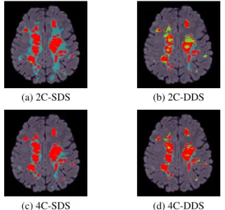
In Figure 1, we show the results for patient 6, for all the methods discussed above. It can be seen that the methods (a) and (c), each using the dictionaries with the same size, suffer with many FP. The over-detections are reduced in methods (b) and (d), respectively, which use the adapted dictionary sizes. However, the 2-class method (b) has many FN. Including tis-sue specific information in the approach and using dictionar-ies of the adapted sizes results in significant improvement in the lesion classification with reduction in both FP and FN. This is shown in method (d), supporting our claim that the
Tissues Lesion SEN PPV X 500 500 81.1 17.2 1000 1000 81.8 19.7 2000 2000 82.1 22.9 5000 5000 80.6 25.5 Y 500 1000 94.9 5.2 2000 1000 60.9 44.1 5000 1000 30 67.5 Z 2000 500 32.7 65.1 2000 1000 60.9 44.1 2000 5000 95.3 6.5
Table 2. Effect of dictionary sizes in classification. First two columns indicate the dictionary size for each tissue and lesion, whereas the last two columns indicate the sensitivity and PPV. Row X: Method (c) with various dictionary sizes, Rows Y and Z: Method (d) with fixed dictionary size for either lesion or tissues, while varying dictionary sizes for the other class.
method with the tissue specific dictionaries and adapted dic-tionary sizes is a better choice over the 2-class methods and those using the same dictionary size.
(a) 2C-SDS (b) 2C-DDS
(c) 4C-SDS (d) 4C-DDS
Fig. 1. Comparison of MS lesion classification methods, as referred in Table 1. Classification image is superimposed on FLAIR MRI. TP are in red, FP are in cyan, FN are in green.
5. CONCLUSION
An approach for MS lesion classification based on dictionary learning and sparse representations is introduced in this work. Learning tissue specific dictionaries, instead of using a single dictionary for the non-lesion class, has shown clear improve-ment in the lesion classification. We have also demonstrated the effectiveness of adapting the dictionary sizes for better amplification of the differences among classes, hence
improv-ing the classification. If performimprov-ing PCA on input data can successfully adapt the dictionary size for the classification, it is not as much efficient when the classes represent more a mixture of different tissues. Knowing the limitation of PCA to handle only linear data, a future work will be to use the intrinsic dimension estimation techniques, which can better analyze complexity of the non-linear data.
6. REFERENCES
[1] M. Elad and M. Aharon, “Image denoising via learned dictionaries and sparse representation,” in CVPR, June 2006, vol. 1, pp. 895–900.
[2] J. Wright, A. Yang, et al., “Robust face recognition via sparse representation,” IEEE Trans. on PAMI, vol. 31, no. 2, pp. 210–227, Feb 2009.
[3] J. Mairal, J. Ponce, et al., “Supervised dictionary learn-ing,” in NIPS, pp. 1033–1040. 2009.
[4] N. Weiss et al., “Multiple sclerosis lesion segmentation using dictionary learning and sparse coding,” in MIC-CAI 2013, vol. 8149, pp. 735–742. 2013.
[5] H. Deshpande et al., “Detection of multiple sclerosis le-sions using sparse representations and dictionary learn-ing,” in MICCAI STMI Workshop, pp. 71–79. 2014. [6] X. Llad´o et al., “Segmentation of multiple sclerosis
le-sions in brain MRI: A review of automated approaches,” Information Sci., vol. 186, no. 1, pp. 164 – 185, 2012. [7] I. Ramirez and G. Sapiro, “An MDL framework for
sparse coding and dictionary learning,” IEEE Trans. on SP, vol. 60, no. 6, pp. 2913–2927, June 2012.
[8] S. Chen, D. Donoho, et al., “Atomic decomposition by basis pursuit,” SISC, vol. 20, pp. 33–61, 1998.
[9] J. Ashburner and K. Friston, “Unified segmentation,” NeuroImage, vol. 26, no. 3, pp. 839 – 851, 2005. [10] N. Tustison, B. Avants, et al., “N4ITK: Improved N3
bias correction,” IEEE TMI, vol. 29, no. 6, pp. 1310– 1320, June 2010.
[11] P. Coupe et al., “Optimized blockwise nonlocal means denoising filter for 3-D magnetic resonance images,” IEEE TMI, vol. 27, no. 4, pp. 425–441, April 2008. [12] W. Wells III, P. Viola, et al., “Multi-modal volume
reg-istration by maximization of mutual information,” Med-ical Image Analysis, vol. 1, no. 1, pp. 35 – 51, 1996. [13] S. Smith, “Fast robust automated brain extraction,”
Hu-man Brain Mapping, vol. 17, no. 3, pp. 143–155, 2002. [14] J. Mairal, F. Bach, et al., “Online dictionary learning for