HAL Id: hal-01497501
https://hal.archives-ouvertes.fr/hal-01497501
Submitted on 27 Oct 2020
HAL is a multi-disciplinary open access
archive for the deposit and dissemination of
sci-entific research documents, whether they are
pub-lished or not. The documents may come from
teaching and research institutions in France or
abroad, or from public or private research centers.
L’archive ouverte pluridisciplinaire HAL, est
destinée au dépôt et à la diffusion de documents
scientifiques de niveau recherche, publiés ou non,
émanant des établissements d’enseignement et de
recherche français ou étrangers, des laboratoires
publics ou privés.
Coastal-ocean uptake of anthropogenic carbon
Timothée Bourgeois, James C. Orr, Laure Resplandy, Jens Terhaar, Christian
Éthé, Marion Gehlen, Laurent Bopp
To cite this version:
Timothée Bourgeois, James C. Orr, Laure Resplandy, Jens Terhaar, Christian Éthé, et al..
Coastal-ocean uptake of anthropogenic carbon. Biogeosciences, European Geosciences Union, 2016, 13 (14),
pp.4167 - 4185. �10.5194/bg-13-4167-2016�. �hal-01497501�
www.biogeosciences.net/13/4167/2016/ doi:10.5194/bg-13-4167-2016
© Author(s) 2016. CC Attribution 3.0 License.
Coastal-ocean uptake of anthropogenic carbon
Timothée Bourgeois1, James C. Orr1, Laure Resplandy2, Jens Terhaar1, Christian Ethé3, Marion Gehlen1, and
Laurent Bopp1
1Laboratoire des Sciences du Climat et de l’Environnement, LSCE/IPSL, CEA-CNRS-UVSQ, Université Paris-Saclay,
91191 Gif-sur-Yvette, France
2Scripps Institution of Oceanography, University of California San Diego, La Jolla, CA, USA 3Institut Pierre Simon Laplace, 4 Place Jussieu, 75005 Paris, France
Correspondence to:Timothée Bourgeois (timothee.bourgeois@lsce.ipsl.fr)
Received: 18 February 2016 – Published in Biogeosciences Discuss.: 22 February 2016 Revised: 15 June 2016 – Accepted: 17 June 2016 – Published: 22 July 2016
Abstract. Anthropogenic changes in atmosphere–ocean and atmosphere–land CO2 fluxes have been quantified
exten-sively, but few studies have addressed the connection be-tween land and ocean. In this transition zone, the coastal ocean, spatial and temporal data coverage is inadequate to assess its global budget. Thus we use a global ocean biogeo-chemical model to assess the coastal ocean’s global inven-tory of anthropogenic CO2and its spatial variability. We used
an intermediate resolution, eddying version of the NEMO-PISCES model (ORCA05), varying from 20 to 50 km hor-izontally, i.e. coarse enough to allow multiple century-scale simulations but finer than coarse-resolution models (∼ 200 km) to better resolve coastal bathymetry and complex coastal currents. Here we define the coastal zone as the con-tinental shelf area, excluding the proximal zone. Evaluation of the simulated air–sea fluxes of total CO2for 45 coastal
re-gions gave a correlation coefficient R of 0.8 when compared to observation-based estimates. Simulated global uptake of anthropogenic carbon results averaged 2.3 Pg C yr−1 during the years 1993–2012, consistent with previous estimates. Yet only 0.1 Pg C yr−1 of that is absorbed by the global coastal ocean. That represents 4.5 % of the anthropogenic carbon uptake of the global ocean, less than the 7.5 % proportion of coastal-to-global-ocean surface areas. Coastal uptake is weakened due to a bottleneck in offshore transport, which is inadequate to reduce the mean anthropogenic carbon con-centration of coastal waters to the mean level found in the open-ocean mixed layer.
1 Introduction
The ocean mitigates climate change by absorbing atmo-spheric CO2 produced by combustion of fossil fuels,
land-use change, and cement production. During the 2005–2014 period, the global ocean absorbed 2.6 ± 0.5 Pg C yr−1of an-thropogenic carbon, an estimated 26 % of the total anthro-pogenic CO2 emissions (Le Quéré et al., 2015). The global
anthropogenic carbon budget relies on separate estimates for atmosphere, land, and ocean reservoirs. Yet it neglects what happens in the aquatic continuum between land and ocean (Cai, 2011; Regnier et al., 2013), for which there is no con-sensus on anthropogenic carbon uptake (Wanninkhof et al., 2013; Mackenzie et al., 2004; Bauer et al., 2013; Regnier et al., 2013; Le Quéré et al., 2015; Ciais et al., 2013).
The land–ocean aquatic continuum includes inland waters, estuaries, and the coastal ocean, i.e. the succession of active physical–biogeochemical systems that connect upland terres-trial soils to the open ocean (Regnier et al., 2013). Our fo-cus here is on the coastal ocean, which plays an inordinately large role relative to the open ocean in terms of primary pro-ductivity, export production, and carbon burial. Although the coastal ocean covers only 7–10 % of the global ocean sur-face area, it accounts for up to 30 % of oceanic primary pro-duction, 30–50 % of oceanic inorganic carbon burial, and 80 % of oceanic organic carbon burial (Gattuso et al., 1998; Longhurst et al., 1995; Walsh, 1991); moreover, the coastal-ocean supplies about half of the organic carbon that is deliv-ered to the deep open ocean (Liu et al., 2010). All these esti-mates suffer from high uncertainties as do those for coastal-ocean air–sea CO2exchange (Laruelle et al., 2014),
particu-2
larly its anthropogenic component. Indeed, in addition to the effect of increasing atmospheric CO2, potential changes in
coastal-ocean physics (e.g. temperature) and biology (e.g. net ecosystem production) as well as changes in riverine input, and interactions with the sediment may be of primary im-portance (Mackenzie et al., 2004; Hu and Cai, 2011). These changes would modify the distribution of carbon and alkalin-ity, hence change the potential of the coastal ocean to absorb anthropogenic carbon.
To date, few studies have distinguished anthropogenic car-bon uptake by the global coastal ocean. Estimating air–sea fluxes of anthropogenic CO2in the coastal ocean would
re-quire multi-decadal time series of coastal CO2observations
in order to extract an anthropogenic signal from the strong coastal natural variability. Such time series are still rare and probably not long enough. To our knowledge, the only avail-able equivalent time series are the Ishii et al. (2011) 1994– 2008 time series along 137◦E on Japanese coasts and the
Astor et al. (2013) 1996–2008 time series at the CARIACO station on Venezuelan coasts. Therefore, estimates of anthro-pogenic carbon uptake by the global coastal ocean have been based on modelling studies, extrapolating data and model output from the open-ocean, and estimating residuals with budget calculations. An early modelling approach was pro-posed by Andersson and Mackenzie (2004) and Mackenzie et al. (2004). They used a 2-box model (Shallow-water Ocean Carbonate Model, SOCM) that separated the coastal ocean into surface waters and sediment pore waters. They estimated that the preindustrial coastal ocean was a source of CO2to
the atmosphere and had recently switched to a CO2 sink.
This source-to-sink switch is mainly caused by a shift in net ecosystem production (NEP) due to increased anthropogenic nutrient inputs (Andersson and Mackenzie, 2004; Mackenzie et al., 2004). Another proposed mechanism is simply linked to the anthropogenic increase in atmospheric CO2,
consider-ing constant NEP (Bauer et al., 2013). The difference
be-tween the simulated air–sea CO2 fluxes from the SOCM
model for the years 1700 and 2000 suggests that in 2000 the coastal ocean absorbed 0.17 Pg C yr−1of anthropogenic car-bon from the atmosphere (Borges, 2005). As for extrapola-tion, Wanninkhof et al. (2013) used coarse-resolution global-ocean models and observations and estimated a similar up-take of 0.18 Pg C yr−1 by extrapolating open-ocean air–sea fluxes of anthropogenic CO2into the coastal zone. Finally,
Liu et al. (2010) combined estimates from the same SOCM model for the preindustrial coastal zone with observational estimates of the contemporary flux to deduce a corresponding anthropogenic carbon uptake of 0.5 Pg C yr−1for the 1990s.
In addition, there exist 3-D regional-circulation–
biogeochemistry–ecosystem models that have been used to study other aspects of coastal-ocean carbon cycling as sum-marized by Hofmann et al. (2011). Typically, such models have been implemented in regions where sufficient measure-ments are available for model validation, e.g. the Middle Atlantic Bight (eastern US coast) (Fennel et al., 2008;
Fennel, 2010), the California current system (Fiechter et al., 2014; Turi et al., 2014; Lachkar and Gruber, 2013), and the European shelf seas (Artioli et al., 2014; Phelps et al., 2014; Wakelin et al., 2012; Allen et al., 2001; Cossarini et al., 2015; Prowe et al., 2009). Because of their limited regional domains, such models are typically able to make simulations with horizontal resolutions of 10 km or less, which remains a challenge for global-circulation–biogeochemical models. The reduced computational requirements of regional models also allow biogeochemistry and ecosystem components to be more complex. Unfortunately, joining together a network of regional models to allow efficient simulations that cover all parts of the global coastal ocean remains a technical challenge (Holt et al., 2009).
The alternative to using a global model is computa-tionally more challenging because few of them have ade-quate resolution to properly simulate many critical coastal-ocean processes (Griffies et al., 2010; Holt et al., 2009). Coarse-resolution global models fail to adequately resolve the coastal bathymetry, which substantially alters coastal-ocean circulation (Fiechter et al., 2014) as well as mesoscale dynamics, upwelling, and coastal currents, all of which are thought to strongly affect the variability of air–sea CO2
fluxes along ocean margins (Borges, 2005; Lachkar et al., 2007; Kelley et al., 1971). Global models also typically lack a benthic component, i.e. early diagenesis in sediments, which in some regions is likely to affect simulated coastal-ocean biogeochemistry of overlying waters. Moreover, input of car-bon and nutrients from rivers and groundwater is usually lacking. Even in models such as ours, where that input is imposed as boundary conditions (Aumont et al., 2015), tem-poral variability and trends are neglected (Bauer et al., 2013; Cotrim da Cunha et al., 2007).
Nonetheless, coarse-resolution models are no longer state of the art. Recently, there have been improvements in spatial resolution of global ocean models and the spatio-temporal resolution of surface forcing fields (Brodeau et al., 2010), thereby improving the representation of bathymetry and ocean processes in the highly variable coastal zone (Capet, 2004; Hofmann et al., 2011; McKiver et al., 2014). In any case, models currently provide the only means to estimate coastal uptake of anthropogenic carbon due to the lack of data-based estimates.
Here our aim is to estimate the air-to-sea flux of anthro-pogenic CO2into the coastal ocean and how it varies from
region to region across the globe. We focus solely on the geochemical effect of anthropogenic CO2addition from the
atmosphere to the ocean and neglect the role of varying river input and interactions with the sediment, as well as feedback from a changing climate. To do so, we rely on an eddying ver-sion of the global NEMO circulation model (Madec, 2008), which also includes the LIM2 sea ice model and is coupled to the PISCES biogeochemical model (Aumont and Bopp, 2006). More precisely, we use the ORCA05 eddy-admitting resolution, which ranges from 0.2 to 0.5◦(i.e. 20 to 50 km).
Although this resolution does not fully resolve coastal-ocean bathymetry and dynamics, it does provide a first step into the eddying regime and a starting point upon which to compare future studies that will model the coastal ocean, globally, at higher resolution.
2 Methods
2.1 Coupled physical–biogeochemical model
For this study, we use version 3.2 of the ocean model known as NEMO (Nucleus for European Modelling of the Ocean), which includes (1) the primitive equation model Océan Parallélisé (OPA, Madec, 2008), (2) the dynamic-thermodynamic Louvain-La-Neuve sea ice model (LIM, Fichefet and Morales Maqueda, 1997), and (3) the Tracer in the Ocean Paradigm (TOP), a passive tracer module. Here the latter is connected to version 1 of the ocean biogeo-chemical model PISCES (Pelagic Interaction Scheme for Carbon and Ecosystem Studies) (Aumont and Bopp, 2006). For the NEMO model, we use a global-scale configuration from the DRAKKAR community (see Barnier et al., 2006; Timmermann et al., 2005). Namely, we use the ORCA05 global configuration, which possesses a curvilinear, tripolar grid with a horizontal resolution that ranges between 0.2◦ near the North Pole to 0.5◦ at the Equator (Fig. 1). Verti-cally, ORCA05 is discretized into 46 levels with thicknesses that range from 6 m at the surface to 250 m for the deepest ocean level (centred at 5625 m). Model bathymetry is com-puted from the 2 min bathymetry file ETOPO2 from the Na-tional Geophysical Data Center. The numerical characteris-tics of our ORCA05 configuration follow the lead of Barnier et al. (2006) for the ORCA025 configuration with resolution-dependent modifications for the horizontal eddy diffusivity for tracers modified to 600 m2s−1and horizontal eddy vis-cosity fixed to −4 × 10¹¹m2s−1. To simulate the advective transport driven by geostrophic eddies, our ORCA05 simu-lation uses the eddy parameterization scheme of Gent and McWilliams (1990) applied with an eddy diffusion coeffi-cient of 1000 m2s−1.
The biogeochemical model PISCES includes four plank-ton functional types: two phytoplankplank-ton (nanophytoplank-ton and diatoms) and two zooplank(nanophytoplank-ton (micro- and mesozoo-plankton). PISCES also uses a mixed-quota Monod approach where (1) phytoplankton growth is limited by five nutrients (nitrate, ammonium, phosphate iron, and silicate), following Monod (1949) and (2) elemental ratios of Fe, Si, and Chl to C are prognostic variables based on the external concentrations of the limiting nutrients. In addition PISCES assumes a fixed C : N : P Redfield ratio set to 122 : 16 : 1 from Takahashi et al. (1985) for both living and non-living pools. Similar to Gei-der et al. (1998), the phytoplankton Chl:C ratio in PISCES varies with photoadaptation. Furthermore, PISCES includes non-living pools, namely a pool of semilabile dissolved
or-ganic matter and two size classes of particulate oror-ganic mat-ter. PISCES also explicitly accounts for biogenic silica and calcite particles. In PISCES, the sediment–water interface is treated as a reflective boundary condition where mass fluxes from particles are remineralized instantaneously, except that small proportions of particle fluxes of organic matter, calcite, and biogenic silica escape the system through burial. Those burial rates are hence dependent on the local sinking fluxes, but are set to balance inputs from rivers and atmospheric de-position at the global scale. Thus global budgets of alkalinity and nutrients are balanced. For further details, we refer read-ers to Aumont and Bopp (2006).
To simulate carbon chemistry and air–sea CO2 fluxes,
the model follows the protocol from phase 2 of the Ocean Carbon-Cycle Model Intercomparison Project (OCMIP, Na-jjar and Orr, 1999) protocol. The sea-to-air CO2flux FCO2is
computed using the following equation:
FCO2=α k 1pCO2, (1)
where α is the solubility of CO2 computed from Weiss
(1974) and 1pCO2is the difference between the partial
pres-sures of sea surface and atmospheric CO2. Thus FCO2is
pos-itive when CO2is transferred from the ocean to the
atmo-sphere. The piston velocity k is based on Eq. (3) of Wan-ninkhof (1992):
k =0.30 u2w r
660
Sc (1 − fice), (2)
where uwis the wind speed at 10 m, Sc is the CO2Schmidt
number, and ficeis the ice fraction.
2.2 Simulations
The dynamic model was started from rest and spun up for 50 years. Initial conditions for temperature and salinity are as described by Barnier et al. (2006). Initial biogeochemical fields of nitrate, phosphate, oxygen, and silicate are from the 2001 World Ocean Atlas (Conkright et al., 2002), whereas preindustrial dissolved inorganic carbon (DIC) and total al-kalinity (Alk) come from the GLODAP gridded product (Key et al., 2004). Conversely, because data for iron and dissolved organic carbon (DOC) are more limited, both those fields were initialized with model output from a 3000-year spin up simulation of a global 2◦configuration of the same NEMO-PISCES model (Aumont and Bopp, 2006). All other biogeo-chemical tracers have much shorter timescales; hence, they were initialized to globally uniform constants.
After the 50-year spin-up, we launched two parallel simu-lations: the first was a historical simulation run from 1870 to 2012 (143 years), and forced with a spatially uniform and temporally increasing atmospheric mole fraction of CO2
(from which PISCES computes atmospheric pCOatm2 follow-ing OCMIP2) reconstructed from ice core and atmospheric records (Le Quéré et al., 2014); the second simulation is a
2
Figure 1. (a) Global segmentation of the coastal ocean following Laruelle et al. (2013) as regridded on the ORCA05 model grid. Colours distinguish limits between the MARCATS regions, numbers indicate regions defined in LA13. To perceive the spatial resolution of the ORCA05 configuration in the MARCATS context, we show zoomed-in images of bathymetry in four regions: (b) the Arctic polar margins, (c) the North Sea, (d) the Sea of Japan, the China Sea, and Kuroshio, and (e) south-western Africa and the Agulhas current. In the latter three panels, grid resolution is indicated by thin black lines.
parallel control run, where the 143-year simulation is identi-cal except that it is forced with the preindustrial level of at-mospheric mole fraction of CO2(287 ppm, constant in time).
The preindustrial reference year is defined as 1870, thus neglecting changes in anthropogenic carbon storage in the ocean from 1750 to 1870. The FCO2 computed with the
his-torical simulation is for total carbon (total FCO2), whereas the
FCO2 from the control simulation is for natural carbon
(nat-ural FCO2). The corresponding anthropogenic FCO2 is
com-puted as the total minus natural FCO2.
All simulations were forced identically with atmospheric fields from the DRAKKAR Forcing Set (DFS, Brodeau et al., 2010). These fields include zonal and meridional compo-nents of 10 m winds, 2 m air humidity, 2 m air
tempera-ture, downward shortwave and longwave radiation at the sea surface, and precipitation. More specifically the NEMO-PISCES model is forced with version 4.2 of this forcing (DFS4.2, based on the ERA40 reanalysis) over 1958–2001, and that is followed by forcing from version 4.4 (DFS4.4) over 2002–2012. For the 1870–1957 period, where atmo-spheric reanalyses are unavailable, we repeatedly cycled the 1958–2007 DFS4.2 forcing.
Boundary conditions are also needed for biogeochemical tracers, i.e. besides the atmospheric CO2 connection
men-tioned already. The model’s lateral input from river discharge of DIC and DOC are taken from the annual estimates of the Global Erosion Model (Ludwig et al., 1996), constant in time. The DOC from river discharge is assumed to be la-bile and is directly converted to DIC upon its delivery to the ocean. Inputs of dissolved iron (Fe), nitrate (NO2−3 ), phos-phate (PO3−4 ), and silicate (SiO2) are computed from the sum
of DIC and DOC river input using a constant set of ratios for C : N : P : Si : Fe, namely 320 : 16 : 1 : 53.3 : 3.64 × 10⁻³, as computed from Meybeck (1982) for C : N, from Takahashi et al. (1985) for N : P, from de Baar and de Jong (2001) for Fe : C, and from Treguer et al. (1995) for Si : C. River dis-charge assumes no seasonal variation. Atmospheric deposi-tion of iron comes from Tegen and Fung (1995).
Here, we use the conventional definition of anthropogenic carbon in the ocean used by previous global-ocean model studies (OCMIP, http://ocmip5.ipsl.jussieu.fr/OCMIP/ and e.g. Bopp et al., 2015), namely that anthropogenic carbon comes only from the direct geochemical effect of increasing atmospheric CO2and its subsequent invasion into the ocean.
By definition, this anthropogenic FCO2 does not include any
effect from potential changes in ocean physics or biology. In the model, there are no changes nor variability in riverine de-livery of carbon and nutrients, and anthropogenic carbon is not buried in sediments.
Following the 50-year spin-up and 143-year control simu-lation, the simulation remains far from equilibrium. Its global natural carbon flux is −0.33 ± 0.3 Pg C yr−1(corresponding to CO2uptake by the ocean) during the last 10 years of the
control simulation (2003–2012), compared to the estimate of natural carbon outgassing of 0.45 Pg C yr−1by Jacobson et al. (2007). That difference is partly due to the strategy for our simulations, which were initialized with data and spun up for only 50 years because of the computational constraints to make higher-resolution simulations (ORCA05). At lower resolution (ORCA2), after a spin-up of 3000 years, there is 0.26 Pg C yr−1greater globally integrated sea-to-air flux, rel-ative to results after only a 50-year spin-up. Nearly all of that enhanced sea-to-air CO2flux due to the longer spin-up
comes from the Southern Ocean. Anthropogenic FCO2
esti-mates are expected to be influenced very little by model drift because of the way anthropogenic carbon is defined (i.e. drift affects both natural carbon and total carbon in the same way).
2.3 Defining the global coastal ocean
To sample the global coastal-ocean area, the model grid cells were selected following the MARgins and CATchments Seg-mentation (MARCATS) of Laruelle et al. (2013), hereafter LA13. The outer limit of the coastal ocean is defined as the maximum slope at the shelf break, while the inner limit is taken as the coastline, thus excluding the proximal zone of the coastal ocean (Fig. 1). Hence, only the continental shelf area is taken into account. The MARCATS segmentation di-vides the global coastal ocean into 45 regional units (Ta-ble 2). The limits of each of these units delineate areas that present roughly homogenous oceanic features such as coastal currents or the boundaries of marginal seas. Following the Liu et al. (2010) classification of the continental shelf seas, LA13 aggregated the 45 units into seven classes with similar physical and oceanographic large-scale characteristics such as the eastern boundary currents and the polar margins. The high-resolution geographical information system (GIS) file describing the MARCATS segmentation from LA13 was re-gridded using the QGIS software (QGIS Development Team, 2015) on the ORCA05 model grid in order to sample the model results on its own grid. This regridding technique im-plies some modifications to the regions initially described in LA13. In the model, the global coastal ocean has a total sur-face area of 27.0 × 10⁶km2, which is 8 % less than the origi-nal value from Laruelle et al. (2014). Here, the model’s total coastal-ocean surface area represents 7.5 % of the total area of the global ocean. Subsequently we refer to the individual MARCATS regions using the terminology of LA13.
2.4 Evaluation dataset
To evaluate the total FCO2 simulated by the model
(his-torical simulation), we compare it to the database from Laruelle et al. (2014), hereafter LA14, which provides observation-based estimates for the flux over the MAR-CATS regions. This database was constructed by aggregating 3 × 10⁶ coastal-sea surface pCO2 measurements collected
over 1990 to 2011 and included in the Surface Ocean CO2
Atlas version 2.0 (SOCAT v2.0, Pfeil et al., 2013; Bakker et al., 2014). These measurements represent about 30 % of the SOCAT v2.0 dataset. To compute the flux, LA14 also relied on wind speeds from the multiplatform CCMP wind speed database (Atlas et al., 2011), atmospheric CO2 from
GLOBALVIEW-CO2 (2012), and the flux parameterization from Wanninkhof (1992) as modified by Takahashi et al. (2009). As sensitivity tests, LA14 also used the flux parame-terizations from Ho et al. (2006) as well as the original for-mulation from Wanninkhof (1992).
Thus LA14 computed mean annual FCO2 estimates for 42
of the 45 MARCATS regions defined in LA13. The remain-ing MARCATS areas (12: Hudson Bay, 21: Black Sea and 29: Persian Gulf) are devoid of observations in the SOCAT database and were neglected. For the remaining regions,
be-2
cause of the large heterogeneity in both the spatial and tem-poral coverage of ocean pCO2observations, the
uncertain-ties for each of the MARCATS FCO2 estimates from LA14
vary greatly. For example, only 28 % of the sub-units of MARCATS regions used in LA14 have an estimate for FCO2
uncertainty of less than 0.25 mol C m−2yr−1. The data-based FCO2 estimate for the Sea of Okhotsk is not taken into
ac-count due to the extremely poor data coverage of this region and its strong divergence with the local literature (LA14). Here, we do not evaluate the simulated annual cycle of flux of total carbon because few MARCATS regions provide ad-equate temporal coverage. Finally, LA14 is the first and only study to provide coastal-ocean observation-based FCO2
es-timates at global scale taking into account the reduction in FCO2 due to sea ice cover along coasts; hence it is directly
comparable to our model results.
Besides the coastal data-based estimates of FCO2 from
LA14, we also compare our model results to those for the open ocean from Takahashi et al. (2009) and Landschützer et al. (2014). Both the global and coastal observational es-timates are compared to the average modelled FCO2 over
the last 20 years (1993–2012) of the historical simulation. For the coastal comparison, simulated total FCO2 are
spa-tially averaged over each MARCATS regions. In addition, the model’s uncertainty, computed as the interannual vari-ability over 1993–2012, is compared to uncertainties in the observational estimates, computed as the standard deviation between flux parameterizations from Wanninkhof (1992) as modified by Takahashi et al. (2009), Ho et al. (2006) and Wanninkhof (1992).
2.5 Revelle factor calculation
To assess how the capacity of the coastal ocean to absorb an-thropogenic carbon differs from open-ocean surface waters, we computed the Revelle factor (Rf, Sundquist et al., 1979)
using the CO2SYS MATLAB software (Van Heuven et al., 2011(@). CO2SYS was used with the simulated sea surface temperature, salinity, alkalinity, and DIC for model years 1993–2012 while choosing the total pH scale, the K1and K2
constants from Lueker et al. (2000), the KSO4 constant from
Dickson (1990), and the formulation of the borate-to-salinity ratio from Uppström (1974).
2.6 Residence time
To compute water residence time in each MARCATS region, we divided the volume of each region by the integrated out-flow of water from 5-day mean current velocities at coastal boundaries from 2011.
3 Results
3.1 Global ocean fluxes
The simulated global-ocean uptake of anthropogenic carbon increases roughly linearly from 1950 to 2012, reaching an av-erage of 2.3 Pg C yr−1during the period 1993–2012. That is comparable to the estimate from the fifth assessment report of the Intergovernmental Panel on Climate Change (IPCC) (Ciais et al., 2013) of 2.3 ± 0.7 Pg C yr−1 for 2000–2009 (Fig. 2).
Regionally, overall patterns in the total FCO2 are
simi-lar between the model and data-based estimates from Land-schützer et al. (2014) and Takahashi et al. (2009) (Fig. 3). Carbon is lost from the ocean in the equatorial band and in coastal upwelling regions, while it is gained by the ocean in the northern high latitudes. Quantitative comparison of the annual-mean map from the model with that from the Taka-hashi et al. (2009) observation-based database gives a root mean square error (RMSE) of 0.73 mol C m−2yr−1 and a correlation coefficient R of 0.80; likewise, comparison with the Landschützer et al. (2014) observational-based database gives a similar RMSE (0.70 mol C m−2yr−1) and R (0.81). Integrating over latitudinal bands, (Table 1), the model over-estimates carbon uptake for the 90–30◦S region, where it ab-sorbs 1.50 Pg C yr−1of total carbon vs. 0.73–0.77 Pg C yr−1 from Takahashi et al. (2009) and Landschützer et al. (2014) observational databases. This overestimate may result from the model simulation still being far from equilibrium (see Sect. 2.2 paragraph 5 for details). The model also under-estimates outgassing in the tropical band, where it releases 0.13 Pg C yr−1vs. 0.13–0.20 Pg C yr−1for the two data-based estimates. Further north in the 30–90◦N band, the model takes up 0.93 Pg C yr−1 vs. 1.53–1.59 Pg C yr−1 for Taka-hashi et al. (2009) and Landschützer et al. (2014).
3.2 Coastal-ocean fluxes
3.2.1 Total CO2
The simulated uptake of total carbon by the coastal-ocean averages 267 Tg C yr−1during the 1993–2012 period. Most of the 45 MARCATS regions act as carbon sinks; to-gether, they absorb 283 Tg C yr−1. The largest uptake is 3.4 mol C m−2yr−1 in the South Greenland region. Few MARCATS regions act as carbon sources to the atmosphere (Table 2 and Fig. 4.a), i.e. only 14 % of the global coastal-ocean surface area, together losing 16 Tg C of carbon to the atmosphere every year. The mean annual carbon loss per square metre in these MARCATS regions is usually rela-tively weak, less than 1.5 mol C m−2yr−1). When grouped into MARCATS classes (see Table 3), all classes are carbon sinks, absorbing from 0.06 to 1.65 mol C m−2yr−1. By class, the largest specific fluxes occur in the western boundary cur-rent regions and the subpolar margins, which absorb 1.65
Figure 2. Simulated temporal evolution of area-integrated anthropogenic carbon uptake for (a) the open ocean and (b) the coastal ocean. (c) Analogous evolution of anthropogenic carbon uptake for the open ocean, the coastal ocean, the Southern Ocean, and the tropical oceans, but given as the average flux per unit area.
Table 1. Sea-to-air total CO2 fluxes (Pg C yr−1) given as zonal means from Takahashi et al. (2009) for the reference year 2000, from
Landschützer et al. (2014) for 1998–2011 and the ORCA05 model for 1993–2012.
Latitudinal Observation-based climatologies This study
bands Takahashi et al. (2009) Landschützer et al. (2014) ORCA05
90–30◦S −0.77 −0.73 −1.50
30◦S–30◦N 0.20 0.13 0.13
30–90◦N −1.59 −1.53 −0.93
and 1.61 mol C m−2yr−1 respectively. More generally, the tropical MARCATS regions act as weak carbon sources and the mid-to-high-latitude regions act as strong carbon sinks (Fig. 4a). The same trend is also apparent in the zonal-mean distribution (Fig. 5).
A comparison of the simulated vs. observed FCO2
esti-mates for each MARCATS region is reported in Table 2 and Fig. 6. The Pearson correlation coefficient R is 0.8 for spe-cific fluxes. In the model, 79 % of the MARCATS regions act as carbon sinks, whereas that proportion is 64 % for LA14.
2 T able 2. MARCA TS re gions as described by Laruelle et al. (2013 , 2014 ), along with means for data-based flux es of total CO 2 from LA14 during the per iod 1990–2011 as well as simulated anthropogenic and total CO 2 flux es, and residence time during the period 1993–2012. Uncertainties are the interannual v ariability o v er the av eraged period. Abbre viations are included for north (N), south (S), east (E), west (W), eastern boundary current (EBC), we stern boundary current (WBC), sea-to-air flux of total carbon (F CO tot 2 ), anthropogenic carbon (F CO ant 2 ). Surf ace areas indicated as “from LA14” actually dif fer slightly from those published in LA13 as the y ha v e been modified for subsequent computations (Goulv en G. Laruelle, personal communication, January 2015). N ◦ System Name Class Surf ace (10 3 km 2 ) F CO tot 2 (mol C m − 2 yr − 1 ) F CO tot 2 (Tg C yr − 1 ) F CO ant 2 Residence Model LA14 Simulated LA14 Simulated LA14 mol C m − 2 yr − 1 Tg C yr − 1 time (month) 1 N-E P acific Subpolar 397 350 − 2.29 ± 0.17 − 1.61 − 10.935 ± 0.823 − 6.775 − 0.45 ± 0.05 − 2.16 ± 0.23 0.83 ± 0.23 2 Californian current EBC 118 208 − 0.34 ± 0.10 − 0.05 − 0.477 ± 0.148 − 0.135 − 0.35 ± 0.09 − 0.50 ± 0.13 1.00 ± 0.23 3 T ropical E P acific T ropical 152 183 − 0.12 ± 0.05 0.09 − 0.222 ± 0.095 0.192 − 0.36 ± 0.05 − 0.65 ± 0.10 0.51 ± 0.09 4 Peruvian upwelling current EBC 138 143 1.44 ± 0.80 0.65 2.386 ± 1.325 1.073 − 0.39 ± 0.09 − 0.64 ± 0.15 0.72 ± 0.15 5 Southern America Subpolar 1126 1190 − 1.51 ± 0.13 − 1.31 − 20.460 ± 1.705 − 18.715 − 0.46 ± 0.05 − 6.28 ± 0.74 0.65 ± 0.05 6 Brazilian current WBC 475 484 − 0.33 ± 0.08 0.10 − 1.872 ± 0.479 0.567 − 0.34 ± 0.05 − 1.95 ± 0.29 0.26 ± 0.06 7 T ropical W Atlantic T ropical 479 488 0.86 ± 0.10 0.07 4.934 ± 0.551 0.394 − 0.26 ± 0.05 − 1.50 ± 0.31 0.20 ± 0.02 8 Caribbean Sea T ropical 303 358 0.10 ± 0.10 0.81 0.366 ± 0.348 3.460 − 0.31 ± 0.04 − 1.12 ± 0.14 0.32 ± 0.03 9 Gulf of Me xico Mar ginal sea 469 532 − 0.79 ± 0.11 − 0.33 − 4.478 ± 0.633 − 2.100 − 0.32 ± 0.03 − 1.81 ± 0.16 1.01 ± 0.15 10 Florida upwelling WBC 545 591 − 2.25 ± 0.21 − 0.38 − 14.692 ± 1.351 − 2.723 − 0.66 ± 0.05 − 4.29 ± 0.36 0.39 ± 0.02 11 Sea of Labrador Subpolar 576 638 − 1.27 ± 0.18 − 1.72 − 8.808 ± 1.244 − 13.172 − 0.32 ± 0.03 − 2.19 ± 0.21 1.20 ± 0.35 12 Hudson Bay Mar ginal sea 998 1064 0.31 ± 0.29 n.d 3.757 ± 3.423 n.d. − 0.08 ± 0.04 − 0.99 ± 0.46 51.22 ± 22.75 13 Canadian Archipelago Polar 1001 1145 − 0.52 ± 0.06 − 1.02 − 6.234 ± 0.748 − 13.986 − 0.09 ± 0.02 − 1.03 ± 0.21 2.82 ± 0.46 14 N Greenland Polar 544 602 − 0.97 ± 0.15 − 0.61 − 6.333 ± 1.000 − 4.400 − 0.26 ± 0.05 − 1.67 ± 0.33 2.38 ± 0.44 15 S Greenland Polar 238 262 − 3.35 ± 0.44 − 3.81 − 9.564 ± 1.259 − 11.972 − 0.86 ± 0.19 − 2.45 ± 0.53 0.48 ± 0.09 16 Norwe gian Basin Polar 141 162 − 2.87 ± 0.23 − 1.72 − 4.855 ± 0.396 − 3.342 − 0.60 ± 0.09 − 1.02 ± 0.15 0.31 ± 0.10 17 NE Atlantic Subpolar 1020 1073 − 2.16 ± 0.12 − 1.33 − 26.501 ± 1.419 − 17.165 − 0.53 ± 0.05 − 6.52 ± 0.59 0.93 ± 0.11 18 Baltic Sea Mar ginal sea 324 364 0.30 ± 0.07 0.51 1.184 ± 0.288 2.245 − 0.01 ± 0.01 − 0.05 ± 0.03 17.37 ± 9.52 19 Iberian upwelling EBC 251 267 − 1.13 ± 0.12 0.04 − 3.393 ± 0.352 0.122 − 0.27 ± 0.03 − 0.82 ± 0.10 2.31 ± 0.54 20 Mediterranean Sea Mar ginal sea 423 529 − 0.24 ± 0.06 0.62 − 1.196 ± 0.327 3.925 − 0.30 ± 0.02 − 1.52 ± 0.12 0.72 ± 0.09 21 Black Sea Mar ginal sea 131 172 − 0.24 ± 0.11 n.d. − 0.375 ± 0.174 n.d. − 0.18 ± 0.02 − 0.28 ± 0.03 1.60 ± 0.48 22 Moroccan upwelling EBC 177 206 0.18 ± 0.12 2.92 0.385 ± 0.263 7.220 − 0.33 ± 0.03 − 0.71 ± 0.07 0.67 ± 0.14 23 T ropical E Atlantic T ropical 225 259 0.09 ± 0.08 − 0.06 0.239 ± 0.208 − 0.174 − 0.19 ± 0.02 − 0.52 ± 0.05 0.59 ± 0.09 24 SW Africa EBC 300 298 0.43 ± 0.40 − 1.43 1.544 ± 1.448 − 5.103 − 0.59 ± 0.08 − 2.14 ± 0.28 2.17 ± 0.55 25 Agulhas current WBC 189 239 − 1.20 ± 0.09 − 0.58 − 2.730 ± 0.206 − 1.664 − 0.53 ± 0.05 − 1.21 ± 0.12 0.13 ± 0.01 26 T ropical W Indian T ropical 46 68 − 0.06 ± 0.08 1.00 − 0.031 ± 0.044 0.815 − 0.16 ± 0.04 − 0.09 ± 0.03 0.20 ± 0.04 27 W Arabian Sea Indian mar gins 82 92 0.35 ± 0.04 1.14 0.342 ± 0.043 1.257 − 0.31 ± 0.04 − 0.31 ± 0.04 0.12 ± 0.04 28 Red Sea Mar ginal sea 158 174 0.24 ± 0.03 0.16 0.460 ± 0.065 0.330 − 0.15 ± 0.01 − 0.28 ± 0.02 0.57 ± 0.15 29 Persian Gulf Mar ginal sea 208 233 0.04 ± 0.08 n.d. 0.092 ± 0.203 n.d. − 0.12 ± 0.02 − 0.31 ± 0.04 24.67 ± 12.09 30 E Arabian Sea Indian mar gins 298 317 0.21 ± 0.12 0.67 0.749 ± 0.427 2.555 − 0.30 ± 0.04 − 1.07 ± 0.15 0.67 ± 0.15 31 Bay of Beng al Indian mar gins 197 203 − 0.69 ± 0.12 − 0.22 − 1.641 ± 0.276 − 0.530 − 0.31 ± 0.04 − 0.74 ± 0.09 0.43 ± 0.11 32 T ropical E Indian Indian mar gins 727 763 − 0.06 ± 0.07 − 0.02 − 0.482 ± 0.569 − 0.170 − 0.20 ± 0.02 − 1.78 ± 0.17 0.50 ± 0.04 33 Leeuwin current EBC 81 117 − 2.05 ± 0.15 − 0.98 − 2.010 ± 0.148 − 1.379 − 0.60 ± 0.07 − 0.58 ± 0.07 0.56 ± 0.16 34 S Australia Subpolar 392 436 − 1.37 ± 0.18 − 1.14 − 6.438 ± 0.859 − 5.983 − 0.27 ± 0.03 − 1.29 ± 0.14 0.74 ± 0.25 35 E Australian current WBC 98 130 − 1.74 ± 0.18 − 1.09 − 2.036 ± 0.205 − 1.695 − 0.50 ± 0.07 − 0.58 ± 0.08 0.37 ± 0.04 36 Ne w Zealand Subpolar 263 286 − 1.23 ± 0.16 − 1.25 − 3.882 ± 0.498 − 4.274 − 0.52 ± 0.07 − 1.64 ± 0.23 0.49 ± 0.04 37 N Australia T ropical 2278 2292 − 0.29 ± 0.11 0.44 − 7.872 ± 3.114 12.120 − 0.23 ± 0.04 − 6.19 ± 1.00 0.38 ± 0.03 38 SE Asia T ropical 2130 2160 − 0.29 ± 0.07 − 0.91 − 7.344 ± 1.908 − 23.609 − 0.20 ± 0.03 − 5.01 ± 0.72 0.49 ± 0.05 39 China Sea and K uroshio WBC 1132 1129 − 1.99 ± 0.15 − 1.41 − 27.046 ± 1.991 − 19.100 − 0.45 ± 0.05 − 6.13 ± 0.72 0.32 ± 0.01 40 Sea of Japan Mar ginal sea 233 147 − 3.07 ± 0.17 − 3.47 − 8.613 ± 0.475 − 6.113 − 0.51 ± 0.06 − 1.44 ± 0.18 1.64 ± 0.24 41 Sea of Okhotsk Mar ginal sea 933 952 − 1.66 ± 0.07 1.31 − 18.623 ± 0.761 14.955 − 0.36 ± 0.03 − 4.00 ± 0.34 3.52 ± 1.38 42 NW P acific Subpolar 1025 1000 − 1.85 ± 0.14 − 0.70 − 22.760 ± 1.726 − 8.419 − 0.24 ± 0.04 − 2.99 ± 0.52 1.48 ± 0.59 43 Siberian Shelv es Polar 1848 1889 − 0.47 ± 0.10 − 0.90 − 10.499 ± 2.117 − 20.322 − 0.05 ± 0.01 − 1.09 ± 0.28 4.10 ± 0.64 44 Barents and Kara seas Polar 1559 1680 − 0.75 ± 0.14 − 1.60 − 14.176 ± 2.585 − 32.225 − 0.11 ± 0.02 − 2.05 ± 0.43 1.58 ± 0.46 45 Antarctic Shelv es Polar 2452 2936 − 0.90 ± 0.14 − 0.15 − 26.630 ± 3.989 − 5.381 − 0.69 ± 0.07 − 20.30 ± 2.18 2.08 ± 0.29
Figure 3. Climatological mean of sea-to-air flux of total carbon fluxes in mol C m−2y−1for (a) the model average during the 1993–2012 period, (b) the data-based estimate from Landschützer et al. (2014) for 1998–2011, and (c) the data-based estimate from Takahashi et al.
(2009) for 2000–2009. Panels (d) and (f) present differences between simulated and observed sea-to-air total carbon fluxes (mol C m−2yr−1)
relative to (b) and (c) respectively. Panel (d) presents the latitudinal distribution of the simulated and the observed mean sea-to-air total carbon fluxes.
Table 3. Weighted mean of simulated and data-based sea-to-air CO2fluxes and simulated residence time for each MARCATS class, excluding
the Sea of Okhotsk (see text). Abbreviations are included for eastern boundary current (EBC) and western boundary current (WBC).
Class Sea-to-air CO2flux (mol C m−2yr−1) Residence
Total (LA14) Total (model) Anthropogenic (model) time (month)
EBC 0.12 −0.12 ± 0.16 −0.42 ± 0.03 1.52 ± 0.22 Indian margins 0.19 −0.06 ± 0.05 −0.24 ± 0.02 0.49 ± 0.04 Marginal Seas −0.56 −0.92 ± 0.07 −0.29 ± 0.01 10.34 ± 3.50 Polar margins −0.88 −0.83 ± 0.06 −0.32 ± 0.03 2.18 ± 0.20 Subpolar margins −1.23 −1.61 ± 0.07 −0.36 ± 0.02 0.92 ± 0.16 Tropical margins −0.10 −0.15 ± 0.06 −0.22 ± 0.02 0.42 ± 0.03 WBC −0.80 −1.65 ± 0.08 −0.48 ± 0.03 0.31 ± 0.01
After aggregating the specific flux estimates into the differ-ent MARCATS classes (Table 3 and Fig. 7), the correlation coefficient R increases to 0.9. Generally, our model results tend to simulate larger sinks and weaker sources than ob-served (i.e. 76 % of the specific simulated fluxes of total carbon have lower relative values than the data-based
esti-mates). For some MARCATS classes, even the sign of the simulated flux differs from the data-based estimates, e.g. for the Indian margins and the eastern boundary currents. The latter class contains two regions (Moroccan and SW Africa upwelling) having the worst overall agreement. Otherwise, in
2
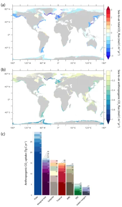
Figure 4. Global mean distribution of the simulated sea-to-air flux of (a) total carbon and (b) anthropogenic carbon over 1993–2012 as
mol C m−2yr−1in the global coastal ocean segmented following MARCATS from LA13. (c) Bar chart of the anthropogenic carbon uptake in
Tg C yr−1according to the MARCATS classification. Abbreviations are included for eastern boundary current (EBC) and western boundary
current (WBC). Links between numbers and regions are reported in Table 2. Interactive illustrations can be found at http://lsce-datavisgroup. github.io/CoastalCO2Flux/.
the Arctic polar regions, the simulated uptake is too low, with 52 Tg C yr−1from the model vs. 86 Tg C yr−1from LA14.
3.2.2 Anthropogenic CO2
The anthropogenic FCO2 is computed as the difference
be-tween the total flux (historical simulation) and natural flux (control simulation). When integrated over the global coastal ocean, the mean anthropogenic flux from 1993 to 2012 is 0.10 ± 0.01 Pg C yr−1. That amounts to 4.5 % of the simu-lated global anthropogenic carbon uptake, substantially less than the 7.5 % proportion of the coastal-to-global ocean
sur-face areas. During the period 1950–2000, the uptake of an-thropogenic carbon by the coastal ocean essentially grows linearly as it does for the global ocean. That is, it grows at a nearly constant rate of 0.0015 Pg C yr−2, which is 4.4 % of the rate for the global ocean increase in anthropogenic car-bon uptake over the same period (Fig. 2).
All MARCATS regions absorb anthropogenic carbon at rates ranging from 0.01 mol C m−2yr−1 for the Baltic Sea to 0.86 mol C m−2yr−1for the South Greenland region (Ta-ble 2 and Fig. 4.b). By class, the strongest specific fluxes of anthropogenic carbon into the ocean occur in the boundary
(a) (b) Total Anthropogenic Natural Total Anthropogenic Natural
Figure 5. Zonal-mean, sea-to-air fluxes of total, anthropogenic, and
natural CO2(mol C m−2yr−1) given as the average over 1993–2012
for (a) the coastal ocean and (b) the global ocean. Shaded areas indicate the standard deviation of environmental variability of all ocean grid cells within each latitudinal band. Interannual variations are not shown.
current regions, namely the EBC and WBC, with 0.42 and 0.48 mol C m−2yr−1 respectively. Conversely, the weakest anthropogenic carbon uptake occurs in the tropical margins and the Indian margins with 0.22 and 0.24 mol C m−2yr−1 respectively. But specific fluxes can be misleading. Although the polar and subpolar margins do not have the highest spe-cific fluxes, their integrated uptake of anthropogenic carbon is large because of their large surface areas (Fig. 4b and c). Together they absorb 46 Tg C yr−1, which is 45 % of total up-take of anthropogenic carbon by the global coastal ocean.
These results emphasize that there is no link between an-thropogenic and total carbon fluxes when comparing patterns between regions. For example, even though the EBC and WBC regions are the most efficient regions in anthropogenic carbon uptake (both above 0.4 mol C m−2yr−1), their be-haviour differs greatly in terms of the flux of total carbon, i.e. −1.65 vs. −0.12 mol C m−2yr−1 respectively (Fig. 7). The same lack of correlation between anthropogenic and
to-−4 −3 −2 −1 0 1 2 3 −4 −3 −2 −1 0 1 2 3
Observed CO2 flux (mol C m−2 y−1)
Simulated CO 2 flux (mol C m −2 y −1) EBC WBC Polar Subpolar Tropical Indian Marginal
Figure 6. Simulated vs. observed MARCATS sea-to-air flux of total
carbon in (a) mol C m−2yr−1and (b) Tg C yr−1. Vertical error bars
show the standard deviation from the 1993–2012 interannual vari-ability for model results and the horizontal bars correspond to the 1990–2011 variability from computational methods used in LA14 for observation-based estimates. Here, regression line (grey dotted) have y intercepts forced to 0. All MARCATS regions have been used except the Black Sea, the Persian Gulf (no data estimate), and the Sea of Okhotsk (see text).
-25 -20 -15 -10 -5 0 5
EBC WBC Indian Marginal Tropical Subpolar Polar
MARCATS classes Sea −to −air CO 2 flux (Tg C y −1 )
Figure 7. Box plots of the simulated sea-to-air CO2 fluxes
(Tg C yr−1) grouped into the MARCATS classes of the coastal
ocean. Black boxes indicate total fluxes, and red boxes indicate an-thropogenic fluxes. Shown are the lowest estimate, the first quar-tile, the median, the third quarquar-tile, and the highest estimate for each class.
tal flux patterns is even clearer in the zonal mean distributions (Fig. 5). For instance, the specific fluxes of anthropogenic carbon into the coastal ocean between 55◦S and 90◦N are nearly uniform, remaining near −0.5 mol C m−2yr−1; con-versely, the total carbon fluxes vary greatly between −2
2
and +0.5 mol C m−2yr−1. These variations in the total car-bon flux are dictated by variations in the natural carcar-bon flux (Fig. 5).
4 Discussion
4.1 Comparison with previous coastal estimates
4.1.1 Total flux
Our mean simulated uptake of total carbon by the global coastal ocean over 1993 to 2012 is 0.27 ± 0.07 Pg C yr−1, which falls within the range of previous data-based esti-mates of 0.2–0.4 Pg C yr−1 (Borges et al., 2005; Cai et al., 2006; Chen and Borges, 2009; Laruelle et al., 2010; Cai, 2011; Chen et al., 2013; Laruelle et al., 2014). Out of those, estimates provided since 2011 gather closer to the lower limit, e.g. the estimate of 0.2 Pg C yr−1 from LA14, as is also the case for our model-based estimate. Some aspects of the LA14 data-based approach are shared by our model-based approach, i.e. the same reference period, essentially the same definition of the coastal ocean, and the same cor-rection for the effect of sea ice cover on FCO2. LA14 is the
first observation-based study to take into account this sea ice effect for coastal-ocean FCO2 estimates at the global scale.
Using a box model, Andersson and Mackenzie (2004) and Mackenzie et al. (2004) estimated that the global coastal ocean acted as a carbon source to the atmosphere prior to industrialization; however, they also estimate that industrial-ization has recently led to a reversal in the sign of this flux (the global coastal ocean became a carbon sink) mainly due to the enhancement of NEP from increased riverine inputs. In contrast, our model simulations indicate that the preindus-trial coastal ocean was already a carbon sink, and that this sink has strengthened over the industrial period. This dis-crepancy appears to be explained by different definitions of the coastal ocean. Both the box model and our 3-D model include the distal coastal zone, but only the box model in-cludes the proximal coastal zone (bays, estuaries, deltas, la-goons, salt marshes, mangroves, and banks). That proximal zone is known generally as a strong source of carbon to the atmosphere (Rabouille et al., 2001).
The model representation of riverine DOC input and its instantaneous remineralization has potential implications for our estimates of total FCO2. In the Amazon plume for
in-stance, we underestimate CO2absorption because of this
in-stantaneous addition of DIC without input of alkalinity. How-ever this assumption has no direct implication on our anthro-pogenic FCO2estimates.
Furthermore, our simplified representation of sedimentary processes affects simulated total CO2fluxes (Krumins et al.,
2013; Soetaert et al., 2000). First, the model lacks an ex-plicit representation of sedimentary processes. Thus it can-not reproduce the temporal dynamics of interactions between
sediments and the overlying water column, e.g. resulting in potential delays between sediment burial and remineraliza-tion. Second, our model neglects any alkalinity source from sediment anaerobic degradation, such as denitrification and sulfate reduction of deposited organic matter. Even if not well constrained (Chen, 2002; Thomas et al., 2009; Hu and Cai, 2011; Krumins et al., 2013), this source of alkalinity could partially balance the total CO2 uptake of the coastal
ocean. However, the simplified representation of these sed-iment processes has no direct effect on our anthropogenic FCO2 estimates.
4.1.2 Anthropogenic flux
The strongest specific fluxes of anthropogenic carbon into the ocean occur in the boundary current regions, namely the EBC and WBC. Indeed, these regions show significant verti-cal and lateral mixing features such as filaments and eddies from the strong adjacent western boundary currents and up-welling from Eastern boundary upup-welling systems (EBUS). Those physical processes lead to the deepening of the mixed layer depth, export of the absorbed anthropogenic carbon from shallow water to deeper water layers, and its transfer to the adjacent open ocean.
Our estimate of the simulated anthropogenic carbon up-take of 0.10 Pg C yr−1for the global coastal ocean (Fig. 9) is about half that found by Wanninkhof et al. (2013) for a sim-ilar period. The latter study estimates coastal anthropogenic CO2uptake by extrapolating specific FCO2from the adjacent
open ocean into coastal areas, exploiting coarse-resolution models and data. To compare approaches, we applied the Wanninkhof et al. (2013) extrapolation method to our model output; we found the same result as theirs for global coastal-ocean uptake of anthropogenic CO2 (0.18 Pg C yr−1). Thus
the extrapolation technique leads to an overestimate of an-thropogenic CO2uptake in the model’s global coastal ocean.
Nonetheless, the Wanninkhof et al. (2013) estimate for the anthropogenic carbon uptake by the coastal ocean was used by Regnier et al. (2013) for their coastal carbon budget. That budget also accounts for the increase in river discharge of carbon (0.1 Pg C yr−1) and nutrients during the industrial era, which promotes organic carbon production, some of which is buried in the coastal zone (up to 0.15 Pg C yr−1). Unfor-tunately, these numbers remain particularly uncertain. Hence we have chosen to ignore them, adopting the conventional definition of anthropogenic carbon in the ocean used by pre-vious global-ocean model studies, namely that anthropogenic carbon comes only from the direct geochemical effect of the anthropogenic increase in atmospheric CO2 and its
subse-quent invasion into the ocean. The future challenge of im-proving estimates of changes and variability in riverine de-livery of carbon and nutrient and sediment burial is critical to refine land contributions to the coastal-ocean carbon bud-get.
Our estimate of 0.10 Pg C yr−1for the anthropogenic FCO2
into the coastal ocean is 40 % less than the 0.17 Pg C yr−1 es-timated by Borges (2005) from Andersson and Mackenzie (2004) and Mackenzie et al. (2004). Causes for this differ-ence may stem from (1) the different definitions of the coastal ocean (proximal coastal zone included in the box model but not the 3-D model), (2) the different approaches (uniform coastal ocean in the box model but not in the 3-D model), and (3) the role of sediments (pore waters included in the box model but neglected in the 3-D model).
4.2 Coastal vs. open ocean
Patterns in our simulated total FCO2 in the coastal ocean
generally follow those for the open ocean, with net carbon sources in the low latitudes and carbon sinks in the middle to high latitudes (Fig. 5). The same tendency was pointed out by Gruber (2014) when discussing the LA14 data-based fluxes. The patterns in our simulated total CO2 flux are mainly
driven by patterns in the natural CO2flux both in the coastal
and open oceans (Fig. 5). Yet the pattern for anthropogenic CO2flux differs greatly from that of natural CO2, having its
strongest uptake in the Southern Ocean in both the open and coastal oceans, i.e. where zonally averaged specific uptake reaches up to 1.5 mol C m−2yr−1. The bathymetry of MAR-CATS regions around the Antarctic continent is much deeper than in the other coastal regions (500 m vs. 160 m for the global coastal ocean); this probably reduces the contrast be-tween the coastal and open ocean in the Southern Ocean and explains the similarities of anthropogenic carbon uptake rates there.
Despite large-scale similarities between coastal- and open-ocean fluxes of total carbon, some coastal regions differ substantially from those in the adjacent open-ocean waters (Fig. 3a). These local differences are particularly apparent around coastal upwelling systems, i.e. in the western Ara-bian Sea and in eastern boundary upwelling systems (EBUS), such as the Peruvian upwelling current, the Moroccan up-welling, and the south-western Africa upwelling. Some of these coastal regions act as strong total carbon sources, with mean carbon fluxes of up to 1.44 mol C m−2yr−1, whereas surrounding open-ocean waters exhibit little FCO2 (fluxes
close to 0 mol C m−2yr−1). Other regions also exhibit large contrast between their coastal waters and the adjacent open ocean, including the tropical western Atlantic where there is a massive loss of carbon at the location of the Amazon river discharge. However the carbon sink in the Amazon river plume reported in Lefèvre et al. (2010) is not repro-duced in our model. This discrepancy may be due to the mod-elled instantaneous remineralization of land-derived DOC or to shortcomings in the model representation of sedimentary processes.
A key finding of our model study is that the flux of an-thropogenic CO2 into the coastal ocean (0.10 Pg C yr−1) is
half the previous estimate (Wanninkhof et al., 2013).
Un-like in that study, our specific flux of anthropogenic CO2is
substantially lower for the global coastal ocean than for the global open ocean (i.e. −0.31 vs. −0.54 mol C m−2yr−1for the 1993–2012 average). Although the coastal-ocean surface area is 7.5 % of the global ocean, it absorbs only 4.5 % of the globally integrated flux of anthropogenic carbon into the ocean.
Our estimate for coastal-ocean uptake of anthropogenic carbon is 10 times smaller than the 1 Pg C yr−1estimate by Tsunogai et al. (1999) associated with their proposed conti-nental shelf pump (CSP). However, Tsunogai’s CSP is based on contemporary measurements and thus concerns total car-bon, not the anthropogenic change. That nuance is critical be-cause contemporary estimates of fluxes are not directly com-parable to anthropogenic fluxes nor global budgets of car-bon from the IPCC and the Global Carcar-bon Project, both fo-cused on the anthropogenic change. Unfortunately Tsunogai et al. (1999) prompted confusion by stating that their total carbon flux into the coastal ocean was equivalent to half of the global-ocean uptake of anthropogenic carbon. The same confusion prompted Thomas et al. (2004) to emphasize that the coastal ocean contributes more to the global carbon bud-get than expected from its surface area.
The lower specific flux of anthropogenic CO2 into the
global coastal ocean relative to the average for the open ocean could have two causes: (1) physical factors (e.g. if vertical mixing in the coastal ocean is relatively weak or if there is a bottleneck in the offshore transport carbon) and (2) chemical factors, if coastal waters have a lower chemi-cal capacity to absorb anthropogenic carbon (lower carbon-ate ion concentration, higher Revelle factor Rf).
To assess how Rfdiffers between coastal- and open-ocean
surface waters, we computed it using CO2SYS from sim-ulated sea surface temperature, salinity, alkalinity, and DIC for the model years 1993–2012. Thus we computed mean Revelle factors of 12.5 for the global coastal ocean, 10.9 for the global ocean, 9.2 for the tropical oceans (30◦S–30◦N), and 12.8 for the Southern Ocean (90–30◦S). These tenden-cies are persistent. During the period 1910–2012, the aver-age coastal-ocean Revelle factor remains 15 % larger than for the open ocean. Hence average surface waters in the model’s coastal ocean have a lower chemical capacity to take up an-thropogenic carbon relative to average surface waters of the global ocean. That finding is consistent with the lower simu-lated specific fluxes of anthropogenic carbon into the coastal ocean. Yet it is not only the chemical capacity that matters. For example, despite similar chemical capacities, the specific flux of anthropogenic carbon into Southern Ocean is more than twice that of the global coastal ocean. Thus, we must turn to physical factors to help explain the lower efficiency of the coastal ocean to take up anthropogenic carbon.
Out of the 0.10 Pg C yr−1 absorbed by the coastal ocean, we find that only 70 % (i.e. 0.07 Pg C yr−1) is transferred to the open ocean (Fig. 9). Thus 0.03 Pg C yr−1 of anthro-pogenic carbon accumulates in the coastal-ocean water
col-2 Long itude Latitude Residenc e time (mon th)
Figure 8. Global distribution of simulated residence time (month) for the global coastal ocean segmented following Laruelle et al. (2013).
0.07 0.10 0.03 0.05 COASTAL OCEAN ATMOSPHERE OPEN OCEAN 2.16 2.23 2.4 2.26 2.5 0.2
Simulated and data-‐based anthropogenic carbon
flux and accumula>on rate on 1993-‐2012 (Pg C yr-‐1)
0 Rivers 0.1 2.3 0 0.15 0 0 Sediments 0.1
Figure 9. Transfer of anthropogenic carbon between the atmo-sphere, coastal ocean, and open ocean along with increases in the corresponding inventory in each reservoir, given as the average of
simulated values over 1993–2012. All results are in Pg C yr−1.
Sim-ulated results are shown as dark numbers in boxes and adjacent numbers (grey italic) indicate data-based estimates for the 2000– 2010 average (Regnier et al., 2013).
umn during the 1993–2012 period. That simulated accu-mulation is not significantly different from the estimate of 0.05 ± 0.05 Pg C yr−1 from Regnier et al. (2013). The ac-cumulation in the coastal ocean is effective over the entire period (1910–2012) as the uptake of anthropogenic carbon by the global coastal ocean is always inferior to its cross-shelf export (Fig. 10). To gain insight into this cross-cross-shelf exchange, we computed the simulated mean water residence times for each MARCATS region (Fig. 8). Residence times for most coastal regions are of the order of a few months or less, except for Hudson Bay, the Baltic Sea, and the Persian Gulf. The latter three regions are generally more confined
and we expect longer residence times, although our model simulations were never designed to simulate these regions ac-curately. Generally, our simulated residence times are shorter than what has been published for similarly defined coastal re-gions, although methods differ substantially (Jickells, 1998; Men and Liu, 2014; Delhez et al., 2004). Despite these short residence times, the cross-shelf export of anthropogenic car-bon is unable to keep up with the increasing air–sea flux of anthropogenic carbon (Fig. 10). This may be explained by the open-ocean waters that are imported to the coastal ocean being already charged with anthropogenic carbon, thus limit-ing further uptake in the coastal zone. This accumulation rate of anthropogenic carbon in the coastal ocean contrasts with the lower simulated proportion that remains in the mixed layer of the global ocean. Using a coarse-resolution global model, Bopp et al. (2015) showed that on average for the global ocean, only ∼10 % of the anthropogenic carbon that crosses the air–sea interface accumulates in the seasonally-varying mixed layer. The CSP hypothesis from Tsunogai et al. (1999) assumes that much of the 1 Pg C yr−1 of total carbon absorbed by the coastal ocean is exported to the deep ocean. Also assuming that the CSP operates equally in all shelf regions across the world, Yool and Fasham (2001) used a coarse- resolution global model to estimate that 53 % of the coastal uptake is exported to the open ocean. Yet they considered only natural carbon. Conversely, we focus purely on anthropogenic carbon. Our simulations suggest that 70 % of the anthropogenic carbon absorbed by the coastal ocean over 1993 to 2012 is transported offshore to the deeper open ocean.
1920 1940 1960 1980 2000 0 0.5 1 1.5 2 Time (year)
Anthropogenic carbon inventory (Pg C)
1920 1940 1960 1980 2000 0 0.02 0.04 0.06 0.08 0.1 0.12 Time (year)
Anthropogenic carbon flux (Pg C yr
−1) Cross−shelf DICant export
Coastal Cant uptake
Figure 10. Simulated temporal evolution of (a) coastal-ocean inventory of anthropogenic carbon given in Pg C and (b) anthropogenic CO2
(Cant) uptake by the global coastal ocean and global cross-shelf export of anthropogenic carbon (DICant) given in Pg C yr−1.
5 Conclusions
The goal of this study was to estimate the anthropogenic CO2
flux from the atmosphere to the coastal ocean, both glob-ally and regionglob-ally, using an eddying global-ocean model, making 143-year simulations forced by atmospheric reanal-ysis data and atmospheric CO2. We first evaluated the
sim-ulated air–sea fluxes of total CO2for 45 coastal regions and
found a correlation coefficient R of 0.8 when compared to observation-based estimates. Then we estimated the average simulated anthropogenic carbon uptake by the global coastal ocean over 1993–2012 to be 0.10 ± 0.01 Pg C yr−1, equiva-lent to 4.5 % of global-ocean uptake of anthropogenic CO2,
an amount less than expected based on the surface area of the global coastal ocean (7.5 % of the global ocean). Fur-thermore, our estimate is only about half of that estimated by Wanninkhof et al. (2013), whose budget was based on extrapolating adjacent open-ocean data-based estimates of the specific flux into the coastal ocean. We attribute our lower specific flux of anthropogenic carbon into the global coastal ocean mainly to the model’s associated offshore car-bon transport, which is not strong enough to reduce surface levels of anthropogenic DIC (and thus anthropogenic pCO2)
to levels that are as low as those in the open ocean (on aver-age). Whether or not our model provides a realistic estimate of offshore transport at the global scale is a critical question that demands further investigation.
Clearly, our approach is limited by the extent to which the coastal ocean is resolved. Our model’s horizontal resolu-tion does not allow it to fully resolve some fine-scale coastal processes such as tides, which affect FCO2 at tidal fronts
(Bianchi et al., 2005). Model resolution is also inadequate to fully resolve mesoscale and submesoscale eddies and asso-ciated upwelling. Moreover, in the midlatitudes with a water depth of 80 m, the first baroclinic Rossby radius (the domi-nant scale affecting coastal processes) is around 200 km, but
the latter falls below 10 km on Arctic shelves (Holt et al., 2014; Nurser and Bacon, 2014). Thus the higher latitudes need much finer resolution (Holt et al., 2009).
Yet all model studies must weigh the costs and bene-fits of pushing the limits toward improved realism. Our ap-proach has been to use a model that takes only a first step into the eddying regime in order to be able to achieve long physical-biogeochemical simulations with atmospheric CO2
increasing from preindustrial levels to today. It represents a step forward relative to previous studies with typical coarse-resolution ocean models (around 2◦ horizontal resolution), which may be considered to be designed exclusively for the open ocean. In the coming years, increasing computational resources will allow further increases in spatial resolution and a better representation of the coastal ocean in global ocean carbon cycle models.
Improvements will also be needed in terms of the mod-elled biogeochemistry of the coastal zone. Most global-scale biogeochemical models neglect river input of nutrients and carbon. Although that is taken into account in our simula-tions, the river input forcing is constant in time (Aumont et al., 2015). Seasonal and higher frequency variability in car-bon and nutrient river input (e.g. from floods and droughts) is substantial as are typical anthropogenic trends. For sim-plicity, virtually all global-scale models neglect sediment re-suspension and early diagenesis in the coastal zone. Those processes in some coastal areas may well alter nutrient avail-ability, surface DIC, and total alkalinity, which would affect FCO2. In addition, in the coastal zone, one must eventually
go beyond the classic definition of anthropogenic carbon, i.e. the change due only to the direct influence of the anthro-pogenic increase in atmospheric CO2on the FCO2 and ocean
carbonate chemistry. Changes in other human-induced per-turbations may be substantial. For example, future research should better assess potential changes in sediment burial of carbon in the coastal zone during the industrial era, estimated
2
at up to 0.15 Pg C yr−1 but with large uncertainty (Regnier et al., 2013).
To improve understanding of the critical land–ocean con-nection and its role in carbon and nutrient exchange, we call for a long-term effort to exploit the latest, global-scale, high-resolution, ocean general circulation models, adding ocean biogeochemistry, and improving them to better represent the coastal and open oceans together as one seamless system.
6 Code availability
The code of the NEMO ocean model version 3.2 is available under CeCILL license at http://www.nemo-ocean.eu.
7 Data availability
As a supplementary material, we provide the simulated air-sea total and natural CO2fluxes over the 1993–2012 period
Cflux.nc), model grid parameters (bg-2016-57-grid.nc), and times series for area-integrated CO2fluxes
(bg-2016-57-timeseries.txt).
Acknowledgements. We are grateful to the associate editor
J. Middelburg for managing the peer-reviewing process and to two referees, N. Gruber and P. Regnier, for their helpful comments. We thank G. G. Laruelle for providing the raw data version of the Laruelle et al. (2014) database, and we are grateful to C. Nangini and P. Brockmann for their help with the GIS analysis, data treatment, and data visualization. We also thank J. Simeon for the first implementation of the ORCA05-PISCES model. The research leading to these results was supported through the EU FP7 project CARBOCHANGE (grant 264879), the EU H2020 project CRESCENDO (grant 641816), and the EU H2020 project C-CASCADES (Marie Sklodowska-Curie grant 643052). Simulations were made using HPC resources from GENCI-IDRIS (grant x2015010040). Timothée Bourgeois was funded through a scholarship cosupported by DGA-MRIS and CEA scholarship. Edited by: J. Middelburg
Reviewed by: N. Gruber and P. Regnier
References
Allen, J. I., Blackford, J., Holt, J., Proctor, R., Ashworth, M., and Siddorn, J.: A highly spatially resolved ecosystem model for the North West European Continental Shelf, Sarsia, 86, 423–440, 2001.
Andersson, A. J. and Mackenzie, F. T.: Shallow-water oceans: a
source or sink of atmospheric CO2?, Front. Ecol. Environ., 2,
348–353, 2004.
Artioli, Y., Blackford, J. C., Nondal, G., Bellerby, R. G. J., Wake-lin, S. L., Holt, J. T., Butenschön, M., and Allen, J. I.:
Het-erogeneity of impacts of high CO2 on the North Western
Eu-ropean Shelf, Biogeosciences, 11, 601–612, doi:10.5194/bg-11-601-2014, 2014.
Astor, Y. M., Lorenzoni, L., Thunell, R., Varela, R., Muller-Karger, F., Troccoli, L., Taylor, G. T., Scranton, M. I., Tappa, E., and Rueda, D.: Interannual variability in sea surface temperature and
FCO2 changes in the Cariaco Basin, Deep-Sea Res. Pt. II, 93,
33–43, 2013.
Atlas, R., Hoffman, R. N., Ardizzone, J., Leidner, S. M., Jusem, J. C., Smith, D. K., and Gombos, D.: A Cross-calibrated, Multi-platform Ocean Surface Wind Velocity Product for Meteorolog-ical and Oceanographic Applications, Bull. Am. Meteorol. Soc., 92, 157–174, 2011.
Aumont, O. and Bopp, L.: Globalizing results from ocean in situ iron fertilization studies, Global Biogeochem. Cy., 20, GB2017, doi:10.1029/2005GB002591, 2006.
Aumont, O., Ethé, C., Tagliabue, A., Bopp, L., and Gehlen, M.: PISCES-v2: an ocean biogeochemical model for carbon and ecosystem studies, Geosci. Model Dev., 8, 2465–2513, doi:10.5194/gmd-8-2465-2015, 2015.
Bakker, D. C. E., Pfeil, B., Smith, K., Hankin, S., Olsen, A., Alin, S. R., Cosca, C., Harasawa, S., Kozyr, A., Nojiri, Y., O’Brien, K. M., Schuster, U., Telszewski, M., Tilbrook, B., Wada, C., Akl, J., Barbero, L., Bates, N. R., Boutin, J., Bozec, Y., Cai, W.-J., Castle, R. D., Chavez, F. P., Chen, L., Chierici, M., Cur-rie, K., de Baar, H. J. W., Evans, W., Feely, R. A., Fransson, A., Gao, Z., Hales, B., Hardman-Mountford, N. J., Hoppema, M., Huang, W.-J., Hunt, C. W., Huss, B., Ichikawa, T., Johan-nessen, T., Jones, E. M., Jones, S. D., Jutterström, S., Kitidis, V., Körtzinger, A., Landschützer, P., Lauvset, S. K., Lefèvre, N., Manke, A. B., Mathis, J. T., Merlivat, L., Metzl, N., Murata, A., Newberger, T., Omar, A. M., Ono, T., Park, G.-H., Pater-son, K., Pierrot, D., Ríos, A. F., Sabine, C. L., Saito, S., Salis-bury, J., Sarma, V. V. S. S., Schlitzer, R., Sieger, R., Skjelvan, I., Steinhoff, T., Sullivan, K. F., Sun, H., Sutton, A. J., Suzuki, T., Sweeney, C., Takahashi, T., Tjiputra, J., Tsurushima, N., van Heuven, S. M. A. C., Vandemark, D., Vlahos, P., Wallace, D. W. R., Wanninkhof, R., and Watson, A. J.: An update to the Sur-face Ocean CO2 Atlas (SOCAT version 2), Earth Syst. Sci. Data, 6, 69–90, doi:10.5194/essd-6-69-2014, 2014.
Barnier, B., Madec, G., Penduff, T., Molines, J. M., Treguier, A. M., Le Sommer, J., Beckmann, A., Biastoch, A., Böning, C., Dengg, J., Derval, C., Durand, E., Gulev, S., Remy, E., Talandier, C., Theetten, S., Maltrud, M., McClean, J., and De Cuevas, B.: Impact of partial steps and momentum advection schemes in a global ocean circulation model at eddy-permitting resolution, Ocean Dynam., 56, 543–567, 2006.
Bauer, J. E., Cai, W.-J., Raymond, P. A., Bianchi, T. S., Hopkinson, C. S., and Regnier, P.: The changing carbon cycle of the coastal ocean, Nature, 504, 61–70, 2013.
Bianchi, A. A., Bianucci, L., Piola, A. R., Pino, D. R., Schloss, I., Poisson, A., and Balestrini, C. F.: Vertical stratification and
air-sea CO2fluxes in the Patagonian shelf, J. Geophys. Res.-Ocean.,
110, 1–10, 2005.
Bopp, L., Lévy, M., Resplandy, L., and Sallée, J. B.: Pathways of anthropogenic carbon subduction in the global ocean, Geophys. Res. Lett., 42, 6416–6423, 2015.
Borges, A. V.: Do we have enough pieces of the jigsaw to integrate
CO2fluxes in the coastal ocean?, Estuaries, 28, 3–27, 2005.
Borges, A. V., Delille, B., and Frankignoulle, M.: