HAL Id: cea-01135424
https://hal-cea.archives-ouvertes.fr/cea-01135424
Submitted on 25 Mar 2015
HAL is a multi-disciplinary open access
archive for the deposit and dissemination of
sci-entific research documents, whether they are
pub-lished or not. The documents may come from
teaching and research institutions in France or
abroad, or from public or private research centers.
L’archive ouverte pluridisciplinaire HAL, est
destinée au dépôt et à la diffusion de documents
scientifiques de niveau recherche, publiés ou non,
émanant des établissements d’enseignement et de
recherche français ou étrangers, des laboratoires
publics ou privés.
Revealing the cold dust in low-metallicity environments
A. Rémy-Ruyer, S. C. Madden, F. Galliano, S. Hony, M. Sauvage, G. J.
Bendo, Hervé Roussel, M. Pohlen, M. W. L. Smith, M. Galametz, et al.
To cite this version:
A. Rémy-Ruyer, S. C. Madden, F. Galliano, S. Hony, M. Sauvage, et al.. Revealing the cold dust in
low-metallicity environments. Astronomy and Astrophysics - A&A, EDP Sciences, 2013, 557, pp.A95.
�10.1051/0004-6361/201321602�. �cea-01135424�
DOI:10.1051/0004-6361/201321602 c
ESO 2013
Astrophysics
&
Revealing the cold dust in low-metallicity environments
I. Photometry analysis of the Dwarf Galaxy Survey with Herschel
?A. Rémy-Ruyer
1, S. C. Madden
1, F. Galliano
1, S. Hony
1, M. Sauvage
1, G. J. Bendo
2, H. Roussel
3, M. Pohlen
4,
M. W. L. Smith
4, M. Galametz
5, D. Cormier
1, V. Lebouteiller
1, R. Wu
1, M. Baes
6, M. J. Barlow
7, M. Boquien
8,
A. Boselli
8, L. Ciesla
9, I. De Looze
6, O. Ł. Karczewski
7, P. Panuzzo
10, L. Spinoglio
11, M. Vaccari
12,
C. D. Wilson
13, and the Herschel-SAG2 consortium
1 Laboratoire AIM, CEA, Université Paris Sud XI, IRFU/Service d’Astrophysique, Bât. 709, 91191 Gif-sur-Yvette, France
e-mail: [email protected]
2 UK ALMA Regional Centre Node, Jodrell Bank Centre for Astrophysics, School of Physics & Astronomy,
University of Manchester, Oxford Road, Manchester M13 9PL, UK
3 Institut d’Astrophysique de Paris, UMR 7095 CNRS, Université Pierre & Marie Curie, 98bis boulevard Arago, 75014 Paris, France 4 School of Physics & Astronomy, Cardiff University, The Parade, Cardiff, CF24 3AA, UK
5 Institute of Astronomy, University of Cambridge, Madingley Road, Cambridge CB3 0HA, UK 6 Sterrenkundig Observatorium, Universiteit Gent, Krijgslaan 281 S9, 9000 Gent, Belgium
7 Department of Physics and Astronomy, University College London, Gower St, London WC1E 6BT, UK
8 Laboratoire d’Astrophysique de Marseille − LAM, Université d’Aix-Marseille & CNRS, UMR 7326, 38 rue F. Joliot-Curie,
13388 Marseille Cedex 13, France
9 Department of Physics, University of Crete, 71003 Heraklion, Greece
10 GEPI, Observatoire de Paris, CNRS, Univ. Paris Diderot, Place Jules Janssen, 92190 Meudon, France 11 Instituto di Astrofisica e Planetologia Spaziali, INAF-IAPS, Via Fosso del Cavaliere 100, 00133 Roma, Italy 12 Physics Department, University of the Western Cape, Private Bag X17, 7535 Bellville, Cape Town, South Africa 13 Department of Physics & Astronomy, McMaster University, Hamilton Ontario L8S 4M1, Canada
Received 29 March 2013/ Accepted 18 June 2013
ABSTRACT
Context.We present new photometric data from our Herschel guaranteed time key programme, the Dwarf Galaxy Survey (DGS), dedicated to the observation of the gas and dust in low-metallicity environments. A total of 48 dwarf galaxies were observed with the PACS and SPIRE instruments onboard the Herschel Space Observatory at 70, 100, 160, 250, 350, and 500 µm.
Aims. The goal of this paper is to provide reliable far-infrared (FIR) photometry for the DGS sample and to analyse the FIR/submillimetre (submm) behaviour of the DGS galaxies. We focus on a systematic comparison of the derived FIR properties (FIR luminosity, LFIR, dust mass, Mdust, dust temperature, T, emissivity index, β) with more metal-rich galaxies and investigate the
detection of a potential submm excess.
Methods.The data reduction method is adapted for each galaxy in order to derive the most reliable photometry from the final maps. The derived PACS flux densities are compared with the Spitzer MIPS 70 and 160 µm bands. We use colour−colour diagrams to analyse the FIR/submm behaviour of the DGS galaxies and modified blackbody fitting procedures to determine their dust properties. To study the variation in these dust properties with metallicity, we also include galaxies from the Herschel KINGFISH sample, which contains more metal-rich environments, totalling 109 galaxies.
Results.The location of the DGS galaxies on Herschel colour−colour diagrams highlights the differences in dust grain properties
and/or global environments of low-metallicity dwarf galaxies. The dust in DGS galaxies is generally warmer than in KINGFISH galaxies (TDGS ∼ 32 K and TKINGFISH ∼ 23 K). The emissivity index, β, is ∼1.7 in the DGS, however metallicity does not make a
strong effect on β. The proportion of dust mass relative to stellar mass is lower in low-metallicity galaxies: Mdust/Mstar∼ 0.02% for
the DGS versus 0.1% for KINGFISH. However, per unit dust mass, dwarf galaxies emit about six times more in the FIR/submm than higher metallicity galaxies. Out of the 22 DGS galaxies detected at 500 µm, about 41% present an excess in the submm beyond the explanation of our dust SED model, and this excess can go up to 150% above the prediction from the model. The excess mainly appears in lower metallicity galaxies (12+ log(O/H) . 8.3), and the strongest excesses are detected in the most metal-poor galaxies. However, we also stress the need for observations longwards of the Herschel wavelengths to detect any submm excess appearing beyond 500 µm.
Key words.galaxies: ISM – galaxies: dwarf – galaxies: photometry – infrared: galaxies – infrared: ISM – dust, extinction
1. Introduction
The continuous interplay between stars and the interstellar medium (ISM) is one of the major drivers of galaxy evolution.
?
Tables 1−4 and Appendices are available in electronic form at http://www.aanda.org
The ISM is primarily composed of gas and dust, and it plays a key role in this evolution, as the repository of stellar ejecta and the site of stellar birth. It thus contains the imprint of the astrophysical processes occurring in a galaxy. Interstellar dust is present in most phases of the ISM, from warm ionized re-gions around young stars to the cores of dense molecular clouds.
Because dust is mainly formed from the available metals in the ISM, the dust content traces its internal evolution through metal enrichment. Dust thus influences the subsequent star formation and has a significant impact on the total spectral energy distri-bution (SED) of a galaxy: the absorbed stellar light by dust in the ultraviolet (UV) and visible wavelengths is re-emitted in the infrared (IR) domain by the dust grains. In our Galaxy, dust re-processes about 30% of the stellar power, and it can grow to as large as ∼99% in a starburst galaxy. Studying the IR emission of galaxies thus provides valuable information on the dust proper-ties of the galaxies and on their overall star formation activity.
Our Galaxy, as well as other well studied local Universe galaxies, provide various observational benchmarks to calibrate the physical dust properties around solar metallicity. However, for galaxies of the high-redshift Universe, dust properties are still poorly known, due to observational constraints and to the unsure variations in dust properties as the metallicity decreases. Because of their low metal abundance and active star formation, dwarf galaxies of the local Universe are ideal laboratories for studying star formation and its feedback on the ISM in con-ditions that may be representative of different stages in early Universe environments.
From IRAS to Spitzer, many studies have been dedicated to dwarf galaxies over the past decades, and have uncovered pe-culiar ISM properties compared to their metal-rich counterparts. Among these, are the following:
Overall warmer dust: the SEDs in some low-metallicity star-forming dwarf galaxies often peak at shorter wavelengths, some-times well below 100 µm, whereas for more metal-rich galaxies, the peak of the SED is around 100−200 µm (Galliano et al. 2003,
2005;Walter et al. 2007;Engelbracht et al. 2008;Galametz et al. 2009). This is a consequence of the harder interstellar radiation field (ISRF) interacting with the porous ISM of dwarf galaxies (e.g.Madden et al. 2006).
Weak mid infrared (MIR) aromatic features: the polycyclic aromatic hydrocarbons (PAHs) are often barely detected, if at all, in these galaxies (e.g. Sauvage et al. 1990;Madden 2000;
Boselli et al. 2004;Engelbracht et al. 2005). The combination of young star clusters and metal-poor ISM creates a harder galaxy-wide radiation field compared to that of our Galaxy. The paucity of dust allows the harder UV photons to travel deeper into the ISM and destroy PAH molecules by photoevaporation or pho-todissociation (Galliano et al. 2003,2005;Madden et al. 2006). The dearth of PAH features in dwarf galaxies has also been ex-plained by the destruction of the molecules by supernovae (SN) shocks (O’Halloran et al. 2006) or by a delayed carbon injection in the ISM by asymptotic giant branch (AGB) stars (Galliano et al. 2008).
The submillimetre (submm) excess: an excess emission, un-accountable by usual SED models, is appearing in the
far-infrared (FIR) to submm/millimetre (mm) domain for some
dwarf galaxies (Galliano et al. 2003,2005;Galametz et al. 2009;
Bot et al. 2010;Grossi et al. 2010). An excess emission has also been observed in our Galaxy with COBE (Reach et al. 1995) but with an intensity less pronounced compared to that found in low-metallicity systems. Dumke et al.(2004);Bendo et al.(2006);
Zhu et al.(2009) found a submm excess in some low-metallicity spiral galaxies as well. The discovery of this excess renders even more uncertain the determination of a quantity as fundamental as the dust mass.
The faint CO emission: CO is difficult to observe in dwarf galaxies (i.e. Leroy et al. 2009; Schruba et al. 2012), and the determination of the molecular gas reservoir at low metallici-ties through the usual CO-to-H2 conversion factor is still very
uncertain. The dependence of the CO-to-H2conversion factor on
metallicity has been studied extensively (Wilson 1995; Boselli et al. 2002; Leroy et al. 2011; Schruba et al. 2012) but have been limited to metallicities greater than ∼1/5 Z 1 due to the
difficulty of detecting CO at lower metallicities. This renders accurate determinations of gas-to-dust mass ratios (G/D) very difficult, as H2may account for a significant fraction of the total
(atomic HI and molecular H2) gas mass. We now believe that the
structure of molecular clouds in dwarf galaxies is very different from that of metal-rich systems, and that CO does not trace the full molecular gas reservoir. A potentially large reservoir of CO-dark molecular gas could exist in low-metallicity galaxies, trace-able by the FIR cooling line [CII] (Poglitsch et al. 1995;Israel et al. 1996;Madden et al. 1997,2012), or by neutral carbon [CI] (Papadopoulos et al. 2004;Wilson 2005).
The wavelength ranges and sensitivities covered by Spitzer, Infrared Space Observatory (ISO) and IRAS do not sample the cold dust component of the dust SED beyond 160 µm. Some ground-based telescopes such as JCMT, APEX, SEST, IRAM could detect the cold dust beyond 160 µm, but because of sen-sitivity limitations, accurate measures of the photometry could only be obtained for the brightest and highest metallicity dwarf galaxies. The Herschel Space Observatory (Pilbratt et al. 2010), launched in 2009, is helping to fill this gap and complete our view of dust in galaxies by constraining the cold dust contri-bution. Herschel covers a wide range of wavelengths in the FIR and submm, with unprecedented resolution: its 3.5 m di-ameter mirror is the largest ever launched in space so far for this wavelength range. Herschel carries three instruments among which are the Photodetector Array Camera and Spectrometer (PACS −Poglitsch et al. 2010) and the Spectral and Photometric Imaging REceiver (SPIRE −Griffin et al. 2010), both imaging photometres and medium resolution spectrometres. The PACS and SPIRE photometres in combination cover a 70 to 500 µm range, and the spectrometres together cover 55 to 670 µm.
We focus here on local dwarf galaxies by presenting new re-sults of the Herschel guaranteed time key progam, the Dwarf
Galaxy Survey (DGS − P.I. Madden; Madden et al. 2013).
Dwarf galaxies are studied here in a systematic way, enabling us to derive general properties that are representative of these systems. We will focus our study on overall dust properties and look at the submm excess. We present the observed sample and the data reduction processes in Sect.2. We then present the flux extraction method and the flux catalogues for the whole sam-ple in Sect.3. Section4is dedicated to the comparison of the dwarf galaxies with more metal-rich environments, first qualita-tively with colour−colour diagrams, and then quantitaqualita-tively with modified blackbody fits. We also inspect a sub-sample of galax-ies presenting a submm excess. Throughout this last section we compare our results with those from another Herschel sample, KINGFISH (Kennicutt et al. 2011), which is probing predomi-nantely more metal-rich environments, in order to study the var-ious overall effects of metallicity on the derived dust properties.
2. Observations and data reduction
2.1. The Dwarf Galaxy Survey with Herschel 2.1.1. Sample
The DGS aims at studying the gas and dust properties in low-metallicity ISMs with the Herschel Space Observatory. It is a
1 Throughout, we assume (O/H)
= 4.90 × 10⁴, i.e., 12+ log(O/H) =
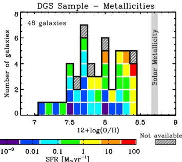
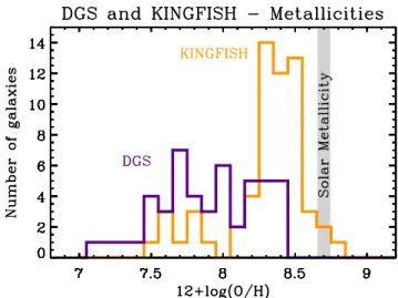
Fig. 1.Metallicity distribution of the DGS sample from 12+ log(O/H) = 7.14 to 8.43. Solar metallicity is indicated here as a guide to the eye. The pre-Herschel star formation rate (SFR) distribution is also indicated by the colour code. They have been converted from LTIR(Spitzer) with the
Kennicutt(1998) law, and are given inMadden et al.(2013). When no IR data was available, Hα or Hβ emission lines were used and con-verted to SFR (Kennicutt 1998). The dashed cells indicate that none of these data were available for the galaxy. The most actively star-forming galaxy (in red) corresponds to the starburst luminous infrared galaxy (LIRG) Haro 11.
photometric and spectroscopic survey of 50 dwarf galaxies at FIR and submm wavelengths (Madden et al. 2013). For a more detailed description of the general goals of the survey and the source selection process, see the Dwarf Galaxy Survey Overview by Madden et al.(2013). Here, we focus on the 48 targets for which complete photometry was obtained. The names, positions, distances and metallicities of the DGS galaxies are listed in Table1(fromMadden et al. 2013).
These targets span a wide range in metallicity from 12+ log(O/H) = 7.14 to 8.43, including I Zw 18 with Z ∼ 1/40 Z
(Lequeux et al. 1979; Izotov et al. 1999) which is one of the most metal-poor galaxies in the local Universe known to date (see Fig.1for the metallicity distribution of the DGS targets).
2.1.2. Observations
The Dwarf Galaxy Survey was granted ∼230 h of observations, part of which were used to observe the sample with the two Herschelimaging photometres: all of them (48) with PACS at 70, 100 and 160 µm and 41 with SPIRE at 250, 350 and 500 µm. Seven sources were not observed with SPIRE because they were predicted to be too faint for SPIRE. The full width at half maxi-mum (FWHM) of the beam in each band is 5.6, 6.8, 11.42, 18.2,
24.9, 36.3003at 70, 100, 160, 250, 350 and 500 µm respectively.
Most of the sources have also been observed by the PACS spec-trometre in order to complement the photometry (e.g. Cormier et al. 2011,2012;Lebouteiller et al. 2012;Madden et al. 2013; Cormier et al., in prep.).
2 The PACS Observers’ Manual is available at http://herschel.
esac.esa.int/Docs/PACS/pdf/pacs_om.pdf
3 The SPIRE Observers’ Manual is available athttp://herschel.
esac.esa.int/Docs/SPIRE/pdf/spire_om.pdf
For all of our galaxies, the PACS photometry observations have been done in the PACS scan-map mode at a medium scan speed (2000/s). The SPIRE observations have been made using the SPIRE large and small scan-map modes, depending on the source sizes, at the nominal scan speed (3000/s).
Substantial ancillary data are available over a large wave-length range, from UV to radio wavewave-lengths. A summary of all the available ancillary data for these galaxies is presented in
Madden et al.(2013).
2.2. Data reduction process
In this section we describe the data reduction process followed to produce the final Herschel maps.
2.2.1. PACS data reduction
For the PACS data reduction we use the Herschel Interactive Processing Environment (HIPE,Ott 2010), with version 7 of the photometric calibration4, and a modified version of the available pipeline which we describe here.
The pipeline begins with the Level 0 Products, at a purely in-strumental level. All the auxiliary data (such as “housekeeping” parameters, pointings, etc) is stored as Products. Level 0 also contains the Calibration Tree, needed for flux conversion. Then we perform the usual steps such as flagging the “bad” saturated pixels, converting the signal into Jy pix−1and applying flatfield
correction. We systematically mask the column 0 of all the ma-trices (the PACS array is composed of groups of 16 × 16 bolome-tres) to avoid electrical crosstalk issues. We perform second level deglitching to remove all the glitches, which represent on aver-age ∼0.3% of the data.
After performing all of the above steps we reach the Level 1 stage of data reduction. Note that we still have the bolometre drifts (the so-called “1/f ” noise) at this stage of the data reduc-tion. This low-frequency noise is originating from two sources: thermal noise, strongly correlated between the bolometres, and uncorrelated non-thermal noise. The method employed to re-move the drifts will greatly affect the final reconstructed map (also called Level 2 data). We thus analyse three different map making methods in order to systematically compare the maps and extracted flux densities, to determine if there is an optimized method for each galaxy. The first two map making methods are provided in HIPE: the PP and the MAD method. The last method is the S method (Roussel 2012).
The first technique we use for the final reconstruction of the map is PP. We first remove the 1/f noise (correspond-ing to data with low spatial frequencies or large scale structures in the map) using a high-pass filter. We then use PP to reproject the data on the sky. The high-pass filtering step is optimum for compact sources but can lead to suppression of tended features (corresponding to low spatial frequencies) in ex-tended sources.
MAD (Microwave Anisotropy Dataset mapper) pro-duces maximum likelihood maps from the time ordered data (Cantalupo et al. 2010). The main assumption here is that the noise is uncorrelated from pixel to pixel. However, one com-ponent of the 1/f noise is strongly correlated from pixel to pixel, as it is due to the thermal drift of the bolometres, and thus not treated by MAD. Nevertheless, MAD is more
4
The version 7 cited here corresponds to the value of the FV- metadata of the Responsitivity Calibration Product in HIPE.
efficient than PP in reconstructing the extended struc-tures within a map.
S is another technique specially developed to process scan observations (Roussel 2012). The particularity of S, compared to MAD, is that no particular noise model is assumed to deal with the low-frequency noise (the 1/f noise). Indeed S takes advantage of the redun-dancy in the observations, i.e., of the fact that a portion of the sky is observed more than once and by more than one bolometre. The two noise sources contributing to the low-frequency noise are inferred from the redundancy of the data and removed (Roussel 2012). The maps are made using the default parameters. We add the option when reducing data with a field size of the order of 8.4 arcmin. For consistency in the following flux com-putation, we produce maps with the same pixel sizes for all of the methods: 2, 2 and 400for 70, 100 and 160 µm respectively.
2.2.2. PACS data reduction: choosing between PP, MAD and S
To determine the best mapmaking method for each galaxy (summarized in Table 2), we compute the flux densities (see Sect.3.1.1for PACS flux extraction) for the three bands for the three methods for each galaxy and compare the photometry for the three different methods. For consistency, we use the same apertures for the three different types of maps.
As mentioned above, the PP method is optimized for compact sources. Indeed, the filtering step partly removes large scale structures in the map. It is not adapted for extended sources as this filtering step can sometimes also remove the large scale structures of our sources such as diffuse extended emis-sion (Fig. 2), also noted by Aniano et al. (2012) for two ex-tended KINGFISH galaxies. Moreover the source is automati-cally masked before the high-pass filtering step, and this mask may be too small for extended sources with peculiar morphol-ogy, leading to suppression of extended features during the fil-tering step. Therefore, we decided to take as final, the maps pro-duced by PP for compact sources only.
Some galaxies are not detected in one or several bands. When deriving upper limits on the flux densities for these galax-ies, the three methods give very different results. As the “non-detection” criterion is directly linked to the background deter-mination through its contribution to the total flux density and the corresponding uncertainty, we need to choose the method that gives the most reliable background structure. MAD and S do not have any constraints on the back-ground values, whereas PP is constrained to an average statistically-null background. Because S does not make assumptions on the background, sometimes positive resid-ual noise structures can remain in the maps. MAD presents features, such as a curved background for some maps, due to a too-simple treatment of missing data. Again, the PP maps here are used because they are the most constrained as far as the background is concerned. Moreover, when the galaxy is not detected at 160 µm it is usually a compact point source at the other PACS wavelengths. So this choice is consistent with the previous choice for compact sources.
For more extended sources, we only consider MAD and S. As mentioned before, MAD maps some-times present a curved background: the source in the map centre is surrounded by lower background levels than those used in the background aperture for the photometry. This therefore results in a high background leading to an underestimation of the source flux density. Moreover this is not consistent with the assumption
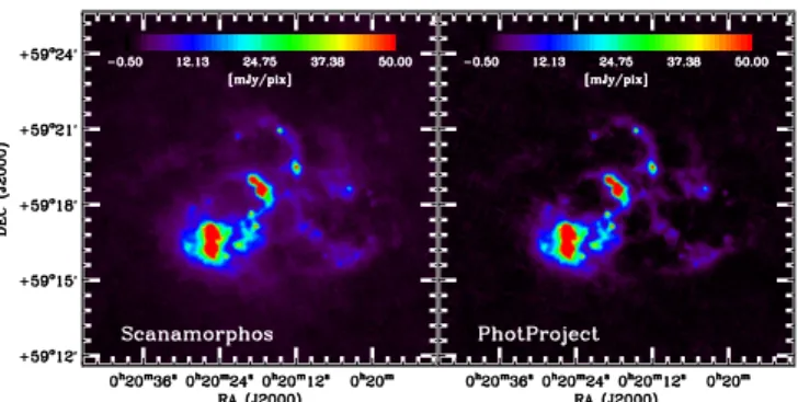
Fig. 2.S (left) and PP (right) images of IC 10 at 70 µm to illustrate how PP tends to clip out the extended features. The colours and spatial scales are the same on both images. Here the diffuse extended emission is best visible on the S map. The comparison of the total flux densities coming from the 2 meth-ods confirms that PP misses the extended emission: in this case, F70(S)/F70(PP) = 1.5.
of a flat background made for the photometry (see Sect.3.1.1). To avoid this problem, we decide to use the S maps for the extended sources.
2.2.3. SPIRE data reduction
Following the same method as in Ciesla et al.(2012) for the Herschel Reference Survey, or in Auld et al. (2013) for the HErschel VIrgo Cluster Survey, the SPIRE maps are processed through HIPE5using a modified version of the available SPIRE pipeline. The steps from the Level 0 to Level 1 are basically the same as in the official version provided by the SPIRE Instrument Control Centre (ICC). The pipeline starts with a first deglitching step, then a time response correction is applied to match the de-tector timelines to the astronomical pointing timelines. A second deglitching step is then performed as it improves the removal of residual glitches. After, an additional time response correction, the flux calibration step is performed, where non-linearity cor-rections are taken into account. An additional correction is ap-plied to the bolometre timelines to account for the fact that there is a delay in the response of the bolometres to the incoming sig-nal. The temperature drifts of the bolometres are then removed. For this step, the pipeline temperature drift removal is not run, instead a custom temperature drift correction (BGAE, Smith et al., in prep) is applied to the whole observation timeline (rather than an individual scan-leg). Finally, the N is used to construct the final map with pixel sizes of 6, 8, 1200for the 250,
350, 500 µm band respectively. For galaxies with heavy cir-rus contamination an additional destriping step is performed. A complete description of the data processing step will be given in Smith et al. (in prep.).
3. Photometry measurements for the DGS sample
In this section, we describe how we obtain the different PACS and SPIRE flux densities, together with their uncertainties, for the DGS sample (Tables2and3, Sects.3.1and3.2). The PACS flux densities are then compared with the existing MIPS flux densities (Sect.3.3).
3.1. PACS photometry 3.1.1. Extracting the fluxes
For PACS measurements, we perform aperture photometry, plac-ing an aperture on the source and a background region to esti-mate the sky level. Using the version 7 of the PACS photometric calibration available in HIPE, the point spread functions (PSFs) have been measured out to 100000. Most of our maps are smaller than this, which means, in principle, that some contribution from the PSF of the source can basically be found everywhere on the map, and, any emission from the source falling in the back-ground region must be taken into account when estimating the total source flux density.
Taking this aperture correction into account, aperture pho-tometry is performed, using circular apertures of 1.5 times the optical radius whenever possible. For cases where it is not, we adjust our apertures to be sure to encompass all the FIR emis-sion of the galaxy (Table 2). There are three special cases. For HS 0052+2536 the chosen aperture also encompasses the neigh-bouring very faint galaxy HS 0052+2537. Mrk 1089 is a galaxy within a compact group of galaxies and UM 311 is part of an-other galaxy and the chosen apertures encompass the whole group of objects. For these galaxies, the spatial resolution of the SPIRE bands makes it very difficult, if not impossible, to sepa-rate them from the other objects in their respective groups. For these few cases, the entire group is considered and is noted in Tables1−3. The background region is a circular annulus around the source. In most cases, the inner radius of the background region is the same as that of the source aperture and the outer radius is about two times the source aperture radius.
The maps are assumed to consist of the sum of a constant, flat background plus the contribution from the source. Flux den-sities are measured in the aperture ( fap) and in the background
annulus ( fbg) by summing the pixels in both regions. The
contri-bution to the measured flux densities ( fapand fbg) from the total
flux density of the galaxy ( ftot) and from the background (b) is
determined for each aperture using the encircled energy frac-tion (eef) tables. These tables, given by HIPE, are measurements of the fraction of the total flux density contained in a given aper-ture on the PSFs (inverse of the aperaper-ture correction). This gives us a simple linear system of two equations with two unknowns: the total flux density from the galaxy ( ftot) and the background
level (b):
( fap = ftot· eefr0+ Nap· b
fbg = ftot· (eefr2− eefr1)+ Nbg· b
(1)
where r0, r1, r2are the source aperture radius and the background
annulus radii respectively, and eefr0, eefr1and eefr2are the
encir-cled energy fractions at radii r0, r1, r2. Nap(resp. Nbg) is the
num-ber of pixels in the source (resp. background) aperture. Inverting this system gives us the values for ftotand b.
If one considers that there is no contribution from the source outside the source aperture, i.e. setting eefr0 = 1 and eefr1 =
eefr2 = 0, the flux density will be underestimated, as some con-tribution from the source will have been removed during the background subtraction. This underestimation depends on the source aperture size r0and can be important for small apertures.
The error made on the flux density becomes greater than the cali-bration error, which is the dominant source of uncertainty (∼5%, see Sect. 3.1.2), when r0 . 10. Given that the median r0 in the
DGS sample is ∼0.60, it is thus important to take the contribution from the source falling outside the source aperture into account.
3.1.2. Computing the uncertainties
The uncertainties on the flux density arise from the non-systematic errors due to the measurement of the flux density on the maps, (uncftot), and the systematic errors due to
calibra-tion, (unccalib).
For the measurement on the maps, the system of equations being linear, the uncertainties arising from the two measure-ments on the map (uncapand uncbg) can be linearly propagated
to the total flux density and the background level, giving us the uncertainty on the total flux density (uncftot) and the uncertainty
on the background level (uncb). The determination of uncap
and uncbgis the same for both errors as the measure is the same:
summing pixels in a given region of the map. Thus we detail the calculation for uncaponly.
There are two sources of errors to uncap: one coming from
the sum of the pixels, uncsum, one coming from the intrinsic error
on the flux density value in each pixel, uncint.
Determination of uncsum: for each pixel there is a contribution
from the background noise to the total measured flux density. This error, σsky, is the same for a pixel in the source aperture
as well as in the background aperture, repeated Naptimes here.
The error, σsky, is the standard deviation of all pixels in the
back-ground aperture. The final uncertainty, uncsum, is then:
uncsum = pNapσsky. (2)
Determination of uncint: for each pixel there is an underlying
un-certainty for the flux density value in the pixel, σint,i, and is
inde-pendent from pixel to pixel. This uncertainty arises from the data reduction step when the flux density for each pixel is computed. A map of these uncertainties is produced during the data reduc-tion process. The uncertainty, uncint, is then derived by adding
quadratically all of the errors in the considered pixels:
uncint= v u tNap X i= 0 σ2 int,i. (3)
Note that the assumption of pixel-to-pixel independent uncer-tainty is not applicable for PACS maps and this can result in an underestimation of uncint.
The total error on the source aperture measurement is then: uncap=
q unc2
sum+ unc2int. (4)
The uncbg is derived the same way and we can then compute
uncftot and uncb. The quantity uncftot is thus the total error on
the flux density due to measurement on the map. To this certainty, we add in quadrature the systematic calibration un-certainty, unccalib, of 5% for the three PACS bands (Sauvage &
Müller, priv. comm.), giving, in the end, the σ70−100−160reported
in Table2: σλ= q unc2 ftot+ unc 2 calib. (5)
Note that in uncsum, we have a combination of uncertainties from
small scale astronomical noise and instrumental uncertainties. These instrumental uncertainties can be redundant with part of the instrumental uncertainties taken into account in uncint,
lead-ing to an overestimate of uncapand thus uncftot. However, it has
a minor impact on the final uncertainties, σ70−100−160, as the
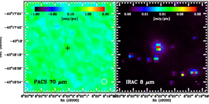
Fig. 3.Example of a PACS non-detection: (left) PACS 70 µm image of Tol 0618-402. The position of the galaxy is marked with a black cross. The IRAC 8 µm image has been added on the right for comparison. The PACS 70 µm (FWHM = 5.600
) and the IRAC 8 µm (FWHM = 2.000
) beams are indicated as white circles on the bottom right of the images.
3.1.3. Case of upper limits
Some galaxies in our sample are not detected in some or all of the PACS bands. We classify these galaxies as “upper limits” when the computed flux density is lower than five times the cor-responding uncertainty on the flux density (e.g. Tol 0618-402, Fig. 3). We take as the final upper limit, five times the uncer-tainty on the flux density value in order to have a 5σ upper limit (reported in Table2).
3.2. SPIRE photometry
For the SPIRE photometre, the relative spectral response func-tion (RSRF) is different for a point source or for an extended source. During the treatment by the pipeline, the measured RSRF-weighted flux density is converted to a monochromatic flux density for a source where ν*Fν is constant, via the “K4”
correction defined in the SPIRE Observers’ Manual (Sect. 5.2.7), assuming a point-like source. The output of the pipeline will be, by definition, a monochromatic flux density of a point source. To obtain monochromatic flux densities of extended sources we apply the ratio of K4 corrections for extended and
point-like sources, K4e/K4p, defined in the SPIRE Observers’
Manual (Sect. 5.2.7). In order to determine which sources need this extra-correction, we have to distinguish between extended and point-like (unresolved) sources in our sample, as well as non-detected sources. Extended sources are defined as galaxies whose spatial extension is larger than the FWHM of the SPIRE beam, and non-detected sources are galaxies that are not visible at SPIRE wavelengths.
3.2.1. Extracting the fluxes
The photometry method is adapted for each type of galaxy. However, as the data reduction has been performed with HIPE v5, the 350 µm maps are first scaled by a factor of 1.0067 to update the maps to the latest version of the 350 µm flux calibration (SPIRE Observers’ Manual (Sect. 5.2.8)).
Point source photometry
To determine the flux densities of point sources, we fit a Gaussian function (which is representative of the shape of the PSF) to the timeline data from the bolometres, using a timeline-based source fitter that is used for deriving the flux calibration
for the individual bolometres6. We then check a posteriori that our “unresolved” classification was correct: if the FWHM of the fitted Gaussian is <2000, 2900 and 3700 at 250, 350 and 500 µm respectively, then the source can be considered as truly point-like. As the timeline data is in Jy beam−1, the flux density will simply be the amplitude of the fitted Gaussian. This is the most accurate way of computing flux densities for point-like sources as it matches the measurement techniques used for the SPIRE calibration. Moreover we avoid all pixelization issues when using the timeline data rather than the map. On top of that, applying any mapmaking process would also smear the PSFs, causing the peak signal values to decrease by ∼5% for point sources.
Extended source photometry
For the extended sources, we perform aperture photome-try on the maps, using the same source and background aper-tures as those used for the PACS photometry, and check that the PACS apertures do fully encompass the SPIRE emission from the entire galaxy. The maps are converted from Jy beam−1 to
Jy pix−1considering that the beam area values are 465, 822 and 1768 square arcseconds7 at 250, 350, 500 µm respectively and
the pixel sizes are given in Sect.2.2.3.
The background level is determined by the median of all of the pixels in the background aperture. The median is pre-ferred rather than the mean because the SPIRE background is contaminated by prolific background sources due to some ob-servations reaching the confusion limit. The background level is then subtracted from our maps and the total flux density is the sum of all of the pixels encompassed in the source aperture, corrected for K4e/K4p. These K4e/K4p correction factors, given
in the SPIRE Observers’ Manual (Sect. 5.2.8), are 0.98279, 0.98344 and 0.97099 at 250, 350, 500 µm respectively.
However there are also “marginally” extended sources (e.g. II Zw 40) that do not require this K4e/K4pcorrection. To identify
these sources, we first check that the source is truly resolved by applying the point source method on the timeline data. We verify that the FWHM is indeed greater than the chosen threshold val-ues for the “unresolved” classification. As an additional check, the fitted Gaussian is subtracted from the map and the resulting map is visually checked for any remaining emission from the source. If this condition is satisfied, then the source is truly re-solved. If the FWHM of the fitted Gaussian is lower than 2400, 3400 and 4500 at 250, 350, 500 µm respectively then the source
is considered to be “marginally” extended only, and thus to not require the K4e/K4pcorrection.
3.2.2. Computing the uncertainties
As for the PACS photometry, there are two types of uncertainties for SPIRE photometry: the errors arising from the determination of the flux density, uncflux, and the calibration errors, unccalib.
As we used different methods for flux extraction depending on the type of the source, the errors contributing to uncflux are
determined differently. The method described here has been adapted from the method described inCiesla et al.(2012).
6 The last version of this source fitter is incorporated into HIPE v10
(Bendo et al., in prep.).
7 SPIRE photometre reference spectrum values:
http://herschel.esac.esa.int/twiki/bin/view/Public/ SpirePhotometerBeamProfileAnalysis, September 2012 values.
Point source photometry
The uncertainty on the flux density for a point source is de-termined through a test in which we add 100 artificial sources with the same flux density as the original source. They are added at random locations in the map, within a 0.3 deg box centred on the original source. The same photometry procedure was applied to the artificial sources and the final uncertainty is the standard deviation in the flux densities derived for the artificial sources. We quote the following uncertainties (uncflux) for
point-like sources:
– 6 mJy at 250 µm;
– 7 mJy (for flux densities >50 mJy) and 10 mJy (for flux den-sities.50 mJy) at 350 µm;
– 9 mJy at 500 µm. Extended source photometry
For the aperture photometry performed on the extended sources, we have four types of uncertainties contributing to uncflux: the uncertainty arising from the background level
de-termination, uncbg, the uncertainty due to background noise in
the source aperture, uncsource, the underlying uncertainty for the
flux density value in the pixel coming from the data reduction, uncint, and the uncertainty in the beam area value: uncbeam, which
is given to be 4%8.
The determination of the background level generates an un-certainty which will affect each pixel in the source aperture when subtracting the background level from the map. The uncertainty on the background level is uncbglevel = σsky/ pNbg, with σsky
be-ing here again the standard deviation of all of the pixels in the background aperture. This will affect the determination of the flux density for each pixel summed in the aperture:
uncbg= Napuncbglevel. (6)
The uncertainty due to background noise in the source aperture, uncsource, is determined the same way as the PACS uncap since
it is the uncertainty arising from summing the pixels in a given aperture:
uncsource= pNapσsky. (7)
The uncertainty arising from the underlying uncertainties of the flux density value in each pixel is computed the same way as for PACS. Here again, this uncertainty arises from the data reduction step when the flux density for each pixel is computed, and the pipeline produces the corresponding error map:
uncint= v u tNap X i= 0 σ2 int,i. (8)
The total uncertainty coming from the determination of the flux density for an extended source, is then:
uncflux=
q unc2
bg+ unc 2
source+ unc2int+ unc2beam. (9)
For both types of sources, we also add calibration uncertainties to uncflux to get the final total uncertainty. There are two
dif-ferent SPIRE calibration uncertainties: a systematic uncertainty of ∼5% coming from the models used for Neptune, the primary
8 This value is given in:http://herschel.esac.esa.int/twiki/
bin/view/Public/SpirePhotometerBeamProfileAnalysis
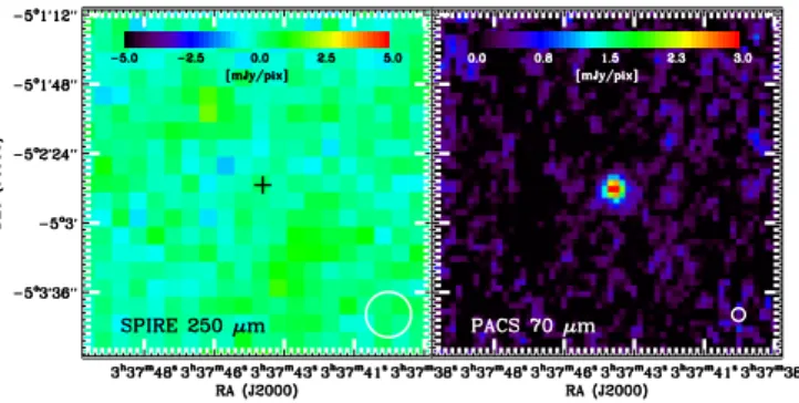
Fig. 4.Example of a SPIRE non detection: (left) SPIRE 250 µm and (right) PACS 70 µm image of SBS 0335-052. The position of the galaxy is indicated by a black cross on the SPIRE image. The SPIRE 250 µm (FWHM = 18.200
) and the PACS 70 µm (FWHM = 5.600
) beams are indicated as white circles on the bottom right of the images.
calibrator, which is correlated between the three bands, and a random uncertainty of ∼2% coming from the repetitive mea-surement of the flux densities of Neptune. These two uncertain-ties were added linearly instead of in quadrature as advised in the SPIRE Observer’s Manual, giving an overall 7% calibration uncertainty unccalib. The final total uncertainty, σ250−350−500
re-ported in Table3, is obtained by adding uncflux and unccalib in
quadrature.
As for PACS, with SPIRE we also have a redundancy in the error estimation in uncsourceand uncint, again with only a minor
impact on the final uncertainties, σ250−350−500, as the calibration
uncertainty dominates.
3.2.3. Case of upper limits
When the galaxy is not detected in the SPIRE bands (e.g.
SBS 0335-052, Fig. 4), we can only derive upper limits on
the flux density. Also, when the source is blended with another source in the beam and we are unable to confidently separate them (e.g. Pox 186 and a background galaxy separated by 2000,
Fig.5), upper limits are reported. Since the undetected sources are point sources, we use five times the uncertainties reported for point sources in3.2.2. The only exception is SBS 1533+574 which is blended with another source and slightly extended at 250 µm. The method described above gives an upper limit too low. The extended source photometry method is thus used to de-rive a 5σ upper limit at this wavelength.
3.2.4. Special cases: heavy cirrus contamination
For NGC 6822 and IC 10, the cirrus contamination from our Galaxy is important in the SPIRE bands.
NGC 6822 −Galametz et al.(2010) determined that the con-tribution from the cirrus to the total emission of the galaxy is of the order of 30% for all SPIRE bands. To determine the cirrus contribution here, we assume that the entire galaxy is in a homo-geneous and flat cirrus region. We determine this cirrus level by considering regions at the same cirrus level outside of the galaxy. This level is used as the background level for the flux determina-tion. We then compare this flux density with the flux density ob-tained when we consider an uncontaminated background region and get the contamination from the cirrus. We also find that the contribution of the cirrus to the total flux densities is about 30%, which is coherent with the results fromGalametz et al.(2010). Thus for this galaxy, the flux densities cited in Table3are flux densities where the cirrus contribution has been subtracted. We
Fig. 5.Example of a “mixed” source. SPIRE 500 µm (left) and PACS 160 (right) images of Pox186 and a contaminating background source. The sources are 2000
apart, and are well separated at 160 µm, but are completely blended at SPIRE 500 µm resolution. Pox 186 corresponds to the bottom cross, whereas the contaminating background source is the X. The SPIRE 500 µm (FWHM = 36.300
) and the PACS 160 µm (FWHM = 11.300
) beams are indicated as white circles on the bottom right of the images.
also include a conservative 30% uncertainty in the error for these flux densities to account for the estimation of the cirrus contri-bution, and for the fact that the cirrus emission may not be flat.
IC 10 −we apply the same method here. Again, we find that the cirrus contributes ∼30% on average, to each SPIRE band. We took this contribution into account by adding this cirrus uncer-tainty to the other sources of uncertainties for this galaxy.
This method can be improved, by using the HI maps to better determine the cirrus emission and the background level and thus reducing the uncertainties on the measurements for these two galaxies.
3.3. Comparison of PACS and MIPS existing flux densities We compare our PACS flux densities to the flux densities at 70 and 160 µm from MIPS onboard the Spitzer Space Telescope from Bendo et al.(2012) to assess the reliability of our measurements.
3.3.1. MIPS photometry
The table of the available MIPS data for the DGS is given in
Madden et al.(2013) andBendo et al.(2012) who give a detailed description of the photometry for total galaxy flux densities. Of the DGS sample, 34 galaxies have been observed by MIPS in the considered bands.Bendo et al.(2012) MIPS flux densities compare well with previously published MIPS samples contain-ing a subset of the DGS galaxies (Dale et al. 2007;Engelbracht et al. 2008). Therefore we are confident about the reliability of these results and will use them to perform the comparison with our PACS flux densities.
3.3.2. Comparison with PACS
The PACS flux densities correspond to monochromatic values for sources with spectra where ν fν is constant, while the MIPS
flux densities are monochromatic values for sources with the spectra of a 104 K blackbody, so colour corrections need to
be applied to measurements from both instruments before they are compared to each other. We first fit a blackbody through the three PACS data points and apply the corresponding colour
corrections from the available PACS documentation9. For the MIPS flux densities, we fit a blackbody through the 70 and 160 µm data points (not using the 24 µm point) and apply the corrections from the MIPS Handbook10. The typical colour
cor-rections for MIPS are of the order of 10 and 4% on average at 70 and 160 µm. However, they are of the order of 1 or 2% in the 70 and 160 µm PACS bands. For non-detected galaxies, where we, for PACS, and/orBendo et al.(2012), for MIPS, reported upper limits (nine galaxies), we are not able to properly fit a blackbody and therefore derive a proper colour correction. We do not com-pare PACS and MIPS flux densities for these galaxies for now.
We use the ratios of the PACS and MIPS flux densities to assess how well the measurements from the instrument agree with each other; a ratio of one corresponds to a very good agree-ment. The average PACS/MIPS ratios at 70 and 160 microns are shown in Fig.6, and the correspondence is relatively good. The PACS/MIPS ratio is 1.019 ± 0.112 at 70 µm and 0.995 ± 0.153 at 160 µm. This is to be compared to an average uncertainty of ∼12% (∼11% from MIPS and ∼5% for PACS, added in quadrature) and ∼16% (∼15% from MIPS and ∼7% for PACS, added in quadrature) on the ratios at 70 and 160 µm respec-tively.Aniano et al.(2012) found a slightly less good agreement (∼20%) for integrated fluxes of two KINGFISH galaxies.
If we now consider galaxies detected at 70 µm and not at 160 µm, indicated by a different symbol on the upper panel of Fig.6, we are still able to compare, with extra caution, the measurements at 70 µm. Indeed, as we are not able to derive a proper colour correction for those galaxies, we add to the MIPS 70 µm flux densities a 10% uncertainty and a 1% un-certainty to the PACS 70 µm flux densities to account for the colour correction effect. When adding these extra galaxies at 70 µm, the PACS/MIPS ratio is 0.985 ± 0.158 at 70 µm. This is to be compared with an average uncertainty of ∼14% on the 70 µm ratio (∼12% from MIPS and ∼7% for PACS, added in quadrature, including the extra galaxies). The very faint and dis-crepant galaxies at 70 µm are HS 1222+3741 (ratio of 0.40) and Tol 1214-277 (ratio of 0.24). For HS 1222+3741, the MIPS image contains some bright pixels near the edge of the pho-tometry aperture used for MIPS, and this may have driven the 70 µm MIPS flux density up. For Tol 1214-277, a nearby source is present in the MIPS data and, although its contribution has been subtracted when computing the MIPS 70 µm flux, some contribution from this source may still be present. Additionally, measuring accurate flux densities at ≤50 mJy in both MIPS and PACS data is difficult and may have led to the discrepancies.
The error on the average ratio is comparable to the average uncertainties on the ratio for both bands. Thus there is a good photometric agreement between PACS and MIPS photometry for the DGS sample.
4. Far Infrared and submillimetre behaviour and dust properties of the dwarf galaxies
To study the dust properties of the DGS and determine the im-pact of metallicity, we perform a comparison with galaxies from the KINGFISH sample (Kennicutt et al. 2011). The KINGFISH survey contains 61 galaxies: 41 spiral galaxies, 11 early-type
9 The corresponding documentation for PACS colour
correc-tions is available athttp://herschel.esac.esa.int/twiki/pub/ Public/PacsCalibrationWeb/cc_report_v1.pdf
10 The MIPS Instrument Handbook is available at http:
//irsa.ipac.caltech.edu/data/SPITZER/docs/mips/ mipsinstrumenthandbook/home/
Fig. 6. Comparison of PACS flux densities and MIPS flux densities: PACS-to-MIPS flux density ratios as a function of PACS flux density at 70 µm (top) and 160 µm (bottom). As a guide to the eye, the unity line is added as a solid line as well as the average uncertainties on the ra-tio in both bands as dotted lines. These average uncertainties are ∼12% and ∼16% at 70 and 160 µm. Colours distinguish the selected mapping method.
galaxies (E and S0) and nine irregulars (Kennicutt et al. 2011). KINGFISH is a survey including more metal-rich galaxies and enables us to span a wider metallicity range, notably by filling up the high-metallicity end of the metallicity distribution (Fig. 7). The metallicities adopted here for the KINGFISH sample have been determined the same way as for the DGS inKennicutt et al.
(2011), using the method of Pilyugin & Thuan (2005)11. No errors for metallicities are given in Kennicutt et al. (2011) so we adopt a 0.1 dex error for the KINGFISH metallicities. The Herschel KINGFISH flux densities are taken fromDale et al.
(2012)12.
11 SeeMadden et al.(2013) for the DGS metallicity determination. The
KINGFISH metallicities are from Col. 9 from Table 1 ofKennicutt et al. (2011).
12 The KINGFISH SPIRE fluxes and corresponding uncertainties are
updated to match the latest SPIRE beam areas. The beam areas used in this paper were released in September 2012, after the publication of Dale et al.(2012) in January 2012.
Fig. 7.Metallicity distributions for both DGS (purple) and KINGFISH (orange) samples. Note how the high metallicity end is better covered by KINGFISH whereas the low-metallicity end is better covered by the DGS.
We use FIR colour−colour diagrams (Sect. 4.1) and modi-fied blackbody models (Sect.4.2) in order to derive some physi-cal dust parameters of the galaxies, such as the temperature (T), the emissivity index (β), the dust mass (Mdust) and the FIR
lumi-nosity (LFIR). In Sect.4.3, we then investigate the presence of a
possible submm excess in the galaxies. 4.1. Characterization of the SED shapes
In order to obtain a qualitative view of the FIR-to-submm be-haviour of the DGS sample, and to compare with the KINGFISH sample, we inspect the observed Herschel SEDs as well as sev-eral Herschel colour−colour diagrams combining both PACS and SPIRE observations.
4.1.1. Observed spectral energy distributions
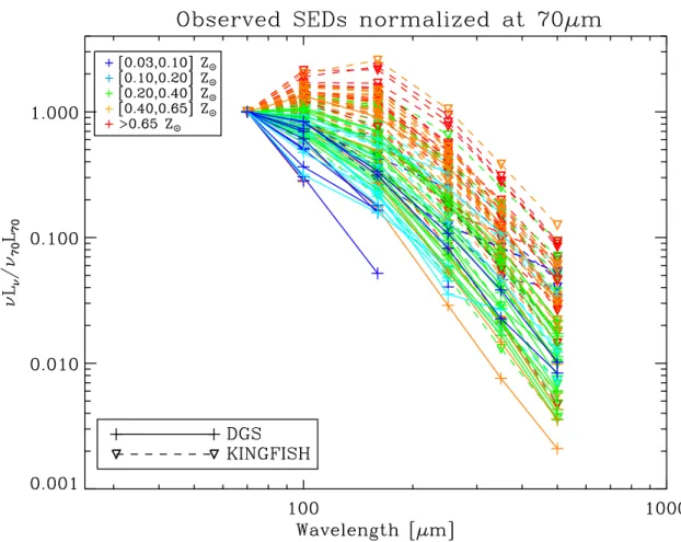
Total observed SEDs for both samples are computed for a first look at the characteristic SED shapes in the DGS and
KINGFISH samples (Fig. 8). The upper limits are not
in-dicated here for clarity. The most metal-poor galaxies are also the faintest and therefore not detected with Herschel be-yond 160 µm. The observed SEDs are normalized at 70 µm, and we see here that the peak of the SED shifts towards longer wavelengths as the metallicity increases, reflecting the impact of metallicity on the observed dust properties.
4.1.2. Dwarf Galaxy Survey colours Constructing the colour−colour diagrams
The Herschel colour−colour diagrams are constructed first by computing the observed ratios and the corresponding error bars, for both DGS and KINGFISH, and omitting the galaxies with more than one upper limit in the considered bands.
We then compute the theoretical Herschel flux ratios of sim-ulated modified blackbodies spanning a range in temperature (T from 0 to 40 K in 2 K bins and from 40 to 100 K in 10 K bins) and emissivity indices (β from 0.0 to 2.5). From now on, we define the emissivity index fixed for modelling the simulated Herschelflux ratios as “βtheo”, and “βobs” when we leave the
Fig. 8.Total Herschel observed SEDs for both DGS and KINGFISH samples, normalized at 70 µm. The colours delineate the different metallicity bins, and the lines and symbols differentiate DGS (plain lines and crosses) and KINGFISH galaxies (dashed lines and downward triangles).
emissivity index as a free parameter in modified blackbody fits (see Sect.4.2). In our simulated modified blackbody, the emitted fluxes are proportional to λ−βtheo× Bν(λ, T ), where Bν(λ, T ) is the
Planck function.
The pipeline we use for the data reduction gives us monochromatic flux densities for our data points for both PACS and SPIRE. To mimic the output of the pipeline for our theoretical points we weigh our theoretical flux density estimates by the RSRF of the corresponding bands. For SPIRE simulated measurements, we then convert our RSRF-weighted flux densities into monochromatic flux densities by applying the K4 correction given on the SPIRE Observers’ Manual. For
PACS, we also colour correct the RSRF-weighted modeled flux densities to a spectrum where νFν is constant (i.e. multiply by
the analogous of K4 for PACS). These simulated flux ratios
from a simple model are useful indicators to interpret the colour−colour diagrams.
FIR/submm colours
The spread of galaxies on the colour−colour diagrams (Figs.9and10) reflects broad variations in the SED shape and metallicity in our survey.
Indeed the DGS galaxies show a wider spread in location
on the diagrams compared to the KINGFISH galaxies (Figs.9
and10, top panels), reflecting the differences in the dust prop-erties between dwarf galaxies and the generally more metal-rich environments probed by the KINGFISH survey.
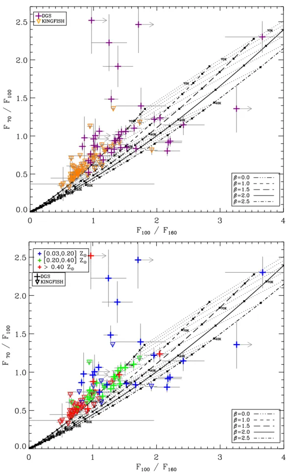
The F70/F100vs. F100/F160diagram (Fig.9) traces best the
peak of the SED. Galaxies usually exhibit a peak in their SED
around ∼100−160 µm. Galaxies presenting FIR flux densities with F70 > F100> F160may be quite warm as they peak at
wave-lengths less than 70 µm. Colder galaxies would lie in the lower left corner of the plot (F70< F100< F160), as shown by the
sim-ulated flux ratio lines. KINGFISH galaxies indeed cluster in the corresponding lower left corner of the plot while DGS galaxies span a wider space (Fig9, top). Nonetheless both samples follow the theoretical flux ratio lines from simulated modified black-bodies. There are some outliers, all of them being very faint, ex-tremely metal-poor galaxies (from 0.03 to 0.20 Z ). There is also
a metallicity trend in Fig.9(bottom), either between KINGFISH and the DGS or within both samples, i.e. low-metallicity (dwarf) galaxies peak at much shorter wavelengths and thus have over-ally warmer dust (several tens of K), compared to more metal-rich galaxies.
In dwarf galaxies, the warmer dust is due to the very en-ergetic environment in which the grains reside: the density of young stars causes the ISRF to be much harder on global scales than in normal galaxies (Madden et al. 2006). The low dust ex-tinction enables the FUV photons from the young stars to pen-etrate deeper into the ISM. The dust grains are thus exposed to harder and more intense ISRF than in a more metal-rich envi-ronment. This increases the contribution of hot and warm dust to the total dust emission resulting in overall higher equilibrium dust temperatures.
Note that there is a small excess at 70 µm for most of the galaxies compared to our simulated modified blackbodies, caus-ing them to fall above the lowest βtheo line. This means that if
we were to fit a modified blackbody only to the FIR flux den-sities (from 70 µm to 160 µm) we would get very low βobs, i.e.
Fig. 9. Colour−colour diagram: PACS/PACS diagram: F70/F100 versus F100/F160. Top: the colour and symbol code differentiates DGS (purple
crosses) and KINGFISH galaxies (orange downward triangles). Bottom: the colour code delineates the different metallicity bins this time. Crosses and downward triangles are still representing DGS and KINGFISH galaxies, respectively. For both plots, the curves give theoretical Herschel flux ratios for simulated modified black bodies for βtheo= 0.0 to 2.5 and T from 0 to 40 K in 2 K bins and from 40 to 100 K in 10 K bins, as black dots,
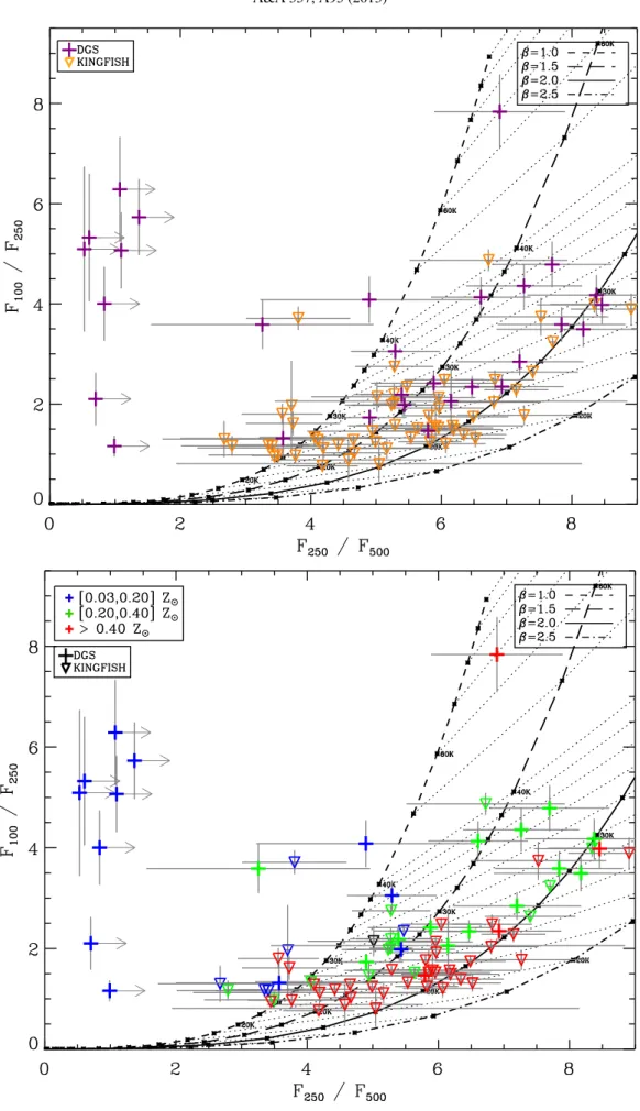
Fig. 10.Colour−colour diagram: PACS/SPIRE diagram: F100/F250versus F250/F500. The colour and symbol choices are the same as in Fig.9for
both figures. Note that the most metal-poor galaxies (from 0.03 to 0.20 Z ) are very faint and even not detected anymore at long wavelengths. We
a very flat SED in the FIR, which reflects a broad peak in the observed SED. This is due to the crudeness of the isothermal approximation made in the modified blackbody modelling. In a real galaxy, the dust grains are distributed in a range of tempera-tures, (e.g. hotter dust around star-forming regions vs colder dust in the diffuse ISM). Such a low βobshere is only a side effect of
the distribution in temperature of the grains in the galaxy. The extremely metal-poor outliers noted before may present an even wider temperature distribution than in more metal-rich galaxies, towards the higher temperatures, causing the broadening of the peak in their dust SED and their peculiar location on the dia-grams in Fig.9. Part of this excess at 70 µm could also be due to non-thermal heating, i.e. dust grains whose emission can not be represented by a modified blackbody, such as stochastically heated small grains.
More accurate values of T and βtheo may be illustrated
by including submm data in the colour−colour diagrams. At submm wavelengths (beyond ∼250 µm), the emissivity index this time represents an intrinsic grain property: the efficiency of the emission from the dust grain. A theoretical emissivity in-dex βtheo= 2 is commonly used to describe the submm SED for
local and distant galaxies in the models as it represents the in-trinsic optical properties of Galactic grains (mixture of graphite and silicate grains). More recently βtheobetween 1.5 and 2 have
also been used (e.g.Amblard et al. 2010; Dunne et al. 2011). The F100/F250 vs. F250/F500diagram (Fig.10) reflects best the
variations in emissivity index βtheo. Here again the DGS
galax-ies are more wide-spread than the KINGFISH galaxgalax-ies (Fig.10, top) spanning larger ranges of F100/F250and F250/F500ratios, that
is, wider ranges in temperature and β (such as higher T and lower β). As far as metallicity is concerned, the trend with tempera-ture already noted in Fig.9is still present (Fig.10, bottom). But hardly any trend between β and metallicity can be noticed: as the extremely low-metallicity galaxies are not detected at 500 µm, it is rather difficult to conclude on this point relying only on the
FIR/submm colour−colour diagram.
Modelling low-metallicity dwarf galaxies with grain prop-erties derived from the Galaxy (i.e. using βtheo = 2), may thus
not be accurate. The galaxies showing a lower βobs(βobs < 2)
will have a flatter submm slope. Smaller F250/F500 ratios, that
can be seen as a sign of lower βobs, indicative of a flatter submm
slope, have already been noted byBoselli et al.(2012) for sub-solar metallicity galaxies. This flatter slope may be the sign of a contribution from an extra emission in excess of the com-monly used βtheo= 2 models. Thus the flattening of the observed
submm slope (βobs< 2) could be used as a diagnosis for possible
excess emission appearing at 500 µm (see Sect.4.3).
4.2. FIR/submm modelling
To complete our observational and qualitative view of the FIR-submm behaviour of the DGS and KINGFISH galaxies, we use a modified blackbody model to quantitatively determine the parameters already discussed before: LFIR, Mdust, T, βobs, in the
DGS and KINGFISH samples.
4.2.1. Modified blackbody fitting
A single modified blackbody is fitted to the Herschel data of each galaxy from the DGS sample where the free parameters are: temperature (T) and dust mass (Mdust) as well as the emissivity
index (βobs), where we leave βobsfree in the [0.0, 2.5] range. The
modeled flux densities are given by:
Fν(λ)= Mdustκ(λ0) D2 λ λ0 !−βobs Bν(λ, T ) (10)
where κ(λ0) = 4.5 m2kg−1 is the dust mass absorption
opac-ity at the reference wavelength, λ0 = 100 µm. κ(λ0) has been
calculated from the grain properties ofZubko et al. (2004), as inGalliano et al.(2011)13, and is consistent with a βtheo = 2.
Leaving βobs to vary in our fit can produce lower dust masses
for lower βobs (Bianchi 2013). This effect is discussed for the
two dust masses relations we derive in Sect.4.2.3. Moreover, this particular choice for the value κ(λ0) will only affect the
ab-solute values of the dust masses. Choosing another model to derive κ(λ0) would not affect the intrinsic variations noted in
Sect.4.2.3. D is the distance to the source (given in Table1) and Bν(λ, T ) is the Planck function. Colour corrections are included
in the fitting procedure.
At 70 µm, possible contamination by dust grains that are not in thermal equilibrium, and whose emission cannot be repre-sented by a modified blackbody, can occur in galaxies. An ex-cess at 70 µm compared to a modified blackbody model can also appear, as seen in Fig.9, because dust grains in a galaxy are more likely to have a temperature distribution rather than a single temperature. For example in spiral galaxies (present in the KINGFISH sample), the dust emitted at 70−500 µm can originate from two components with different heating sources and potentially different temperatures (Bendo et al. 2010,2012;
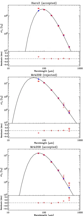
Boquien et al. 2011;Smith et al. 2012b). Therefore, we restrict our wavelength fitting range to 100−500 µm. The 70 µm point can be useful as an upper limit for a single temperature dust component. We redo the fit including the 70 µm point only if the modelled point from the fit without 70 µm data violates this upper limit condition, i.e. if it is greater than the observed point (e.g. Mrk 209 in Fig.11).
Some of our galaxies are not detected at some wavelengths. To have enough constraints for the fit, at least a detection up to 250 µm is required. If the galaxy is not detected beyond 160 µm, we fit a modified blackbody including the 70 µm point. Indeed some galaxies peaking at very short wavelengths have their Rayleigh Jeans contribution dropping at FIR and submm wavelengths, and are often not detected by SPIRE. For these galaxies, the 70 µm point is already on the Rayleigh Jeans side of the modified blackbody, and in this case we also include it in our fit.
All of these conditions are matched for 35 galaxies, and we use the 70 µm point for 11 of them (five because of the violation of the upper limit condition at 70 µm, four because the galaxy is not detected beyond 160 µm, and two because the galaxy is not observed by SPIRE, see Table4for details).
From the fitted modified blackbodies, we also derive the to-tal FIR luminosity, LFIR, by integrating the modelled curve
be-tween 50 and 650 µm. The resulting parameters from the fits are given in Table4. The SEDs are shown in Appendix A for all 35 DGS galaxies.
4.2.2. Rigorous error estimation
In order to derive conservative errors for our T, β, Mdust and
LFIR parameters we performed Monte Carlo iterations for each
fit, following the method in Galliano et al. (2011). For each
13 For their “Standard Model”, see Appendix A of Galliano et al.
Fig. 11.Examples of modified blackbody fits: the observed points are the red crosses whereas the modelled points are the filled blue circles. Upper limits are indicated with red diamonds. The bottom panel of each plot indicates the residuals from the fit. Top: fit for Haro 3, the observed 70 µm point which is not considered at first in our fitting pro-cedure, is above the modelled one. Centre: fit for Mrk 209. Here the observed 70 µm point is below the modelled one, and the fit should be redone, giving us: Bottom: fit for Mrk 209 using the 70 µm point. Note how the shape of the modified blackbody varies between the two: for example, the dust temperature for Mrk 209 goes from 56 K (with-out 70 µm) to 33 K (with 70 µm).
galaxy, we randomly perturb our fluxes within the errors bars and perform fits of the perturbed SEDs (300 for each galaxy). To be able to do this we must first carefully identify the various types of error and take special care for errors which are corre-lated between different bands.
As explained in Sects. 3.1.2 and 3.2.2, we have measure-ment errors and calibration errors in our error estimates. The measurement errors are independent from one band to another and are usually well represented by a Gaussian distribution. The calibration errors, however, are correlated between different bands as it is the error on the flux conversion factor. It can be summarized for our case as follow:
PACS: although the total calibration error is 5% in the three PACS bands it can be decomposed into two components:
– the uncertainty on the calibration model is 5% (according to the PACS photometre point-source flux calibration docu-mentation14) and is correlated between the three bands; – the uncertainties due to noise in the calibration observations
are: 1.4, 1.6, 3.5% at 70, 100, 160 µm, respectively (PACS photometre point-source flux calibration). These uncertain-ties are independent from one band to another.
SPIRE: the SPIRE ICC recommend using 7% in each band but here again we can decompose it:
– the uncertainty on the calibration model is 5% (SPIRE Observer’s Manual) and is correlated between the three bands;
– the uncertainties due to noise in the calibration observations are 2% for each band (SPIRE Observer’s Manual). These uncertainties are independent;
– As SPIRE maps are given in Jy beam−1, the error on the beam area will also affect the calibration. The uncertainty on the beam area is given to be 4% in each band15 and is independent.
The perturbation of the observed fluxes will then be the sum of two components:
– A normal random independent variable representing the measurement errors.
– A normal random variable describing the calibration errors that takes the correlation into account between the wave-bands as described above, the same for each galaxy. After performing 300 Monte-Carlo iterations, a distribution for each of the three model parameters T, β, Mdustas well as for LFIR
is obtained for each galaxy (see example on Fig.12). We chose to quote the 66.67% confidence level for our parameters defined by the range of the parameter values between 0.1667 and 0.8333 of the repartition function. As the distributions are often asym-metric we obtain asymasym-metric error bars on our parameters. These error bars are given in Table4.
4.2.3. FIR properties
We now have the T, β, Mdust and LFIRdistributions of the DGS.
We perform the same analysis for the KINGFISH sample in order to compare the distribution of parameters of the dwarf
14 http://herschel.esac.esa.int/twiki/bin/view/Public/
PacsCalibrationWeb?template=viewprint
15 This value is given in:http://herschel.esac.esa.int/twiki/