HAL Id: hal-01459103
https://hal.archives-ouvertes.fr/hal-01459103
Submitted on 26 Aug 2020
HAL is a multi-disciplinary open access archive for the deposit and dissemination of sci-entific research documents, whether they are pub-lished or not. The documents may come from teaching and research institutions in France or abroad, or from public or private research centers.
L’archive ouverte pluridisciplinaire HAL, est destinée au dépôt et à la diffusion de documents scientifiques de niveau recherche, publiés ou non, émanant des établissements d’enseignement et de recherche français ou étrangers, des laboratoires publics ou privés.
Wall surface temperature calculation in the
SolEdge2D-EIRENE transport code
J. Denis, B. Pégourié, J. Bucalossi, Hugo Bufferand, Guido Ciraolo, J-L
Gardarein, J. Gaspar, C. Grisolia, E. Hodille, M. Missirlian, et al.
To cite this version:
J. Denis, B. Pégourié, J. Bucalossi, Hugo Bufferand, Guido Ciraolo, et al.. Wall surface temperature calculation in the SolEdge2D-EIRENE transport code. Physica Scripta, IOP Publishing, 2016, 15th International Conference on Plasma-Facing Materials and Components for Fusion Applications, T167, �10.1088/0031-8949/T167/1/014073�. �hal-01459103�
This is the Accepted Manuscript version of an article accepted for publication in Physica Scripta. IOP Publishing Ltd is not responsible for any errors or omissions in this version of the manuscript or any version derived from it. The Version of Record is available online at
doi:10.1088/0031-8949/T167/1/014073.
Wall surface temperature calculation
in the SolEdge2D-EIRENE transport code
J. Denis1, B. Pégourié1, J. Bucalossi1, H. Bufferand2, G. Ciraolo1, J.-L. Gardarein3, J. Gaspar3, C. Grisolia1, E. Hodille1, M. Missirlian1, E. Serre4, P. Tamain1
1 CEA, IRFM, F-13108 Saint-Paul-lez-Durance, France
2 Aix-Marseille Université, CNRS, PIIM, UMR 7345, 13397 Marseille, France 3 Aix-Marseille Université, CNRS, IUSTI, UMR 7343, 13453 Marseille, France 4 Aix-Marseille Université, CNRS, M2P2, UMR 7340, 13451 Marseille, France
Email: [email protected]
Abstract
A thermal wall model is developed for the SolEdge2D-EIRENE edge transport code for calculating the surface temperature of the actively-cooled vessel components in interaction with the plasma. This is a first step towards a self-consistent evaluation of the recycling of particles, which depends on the wall surface temperature. The proposed thermal model is built to match both steady-state temperature and time constant of actively-cooled plasma facing components. A benchmark between this model and the Finite Element Modelling code CAST3M is performed in the case of an ITER–like monoblock. An example of application is presented for a SolEdge2D-EIRENE simulation of a medium-power discharge in the WEST tokamak, showing the steady-state wall temperature distribution and the temperature cycling due to an imposed Edge Localised Mode-like event.
1. Introduction
Among the most comprehensive tools used in global edge plasma modelling, 2D transport codes couple a 2D fluid description of the plasma to a kinetic module/code describing neutral species (atoms, molecules). These codes aim at incorporating as much physics as possible into neutrals, impurities and plasma wall interaction. In particular, the particle flux recycling on the Plasma Facing Components (PFCs) influences the edge properties through the nature of the reflected particles (atoms or molecules), their energy distribution and the generation of impurities [1]. The recycling properties vary with the PFC material, leading to significant difference – for instance – between carbon and full-metallic divertor operation [2,3]. The wall response (i.e. the recycling of particles) is also known to depend on the PFC surface temperature. In H-mode plasmas, this surface temperature varies as a function of space – due to the variable distance of the PFCs to the separatrix – and time – due to the periodic heat and particle pulses associated
with the Edge Localised Mode (ELM) activity [4]. This paper presents a time-dependent calculation of the wall temperature distribution designed for the SolEdge2D-EIRENE code package [5-8]. Indeed, this code is able to calculate the plasma characteristics up to the wall, in arbitrary tokamak geometry, and the incident flux distribution on the different PFCs is therefore accurately known. In the present paper, this calculation is performed and tested in post-processing. It will be completed by a wall model for a complete description of plasma wall interaction and of its consequence on the wall evolution (composition, erosion, migration, amount of retained particles) and plasma edge characteristics: a hydrogen absorption/desorption model will be implemented (e.g. [9]) and the coupling of SolEdge2D-EIRENE with an erosion/impurity migration code is foreseen (see, e.g. [10,11]). This fully-consistent code package will then be used to study the effect of ELM-like transient on the particles recycling (cf. [12] for a local calculation) and its impact on the divertor equilibrium.
The method for calculating the time-dependent wall temperature distribution is described in section 2 and its accuracy is tested in section 3. This calculation is then applied to the determination of the wall temperature in the WEST tokamak – briefly described in section 4 – under both a steady-state heat load and during an ELM-like event (section 5). The main results are summarised in section 6.
2. Surface temperature calculation of actively-cooled PFCs in the SolEdge2D-EIRENE transport code
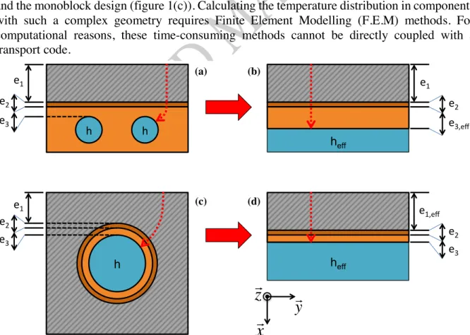
Operating a tokamak in steady-state requires actively-cooled PFCs, for which two technologies have been developed for the next generation of fusion devices: the flat tile design (figure 1(a)) and the monoblock design (figure 1(c)). Calculating the temperature distribution in components with such a complex geometry requires Finite Element Modelling (F.E.M) methods. For computational reasons, these time-consuming methods cannot be directly coupled with a transport code.
Figure 1: Flat tile (a) and monoblock (c) PFC designs with three material layers. Their corresponding representations in the wall model are displayed in (b) and (d). Typical heat flux lines are represented in red. The ith material layer thickness and the heat transfer coefficient between the heat sink and the coolant are defined as e
i heff e3# e1,eff# e2# h e3# e1# e2# heff e3,eff# e1# e2# h# h# e3# e1# e2#
x
y
z
(a) (c) (b) (d)and h, respectively. (en,eff, heff) refers to the couple of parameters adjusted in the model described in the present
paper.
To minimise the impact on the computation time of SolEdge2D-EIRENE, a simplified model was developed to calculate this temperature. In each cell intercepting the wall, a 1D radial time-dependent heat transfer calculation is used for determining this temperature. The complex geometry of the multi-material PFC is modeled by a superposition of layers (see figures 1(b) and (d)) separated by a contact resistance if required. The materials properties are assumed to be constant and uniform, thermal radiation is neglected1 and the lateral surfaces are considered insulated. The following heat equation is solved:
! 𝜕#𝑇 % 𝜕𝑥# = 𝜌%. 𝑐+,% 𝜆% 𝜕𝑇% 𝜕𝑡 𝑇%(𝑡 = 0, 𝑥) = 𝑇3 (1) 𝑄%(𝑥) = − 1 𝜆% 𝜕𝑇%(𝑥) 𝜕𝑥 (2)
where 𝑇%(𝑥) is the temperature and 𝑄%(𝑥) is the heat flux, both averaged over the (𝑦⃗, 𝑧⃗) directions (see figure 1). 𝜌%, 𝑐+,% and 𝜆% denote the 𝑖<= material density, specific heat capacity and conductivity, respectively.
Heat flux continuity is imposed at the interface between two materials layers and, if a contact resistance 𝑅 exists, an increase in temperature is induced according to (the index i increases with depth in the PFC):
𝑇% − 𝑇%?@ = 𝑅 × 𝑄% (3) For actively cooled PFCs, the boundary conditions are:
𝑄@(𝑡, 𝑥 = 0) = 𝑄%C (4)
𝑄%EFG(𝑡, 𝑥 = 𝑒<I<) = ℎK𝑇%EFG(𝑡, 𝑥 = 𝑒<I<) − 𝑇3L (5)
where 𝑒<I< is the overall thickness of the PFC (i.e. the coolant position), ℎ the heat transfer coefficient between the iMaxth layer in contact with the coolant (hereafter referred as the heat sink) and the coolant itself. 𝑇%EFG is the iMaxth layer temperature and 𝑇3 the coolant temperature. The system (1-5) is solved with the quadrupole method [13], allowing to calculate the surface temperature 𝑇NOPQ(𝑡) as a function of the incoming heat flux 𝑄%C(𝑡).
To ensure a correct thermal behaviour (i.e. to reproduce accurately the stationary surface temperature increase per MW, ∆SVTUFU
WX , and the heating/cooling time constant, 𝜏Z[\
2), the model has to take into account geometrical effects: in the complex PFC geometry, the heat flux lines between the surface and the coolant are curved and of variable length as illustrated in figures 1(a) and (c), which is not the case in a 1D model (see figures 1(b) and (d)). Moreover, in the PFC, the surface exposed to the plasma flux is not necessarily equal to the cooling pipe one (see figures 1(a) and (c)), whereas in a 1D model the two surfaces are equal by construction (see
1 This contribution is negligible: for a 10 MW.m-2 excitation of an ITER-like divertor monoblock, the surface
temperature is about 1000 °C and the radiation flux emitted by this surface is 0.06 MW.m-2. This also justifies the
fact that the lateral surfaces – which are only cooled by radiation – are assumed to be insulated.
2 Both determined either by laboratory measurements or by Finite Element Modelling (F.E.M., e.g. ANSYS or
figure 1(b) and (d)). To determine the PFC 1D equivalent geometry, the thickness of the layer where the coolant pipe is inserted 𝑒C (n being this layer number3) and the heat transfer coefficient ℎ are adapted, according to:
] ∆𝑇N<^< 𝑄%C = _ 𝑒% 𝜆% % +1 ℎ (6.1) 𝑇NOPQ(𝑡 = 3𝜏Z[\) = 95% 𝑇N<^< (6.2) where the relation linking ∆SVTUFU
WX , the material characteristics (𝑒%, 𝜆%) and the heat transfer coefficient ℎ results from the steady-state resolution of the system (1-5). The code is able to select, among all the couples of parameters strictly verifying relation (6.1), the one that better approximates relation (6.2). In the following, (𝑒C,dQQ, ℎdQQ) refers to this couple of adjusted parameters.
3. Model accuracy and comparison with F.E.M.
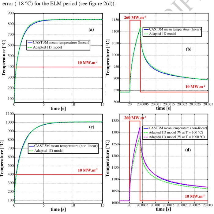
In the present exercise, a benchmark between F.E.M. code (taking into account the 2D PFC complex geometry) and the adjusted 1D model is achieved. The results from F.E.M. are taken as references to reproduce by the adjusted model. Two simulations are performed. In the first simulation, the mean surface temperature is calculated using the linear 2D heat equation (the materials properties are assumed to be constant and taken at 𝑇 = 100 °C). In the second one, the nonlinear 2D heat equation (the temperature dependence of material properties is taken into account) is used instead. Both simulations are performed with the F.E.M. code CAST3M [14]. An ITER-like monoblock of 30 mm in length and 29 mm in depth is considered. The layer 1, 2 and 3 (see figure 1(c)) are made of tungsten, copper and CuCrZr alloy, respectively. The material thicknesses (see figure 1(c)) are 𝑒@= 6 mm, 𝑒#= 1 mm and 𝑒h= 1.5 mm. The coolant temperature is 𝑇3 = 70 °C and the heat transfer coefficient is ℎ = 77940 W. mk#. °Ck@. The monoblock is submitted to a 10 MW.m-2 heat flux during 20 s to reach its steady-state. Then a substantial increase of the heat flux to 260 MW.m-2 during 400 µs is applied, followed by a return to a 10 MW.m-2 heat flux until 𝑡 = 20.02 ms. These load conditions are consistent with an ELM – inter-ELM cycle for a type I ELM, with an ELM frequency 𝜈nop = 50 Hz, an ELM duration 𝜏nop = 400 𝜇s and an ELM energy 𝑊nop = 100 kJ. mk#.
The results are displayed in figures 2(a) and (b) for the linear study and in figures 2(c) and 2(d) for the nonlinear one. Figures 2(a) and (c) show the step response to the 10 MW.m-2 heat flux. Figures 2(b) and (d) focus on the first three milliseconds of the ELM – inter-ELM cycle. The adjusting procedure is performed considering ∆SVTUFU
WX = 773 °C and 𝜏Z[\ = 1.00 s for the linear case and ∆SVTUFU
WX = 940 °C and 𝜏Z[\ = 1.44 s for the nonlinear one. In both cases the material properties are taken at 𝑇 = 100 °C. The procedure gives a couple w𝑒@,dQQ, ℎdQQx = (6.8 mm, 34700 W. mk#. °Ck@) for the linear case and w𝑒
@,dQQ, ℎdQQx = (9.5 mm, 33900 W. mk#. °Ck@) for the nonlinear one. This procedure enables the 1D model to be in good agreement with CAST3M for the linear simulation (see figure 2(a)), leading to a largest relative error of +1.7 % and a largest absolute error of +13 °C for the step response part. Concerning the ELM–inter-ELM cycle (see figure 2(b)), the largest relative error is +1.0 % and the largest
absolute error is +11 °C. Therefore, one can consider that the adjusted 1D model is able to rectify the geometrical effects that take place in the real monoblock. Concerning the non-linear simulation, the adjusting procedure is also able to compensate both the geometrical effects and the temperature dependence of materials properties (see figure 2(c) – the largest relative error is -3.5 % and the largest absolute error is -20 °C). However, during the ELM (see figure 2(d)), the 1D model underestimates the value of the temperature (-51 °C at the end of the ELM heat flux, which represents a relative error of -3.9 % on T and of -17 % on ΔT). Indeed, at the time scale of the ELM, the heat conduction into the first material is only driven by its thermal effusivity 𝐸@ = {𝜆@𝑐+,@𝜌@. Therefore, this error can be partially corrected by considering the first material (i.e. the tungsten) properties at 𝑇N<^< = 1000 °C. For this temperature, the new set of adjusted parameters is w𝑒@,dQQ, ℎdQQx = (6.0 mm, 31000 W. mk#. °Ck@). This new configuration leads to a lower relative error (-1.4 % on T and -5.9 % on ΔT) and a lower absolute error (-18 °C) for the ELM period (see figure 2(d)).
Figure 2: Comparison between the mean surface temperature of an ITER-like monoblock calculated with the Finite Element Modelling code CAST3M and the one calculated with the adjusted 1D model. An initial step response to a 10 MW.m-2 heat flux is applied (see (a) and (c)) until t = 20 s to ensure the steady-state to be reached in the
monoblock. Then an ELM is triggered during 400 μs, leading to an increase of the heat flux up to 260 MW.m-2. It
is followed by an inter-ELM period (see (b) and (d)). Comparisons are performed both with a linear CAST3M
0 5 10 15 100 200 300 400 500 600 700 800 900 time [s] T em p er at u re [
°C] CAST3M mean temperature (linear)Adapted 1D model
10 MW.m-2 (a) 0 5 10 15 100 200 300 400 500 600 700 800 900 1000 1100 time [s] T em p er at u re [
°C] CAST3M mean temperature (non-linear) Adapted 1D model 10 MW.m-2 (c) 20 20.0005 20.001 20.0015 20.002 20.0025 20.003 800 850 900 950 1000 1050 1100 1150 time [s] T em p er at u re [ °C]
CAST3M mean temperature (linear) Adapted 1D model (b) 10 MW.m-2 260 MW.m-2 20 20.0005 20.001 20.0015 20.002 20.0025 20.003 1000 1050 1100 1150 1200 1250 1300 1350 time [s] T em p er at u re [ °C]
CAST3M mean temperature (non-linear) Adapted 1D model (W at T = 100 °C) Adapted 1D model (W at T = 1000 °C)
10 MW.m-2 260 MW.m-2
simulation ((a) and (b)) and with a nonlinear one ((c) and (d)). The 1D thermal model is adjusted considering the materials properties at T = 100 °C. In figure (d), the 1D thermal model is also used considering the tungsten properties at T = 1000 °C, showing the importance of the first material layer in the surface temperature calculation during transients.
To summarize, handled in the right way, the 1D adjusted model is able to accurately reproduce PFCs behavior. For example, by considering the first material properties at the inter-ELM mean surface temperature, errors due to strong transient events can be lowered.
4. The WEST project
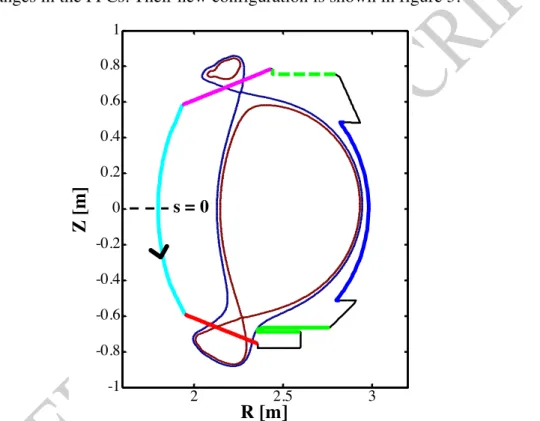
The WEST project consists in transforming Tore Supra in an X-point divertor configuration while extending its long pulse capability to test the ITER divertor components under combined heat and particle loads in a tokamak environment [15,16]. This transformation requires a number of changes in the PFCs. Their new configuration is shown in figure 3.
Figure 3: WEST main PFCs and wall geometry used in the SolEdge2D-EIRENE simulations: lower divertor (red, solid line); inner bumper (light blue, solid line); upper divertor (magenta, solid line); ripple and VDE protections (green, dashed line); stainless steel wall (black, solid line); antenna protection or outer limiter (dark blue, solid line) and baffle (green, solid line). The origin and direction of the s-coordinate along the wall are also displayed. The new set of PFCs consists in:
• The lower divertor, which follows the design and manufacturing processes foreseen for the ITER divertor elements: assembly of W monoblocks, high conductivity copper and copper alloy CuCrZr.
• The inner bumpers and outer limiter: flat W-coated carbon composite tiles attached to a copper alloy CuCrZr heat sink by means of a spring system.
• The upper divertor, based on a heat sink technology similar to the ITER first wall: assembly of copper alloy CuCrZr, high conductivity copper and stainless steel, with a tungsten coating instead of beryllium for ITER.
• The antenna protections: assembly of flat W-coated carbon composite tiles, high conductivity copper and copper alloy CuCrZr.
2 2.5 3 -1 -0.8 -0.6 -0.4 -0.2 0 0.2 0.4 0.6 0.8 1 R [m] Z [ m ] s = 0
• The lower divertor baffle and vacuum vessel protections against VDEs and ripple losses: set of W-coated copper alloy CuCrZr plates with cooling channels drilled inside. • The actively cooled stainless steel wall, featuring a “waver” structure [17].
The WEST PFCs 3D geometry has to be simplified and adapted to the 1D thermal model following the method described in section 2. The parameters to reproduce, ∆SVTUFU
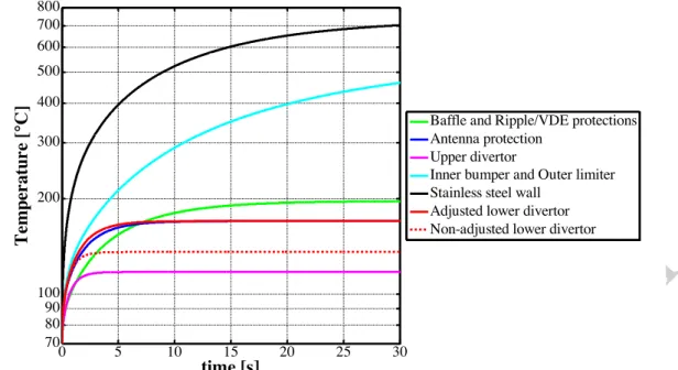
WX and 𝜏Z[\, are listed in table 1. The thermal time constants range between 2 and 20 s, showing that discharge durations of 40-60 s are required to reach a full steady-state over the whole vacuum vessel. The thicknesses 𝑒% and 𝑒C,dQQ (mm), and the effective heat transfer coefficients heff (W.m-2.°C-1), resulting from the procedure described in section 2, are also given. For each PFC, the effective thickness 𝑒C,dQQ is written with a bold font (other values 𝑒% are taken from the real PFC geometry). The considered cooling temperature is 𝑇3 = 70 °C.
Lower divertor Inner bumper Outer limiter Upper divertor Antenna protection Baffle VV protections SS wall ΔTstat/Qin (°C.W-1.m2) 1´10-4 5´10-4 4.8´10-5 1´10-4 1.3´10-4 6.6´10-4 τPFC (s) 2 20 1 2 5 10 ei (mm) W 8 => 11 15´10-3 15´10-3 15´10-3 15´10-3 - CFC - N11 - 20 - 6 - - Cu OFHC 1 2 - 1 - - CuCrZr 1.5 3 => 4 3 => 7 3 => 7 4 => 17 - SS 316 L - - - 2 => 8 heff (W.m-2.°C-1) 3.6´104 2.5´103 4.0´104 2.0´104 1.4´104 7.2´103 h (W.m-2.°C-1) 1´105 4´104 4´104 4´104 4´104 4´104
Table 1: Steady-state surface temperature increase per W.m-2, ∆STUFU
VWX , thermal time constant, 𝜏Z[\, materials thickness, 𝑒% and 𝑒C,dQQ, effective heat transfer coefficients, heff, of the WEST PFCs. The 𝑒C,dQQ values are written in bold. The heat transfer coefficient, h, resulting from F.E.M. simulations is given for comparison.
The WEST PFCs step responses to a heat flux 𝑄%C = 1 MW. mk# are displayed in figure 4. The colour code is the same as in figure 3. One can see the importance of adapting the PFC geometry (see section 2) by comparing the two red curves, which correspond to the lower divertor monoblock: using the couple (𝑒@, ℎ) instead of (𝑒@,dQQ, ℎdQQ) leads to a relative error of -65 % on 𝜏Z[\ and of -42 % on ∆SVTUFU
Figure 4: WEST PFCs step response to a heat flux Q~•= 1 MW. mk#. The colour code is the same as in figure 3. The red solid and dashed lines are the lower divertor calculated responses using the couples (e@,•‚‚, h•‚‚) and (e@, h), respectively.
5. Wall surface temperature distribution
In this section, the thermal wall model described in section 2 is applied to two different cases involving the WEST tokamak to show its abilities in both steady-state and transient heat loads.
5.1. Steady-state heat load
The temperature calculation was applied to a SolEdge2D-EIRENE simulation of a pure deuterium WEST discharge with a density at the separatrix 𝑛Nd+ = 2 × 10@… mkh, a power through the separatrix 𝑃Nd+ = 7.4 MW and a mid-plane heat flux e-folding length 𝜆VNd+,O+ = 7 mm. The integrated incident power on the different PFCs, 𝑃%C3, is listed in table 2.
Lower divertor Inner bumpers Outer limiter Upper divertor Antenna protection Baffle VV protection SS wall Pinc (MW) 5.3 0.3 0.8 0.1 0.7 0.2
Table 2: Incident power, 𝑃%C3, on the different WEST PFCs for a 7.4 MW WEST discharge.
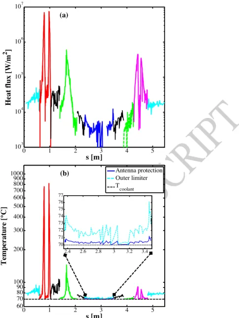
The space resolved incident net heat flux (including radiation and neutral contributions) and resulting wall temperature distribution are displayed in figure 5 (the definition of the wall coordinate s and colour code are explicated in figure 3).
0 5 10 15 20 25 30 70 80 90 100 200 300 400 500 600 700 800 T em p er at u re [ °C] time [s]
Baffle and Ripple/VDE protections Antenna protection
Upper divertor
Inner bumper and Outer limiter Stainless steel wall
Adjusted lower divertor Non-adjusted lower divertor
Figure 5: (a) Heat flux 𝑄%C and (b) surface temperature 𝑇N<^< distributions on the WEST PFCs. The definition of the wall coordinate s and the colour code are explicated in figure 3. The insert concentrates on the low field side of the vessel where the plasma is intercepted by the antenna protections or the outer limiter, depending on the toroidal location.
The heat flux reaches ~8 MW.m-2 on the lower divertor and ~1 MW.m-2 on the baffle and on the upper divertor. The surface temperature – assuming a flat surface, without shaping – remains lower than 200 °C everywhere, except on the lower divertor where it reaches ~820 °C. The discontinuities in the temperature distribution or differences for an almost identical heat load (e.g. the baffle and the upper divertor) are due to the differences in the heat removal capability of the different PFCs.
5.2. ELM-like transient
The power deposition during an ELM is roughly extrapolated from the steady-state profile calculated in the previous section. The energy expelled per ELM (∆𝑊nop) is given by ∆𝑊nop ≈ 𝛼. 𝑃Nd+/𝜈nop where 𝑃Nd+ denotes the power crossing the separatrix and 𝜈nop the ELM frequency. An empirical value for 𝛼 is typically 0.4 for Type I ELMs [18]. Considering an ELM duration 𝜏nop, the power load during an ELM is:
0 1 2 3 4 5 60 70 80 90 100 200 300 400 500 600 700 800 900 1000 s [m] T em p er at u re [ °C] Antenna protection Outer limiter Tcoolant 0 1 2 3 4 5 103 104 105 106 107 s [m] H eat f lu x [ W/ m 2 ] 2.4 2.6 2.8 3 3.2 3.4 70 71 72 73 74 75 76 77 (b) (a)
𝑃nop = ∆𝑊nop 𝜏nop =
𝛼. 𝑃Nd+
𝜏nop. 𝜈nop (7)
Only a fraction of this power (~60 %) impacts the divertor [19]. The wetted area is increased by a factor 𝜎nop ~ 1.3 − 1.4 w.r.t. the inter-ELM phase [20] and the asymmetry between the inner and outer divertor legs is set to 𝑟%:I ~ 2: 1 [21]. In the case of WEST, representative values are 𝜈nop ~ 50 Hz and 𝜏nop ~ 400 𝜇s. 𝑃Nd+ and 𝑄Ž%•dP<IP%C<dPknop are taken from the simulation of section 5.1.
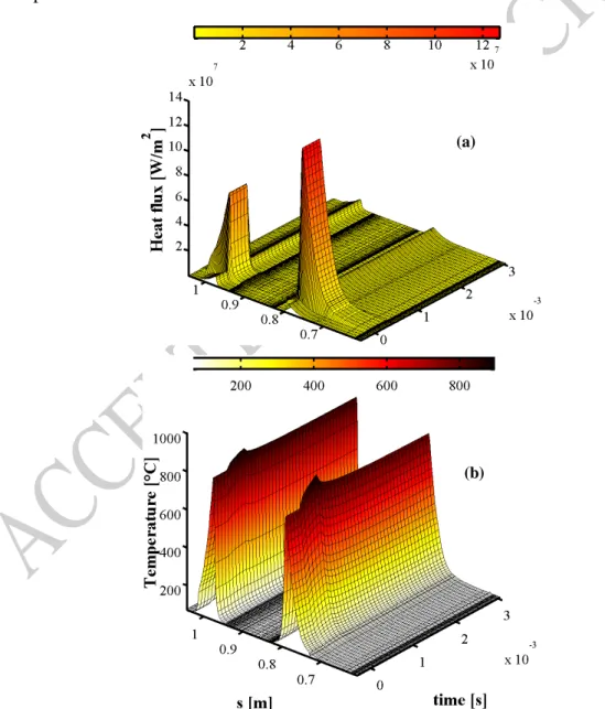
The result is shown in figure 6. In this figure, the s axis is oriented to highlight the inboard heat flux which is stronger during the ELM. Figure 6(a) displays the heat load during the ELM cycle. The ELM triggers at t = 0 s. In figure 6(b), the temperature profile is shown during the ELM cycle. The increase in temperature remains limited: ∆𝑇p^• ~ 130 °C. The surface temperature at the end of the ELM period is quasi-identical to the steady-state value, due to the fact that the ELM is short enough for the pulse heating to be essentially concentrated in a thin layer at the divertor plate surface.
Figure 6: (a) Heat load and (b) surface temperature distributions on the lower divertor during and in between ELMs. The ELM triggers at t = 0 s and lasts 400 µs. At the end of the ELM cycle (𝑡 = 𝑡nop+ 1 𝜈⁄ nop) the steady-state surface temperature is recovered.
(a)
6. Conclusion
A time-dependent calculation of the wall surface temperature distribution is designed for the SolEdge2D-EIRENE transport code. The heat transfer in actively-cooled PFCs is calculated in a 1D approximation using the thermal quadrupole method, with a procedure for reproducing accurately their thermal behaviour despite the simplification resulting from the choice of a 1D model. An example of application is presented for a medium-power discharge in the WEST tokamak, leading to the prediction of the steady-state temperature distribution in the whole vacuum vessel and to the transient increase of the lower divertor temperature during ELM cycling. This work will be completed soon by a wall model for a complete description of plasma wall interaction and of its consequence on the wall evolution and plasma edge characteristics.
Acknowledgements
This work was funded by the Provence-Alpes-Côte d’Azur Regional Council. It was granted access to the HPC resources of Aix-Marseille Université financed by the project Equip@Meso (ANR-10-EQPX-29-01) of the program “Investissement d’Avenir” supervised by the Agence Nationale pour la Recherche.
References
[1] Federici G. et al., Nucl. Fusion, 41, 1967 (2001)
[2] Brezinsek S. et al., J. Nucl. Mat., 463, 11 (2015) doi:10.1016/j.jnucmat.2014.12.007
[3] Schneider P.A. et al., Plasma Phys. Control. Fusion 57, 014029 (2015) [4] Marki J. et al., J. Nucl. Mat., 390–391, 801 (2009)
[5] Bufferand H. et al., Nucl. Fusion, 55, 053025 (2015) [6] Bufferand H. et al., J. Nucl. Mater. 415, S579 (2011) [7] Bufferand H. et al., J. Nucl. Mater. 438, S445 (2013)
[8] Serre E. et al., Contributions to Plasma Physics 52, 401 (2012
[9] Hodille E. et al., J. Nucl. Mat. (2015) doi:10.1016/j.jnucmat.2015.06.041
[10] Schmid K. et al., J. Nucl. Mat., 415, S284 (2011) [11] Schmid K., J. Nucl. Mat., 438, S484 (2013)
[12] Schmid K., Phys. Scripta, 15th International Conference on Plasma-Facing Materials and Components for Fusion Applications (2015)
[13] Maillet D. et al., Thermal Quadrupoles, Wiley & Sons, New-York (2000) [14] CEA, DEN, DM2S, SEMT, Cast3M, <http://www-cast3m.cea.fr/>. [15] Bucalossi J. et al., Fus. Eng. Des. 89, 907 (2014)
[16] Bourdelle C. et al., Nucl. Fusion 55, 063017 (2015) [17] Lipa M. et al., Fus. Eng. Des. 56-57, 855 (2001)
[18] Herrmann A., Plasma Phys. Contr. Fusion 44, 883 (2002) [19] Herrmann A. et al., Plasma Phys. Control. Fusion 46 (2004) [20] Eich T. et al., J. Nucl. Mat. 415, S856 (2011)