HAL Id: hal-02329380
https://hal.archives-ouvertes.fr/hal-02329380
Submitted on 24 Nov 2020
HAL is a multi-disciplinary open access
archive for the deposit and dissemination of
sci-entific research documents, whether they are
pub-lished or not. The documents may come from
teaching and research institutions in France or
abroad, or from public or private research centers.
L’archive ouverte pluridisciplinaire HAL, est
destinée au dépôt et à la diffusion de documents
scientifiques de niveau recherche, publiés ou non,
émanant des établissements d’enseignement et de
recherche français ou étrangers, des laboratoires
publics ou privés.
P. Kaaret, A. Zajczyk, D. Larocca, R. Ringuette, J. Bluem, W. Fuelberth, H.
Gulick, K. Jahoda, T. Johnson, D. Kirchner, et al.
To cite this version:
P. Kaaret, A. Zajczyk, D. Larocca, R. Ringuette, J. Bluem, et al.. HaloSat : A CubeSat to Study the
Hot Galactic Halo. The Astrophysical Journal, American Astronomical Society, 2019, 884 (2), pp.162.
�10.3847/1538-4357/ab4193�. �hal-02329380�
arXiv:1909.13822v2 [astro-ph.IM] 16 Oct 2019
HaloSat - A CubeSat to Study the Hot Galactic Halo
P. KAARET,1A. Z AJCZYK,1, 2, 3D. M. L AROCCA,1R. R INGUETTE,1 J. B LUEM,1W. F UELBERTH,1H. G ULICK,1K. J AHODA,2
T. E. JOHNSON,2D. L. KIRCHNER,1D. KOUTROUMPA,4K.D. KUNTZ,5R. MCCURDY,1 D. M. MILES,1 W. T. ROBISON,1 E. M. SILICH,1
1Department of Physics and Astronomy, University of Iowa, Iowa City, IA 52242, USA 2NASA Goddard Space Flight Center, Greenbelt, MD 20771, USA
3Department of Physics, University of Maryland, Baltimore County, 1000 Hilltop Circle, Baltimore, MD 21250 4LATMOS/IPSL, CNRS, UVSQ Universit´e Paris-Saclay, UPMC Univ. Paris 06, Guyancourt, France 5The Henry A. Rowland Department of Physics and Astronomy, Johns Hopkins University, Baltimore, MD 21218, USA
(Accepted September 3, 2019)
ABSTRACT
HaloSat is a small satellite (CubeSat) designed to map soft X-ray oxygen line emission across the sky in order to constrain the mass and spatial distribution of hot gas in the Milky Way. The goal of HaloSat is to help determine if hot gas gravitationally bound to individual galaxies makes a significant contribution to the cosmological baryon budget. HaloSat was deployed from the International Space Station in July 2018 and began routine science operations in October 2018. We describe the goals and design of the mission, the on-orbit performance of the science instrument, and initial observations.
Keywords:X-ray observatories (1819), Diffuse x-ray background (384), Circumgalactic medium (1879), Hot ionized medium (752), X-ray surveys (1824), Space vehicle instruments (1548)
1. INTRODUCTION
Astronomy at wavelengths that do not penetrate Earth’s at-mosphere requires space-borne observatories which tend to be costly, severely limiting their number. As of early 2018, there were only seven X-ray observatories in orbit as com-pared to the∼100 ground-based optical telescopes with aper-tures of 2 m or larger. The development of the CubeSat standard (Hevner et al. 2011) decoupled the design of small satellites from specific launch opportunities and has led to a large increase in the frequency of small satellite flights in-cluding frequent launch opportunities for scientific missions
(Crusan & Galcia 2019). The commercialization of small
satellite technologies has both increased the capabilities of small satellites and decreased their cost. Small spacecraft with the pointing accuracy, communications, and power re-sources needed for modest astronomical instruments can now be purchased at prices similar to that of a 1-m optical tele-scope. This enables low-cost, space-borne astronomical ob-servatories.
HaloSat is the first astrophysics-focused CubeSat mission funded by NASA’s Astrophysics Division. HaloSat’s scien-tific goal is to constrain the mass and spatial distribution of hot gas associated with the Milky Way by mapping soft X-ray
Corresponding author: Philip Kaaret
line emission from highly ionized oxygen in order to deter-mine if hot halos associated with individual galaxies make a significant contribution to the cosmological baryon budget. The mission was developed on a rapid time scale, less than 2.5 years from the start of funding to launch, and at modest cost, less than $4M. HaloSat was deployed from the Interna-tional Space Station (ISS) on 13 July 2018 and began routine science operations in October 2018.
In the following, we give an overview of the HaloSat mis-sion including the science goals and mismis-sion design in sec-tion2. We describe the science instrument in section3and the spacecraft and operations in section4. We present the on-orbit performance in section5. We discuss initial halo observations and plans for the survey in section6. Some of the text and figures in this paper have appeared previously in conference proceedings (Zajczyk et al. 2018;Kaaret et al.
2019).
2. MISSION OVERVIEW 2.1. Science Goals
Our Milky Way galaxy provides a local laboratory for un-derstanding the missing baryon problem. The total mass of the Milky Way has been dynamically measured to be(1.0 − 2.4) × 1012
M⊙ (Boylan-Kolchin et al. 2013). If the
cos-mological baryon fraction of 15.5% (Planck Collaboration 2014) applies on the scales of individual galaxies, then the Milky Way’s baryonic mass should be(1.6−3.7)×1011
M⊙. However, the observed baryonic mass in stars and disk gas is
only0.7 × 1011
M⊙ (McMillan 2011;Dame 1993). Thus,
more than half the expected baryons in the Milky Way are missing.
The presence of a hot Galactic halo has long been sus-pected (Spitzer 1956). Absorption lines at zero redshift in the X-ray spectra of extragalactic objects firmly estab-lish the existence of an extended distribution of hot gas, ∼106
K, associated with the Milky Way (Nicastro et al. 2002). Other evidence for a hot halo includes ubiquitous gas depletion in dwarf galaxies within 270 kpc of the Milky Way (Grcevich & Putnam 2009) understood as ram-pressure stripping and the dispersion measures of pulsars in globular clusters and the Magellanic clouds (Zhezher et al. 2017).
X-ray absorption line measurements of the halo are fea-sible along only about 30 lines of sight. In contrast, X-ray emission lines can be measured in any direction and provide a means to obtain a synoptic view of the halo gas. Data from existing X-ray observatories, primarily XMM-Newton and
Suzaku, have been used for emission line measurements of the halo (Smith et al. 2007;Yoshino et al. 2009;Henley et al.
2010; Henley & Shelton 2012; Miller & Bregman 2015).
However, the existing X-ray observatories are not designed for the efficient study of large-angular-scale diffuse emission and the spectra are often contaminated by heliospheric fore-ground emission that limits the accuracy of measurements of the halo (Slavin et al. 2013).
HaloSat’s scientific goal is to constrain the mass and spatial distribution of hot gas associated with the Milky Way. We chose to do this by measuring line emission from oxygen, the most cosmologically abundant element that is not fully ionized at the temperatures present in the halo. Oxygen in the halo is highly ionized and the strongest emission is in the soft X-ray range from the O VIItriplet near 574 eV and the pair of O VIIIlines near 654 eV. To advance over previous studies of halo oxygen line emission, we set an observational goal of achieving a 1σ statistical accuracy of±0.5 LU (LU = photons cm−2s−1ster−1) on the sum of the O VIIand OVIIIline emission in the 500-700 eV range for an oxygen line strength of 5 LU.
The Milky Way’s halo fills the entire sky. The observa-tional goal of HaloSat is to survey at least 75% of the sky with priority given to fields at Galactic latitudes|b| ≥ 30◦. Modest angular resolution of 15◦or less is sufficient to map the halo emission. HaloSat uses non-imaging detectors to minimize cost and complexity, hence the angular resolution is set by the field of view. We chose a large field of view with a10◦diameter full response dropping to zero response at a diameter of14◦, which is consistent with the required angular resolution.
2.2. Mission Design
We chose to implement HaloSat as a CubeSat. The largest CubeSats being regularly flown by NASA at the time of mis-sion formulation were in the 6U form factor with a volume of 8600 cm3
. Approximately one third of the volume was allocated to the spacecraft structure and systems leaving a volume of roughly 6000 cm3
available for the science
instru-ment. The choice of a CubeSat also limits the mission dura-tion. The most common launch for US-based CubeSats is to the ISS and the relatively low altitude,∼400 km limits the orbital lifetime. HaloSat’s orbital lifetime is expected to be 2.5 years. Furthermore, CubeSat electronics often use com-mercial rather than radiation hardened electronic components to minimize cost which can lead to premature failure in the space environment. HaloSat was designed with a baseline mission lifetime of 405 days based on the longest lifetimes achieved with similar components in previous missions.
HaloSat is designed to be sensitive to diffuse X-ray emis-sion. The number of oxygen line photons detected from a diffuse source is N= f AΩT , where f is the diffuse line flux generally measured in LU, A is the detector effective area at the oxygen line,Ω is the detector/telescope field of view, and T is the observation time. The figure of merit for observ-ing diffuse emission is AΩ or ‘grasp’. Due to the CubeSat volume constraints, HaloSat uses three small detectors that view the sky through mechanical collimators with no optics. Each detector has an effective area for X-rays of 600 eV of about 5.1 mm2
. However, HaloSat’s field of view is near 100 square degrees, enabling it to efficiently survey the sky. The total grasp of HaloSat at 600 eV is17.6 cm2
deg2
. The grasp of the Chandra X-ray Observatory at the same energy was about2× lower at launch, while the total grasp of the two
XMM-NewtonEPIC-MOS is about4× larger. Thus, a Cube-Sat can be competitive with major space observatories when designed for a specific goal, such as survey efficiency.
The accuracy of current emission line measurements of the halo is limited by foreground oxygen emission produced by solar-wind charge exchange (SWCX), when energetic parti-cles in the solar wind exchange charge with neutral atoms within the solar system (for a review, see Kuntz 2019). HaloSat observes towards the anti-Sun direction during the nighttime half of the 93-minute orbit of the spacecraft around Earth to minimize this foreground. This is not possible with
XMM-Newtonbecause it has a fixed solar array that restricts observations to a Sun angle range of 70◦-110◦. Because the solar system background presents the dominant uncertainty in current line intensity measurements, HaloSat has an addi-tional science goal to improve our understanding of SWCX emission and conducts observations specifically devoted to this goal.
2.3. Solar wind charge exchange emission
Solar wind charge exchange (SWCX) emission occurs when a highly charged ion of the solar wind interacts with a neutral atom and gains an electron. The resulting ion is in an excited state and may decay by emitting an X-ray. SWCX emission is produced within Earth’s magnetosheath and throughout the heliosphere. The line flux is the integral over the line of sight of the product of the ion density, the neutral density, the relative velocity between the ion and neu-tral, the charge exchange cross-section, and the line emission probability. The magnetosheath responds rapidly to changes in the solar wind flux, so its SWCX emission is strongly time-variable. The heliospheric emission is integrated over a long
line of sight, sampling about a month of solar wind condi-tions, and varies more slowly.
The distribution of heliospheric emission is determined by the geometry of the target gas. Neutral interstellar gas flows at∼ 25 km/s through the Solar System. This gas, mostly hydrogen but with∼ 15% helium, flows from the Galactic direction(l ∼ 3◦, b∼ 16◦), placing the Earth downstream of the Sun in early December. The flow of interstellar hydrogen is affected by both radiation pressure and gravity, and the hy-drogen becomes strongly ionized through charge exchange with solar protons and photo-ionization so that the hydrogen is denser upstream of the Sun than downstream. In contrast, the interstellar helium flow is not strongly ionized but is af-fected mainly by gravity, which focuses the flow downstream of the Sun into the ‘He-focusing cone’.
The heliospheric O VII and O VIII emission are calcu-lated from the interstellar neutral H and He distributions and measurements of the solar wind provided by solar and he-liospheric observatories (Koutroumpa et al. 2009). A crucial input to this modeling is knowledge of the O-He interac-tion cross secinterac-tion (Galeazzi et al. 2014). HaloSat observed along the focusing when the Earth passed through the He-focusing cone in December 2018 with observations made at roughly monthly intervals from two months before the pas-sage to two months after. By correlating the observed soft X-ray emission with the He distribution along the line of sight, these HaloSat observations will provide an accurate measure-ment of the O-He cross section and an absolute scale for the SWCX models. These observations cannot be done by any other current observatory.
HaloSat is also carrying out a series of observations to study magnetospheric SWCX emission. A selected set of tar-gets is observed multiple times, once near the anti-Sun direc-tion in order to minimize magnetospheric SWCX emission and also as the target enters and exits the anti-Sun hemisphere and is viewed through the flanks of the magnetosheath. These flank observations should have significant magnetospheric SWCX emission. By measuring the difference between the anti-Sun versus the flank observations, we will be able to characterize the magnetospheric SWCX emission and its de-pendence on the solar wind and viewing angle through the magnetosphere.
Optimizing the epoch of each halo observation should sig-nificantly reduce the SWCX contribution for HaloSat obser-vations of the halo. The dedicated heliospheric and magne-tospheric SWCX observations should improve the accuracy with which we can model the remaining SWCX emission and, thus, improve the accuracy of HaloSat measurements of the Milky Way’s halo.
3. SCIENCE INSTRUMENT
The science instrument of HaloSat consists of three iden-tical detector units each containing an X-ray detector assem-bly and signal processing electronics (Zajczyk et al. 2018). The X-ray detectors are silicon drift detectors (SDDs) from Amptek, Inc. Each SDD has an active area of 17 mm2
and is in a sealed package along with a multilayer collimator and
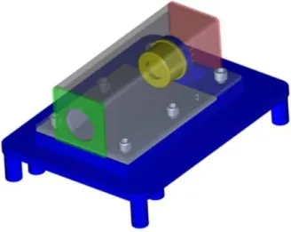
Figure 1.Schematic of an X-ray detector assembly (Zajczyk et al. 2018). The SDD is shown in gold. The copper-tungsten passive shield is shown in gray with the top part semi-transparent, the for-ward end cap in green with the sky aperture, and the rear end cap in red. The detector is mounted on an aluminum baseplate shown in blue with the front-end electronics (not shown) mounted on the bottom of the plate.
a thermoelectric cooler package viewing the sky through a Si3N4 window covered with a thin layer of aluminum. The SDD is cooled to -30 C during operation, but the window re-mains at ambient temperature which should help reduce the buildup of contaminants. The SDD provides no imaging ca-pability.
Each detector is mounted in a compartment inside the in-strument chassis made of aluminum. To minimize back-ground from charged particle interactions and the diffuse X-ray background, each SDD is surrounded by a shield made of 1.2 mm thick copper-tungsten metal matrix composite elec-troplated with a 2.5 µm layer of nickel and an outer 1.3 µm layer of gold, see Fig.1. The shield has a circular aperture through which the SDD views the sky, see Fig.2. There is a 0.78 mm thick aluminum washer at the front of each de-tector compartment with a circular aperture that defines the field of view (FoV). The full-response radius was measured in ground testing to be5.02◦ and the zero-response radius to be7.03◦with a linear decrease between. The response-weighted effective field of view is 0.0350 steradians.
Each X-ray creates a charge pulse. Pulses triggering a lower level discriminator are digitized and the pulse height and time of arrival, with a resolution of 0.05 s, are recorded by a data-processing unit (DPU) which is a field-programmable gate array programmed with a microprocessor core. We refer to the detector units using numbers encoded into their DPUs which are 14, 54, and 38 as viewed from left to right in Fig.2.
The X-ray energy to pulse height conversion was measured during ground calibration with the detectors illuminated by an X-ray beam with fluorescence emission at the F Kα line (676.8 eV) from a Teflon target along with lines from Al, Si,
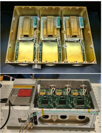
Figure 2. Top - The three flight detectors mounted in the instru-ment chassis. The passive shields are visible towards the back; the detectors are inside. The brass housings towards the front are high-voltage power supplies. The X-ray apertures are at the front. Bot-tom - Science instrument mounted in the flight bus chassis. Printed circuit boards for analog electronics and the DPUs are on the top of instrument chassis with the alignment washers and a cover over a flat mirror used for optical alignment at the front. The instrument cover and solar array are not attached.
Cr, and Fe, and by a55
Fe radioactive source (Zajczyk et al. 2018). Measurements were made at instrument temperatures ranging from−25 C to +40 C. The pulse height to X-ray en-ergy conversion is linear with a non-zero offset. The offset is a linear function of temperature while the slope is a quadratic function of temperature. The energy scale shifts are up to ∼15 eV across the range from −25 C to +40 C. Details of the ground calibration are presented inZajczyk et al.(2019). The energy resolution averaging over all temperatures was measured to be88.3 ± 3.5, 84.3 ± 2.8, and 82.0 ± 1.4 eV (FHWM) at the F Kα line and138.5 ± 2.1, 136.5 ± 0.8, and 137.3 ± 1.9 eV (FWHM) at the Mn Kα line (the intensity-weighted average of the Kα1and Kα2lines is 5895.0 eV) for DPUs 14, 54, and 38, respectively.
Detector response matrices were prepared using soft-ware that models the response of silicon detectors
(Scholze & Procop 2009). The software was modified for
the SDDs used for NASA’s Neutron star Interior Compo-sition Explorer (NICER) instrument (Gendreau et al. 2016)
0.5
1
2
5
Energy (keV)
0.01
0.02
0.05
0.1
0.2
Effe
cti
ve
ar
ea
(c
m
2)
Figure 3.Effective area versus energy of a single HaloSat SDD.
and kindly provided to us by Dr. Jack Steiner of MIT. The NICER SDDs are identical to those on HaloSat except for use of a thinner window. We adjusted the relevant detector parameters using the ground calibration data and informa-tion on the windows supplied by Amptek, Inc., and HS-Foils, Oy. The effective area of a single HaloSat SDD is shown in Fig.3. The response files are compatible with the Xspec spectral fitting software (Arnaud 1996) which is commonly used in X-ray astronomy to enable use of HaloSat data by the astronomical community.
4. SPACECRAFT AND OPERATIONS
To minimize development costs and enhance the proba-bility of mission success by the use of flight-proven com-ponents, we chose to use a commercial CubeSat ‘bus’ pro-vided by Blue Canyon Technologies, Inc., (BCT) to provide attitude control, command and data handling, and a power system. Power is provided by a deployable solar array that charges the on-board batteries during the day side of the spacecraft orbit. The spacecraft can be slewed at a 2◦ per second rate and has a pointing accuracy of ±0.002◦ (1σ)
(Hegel 2016). An on-board CADET radio is used to
down-link telemetry to and receive commands from a radio ground station at NASA’s Wallops Flight Facility. A GlobalStar ra-dio provides occasional housekeeping information.
Blue Canyon Technologies performs mission operations based on observation plans generated at the University of Iowa (UI). All the instrument telemetry (which includes X-ray event data, instrument housekeeping data, and spacecraft attitude and orbit information) is captured in a database and processed into a set of FITS (Flexible Image Transport Sys-tem) format files including spectra and event lists for each target. The FITS files will be archived at the High Energy Astrophysics Science Archive Research Center (HEASARC) and made publicly available within 5 months after mission completion.
0 2 4 6 8 Offset from center (deg)
0.0 0.2 0.4 0.6 0.8 1.0 1.2 1.4 Co un t r ate (c /s)
Figure 4.X-ray count rate versus pointing offset from the Crab for DPU 54.
Table 1.Pointing offsets. DPU X(deg) Y (deg) 14 -0.11 0.18 54 -0.01 0.15 38 -0.05 0.10
5. ON-ORBIT PERFORMANCE
The first observations with HaloSat were done to measure the instrument pointing and field of view and to verify the spectral response and effective area.
5.1. Pointing and Field of View
The Crab is a pulsar wind nebula powered by a young pul-sar with a spin period of about 33 ms. The Crab has been used as a calibration target since the early days of X-ray astronomy
(Toor & Seward 1974). We used the Crab to measure the
alignment between the boresights of the X-ray instruments and the coordinate system defined by the star trackers on the spacecraft bus.
We performed a series of slew maneuvers in which the sci-ence instrument was pointed towards the Crab and then the pointing was gradually offset while the spacecraft roll angle was held fixed. Eight different maneuvers were performed corresponding to eight different roll angles at equal inter-vals in the spacecraft frame. The X-ray count rate versus offset data were fit to a model matching the FoV measured on the ground with the center being a fit parameter. Good fits were obtained, see Fig.4, verifying the ground FoV measure-ments. We found an offset of about1.0◦in the spacecraft Y direction from the nominal pre-flight instrument boresight. This correction was applied to the pointing of observations obtained after 1 December 2018.
After the correction, another pointing test was performed and the best fit FoV center was found to be consistent with the
6
7
8
9
10
No
rm
ali
ze
d c
o
nts/s/ke
V
14
54
38
1.0
1.5
2.0
2.5
Energy (keV)
−2.5
0.0
2.5
Δ
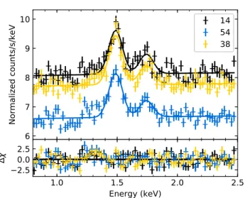
χFigure 5. X-ray spectra of the dark Earth. Data from all three detectors are shown as indicated by the DPU numbers in the legend. Emission lines are visible from neutral Al at 1.49 keV and neutral Si at 1.74 keV.
expected position within±0.11◦ in the spacecraft X direc-tion and±0.18◦in the spacecraft Y direction for all DPUs, see Table1. The count rate for DPU 54 versus radial offset from the best fit center for the best fit model is shown in Fig.4
and the pointing offsets for each detector are presented in Ta-ble1. The uncertainties on the offsets are±0.05◦(1σ). We conclude that the pointing of the X-ray boresight of HaloSat is accurate to within ±0.23◦, which is a small fraction of the FoV. The X-ray pointing uncertainty is dominated by the accuracy to which we are able to measure the relative align-ment between the X-ray detectors and the spacecraft refer-ence frame. The median offset between the commanded tar-get position during observations and the spacecraft pointing measured by the attitude control system is 0.0007◦.
5.2. Spectral Response
To check the on-orbit X-ray energy scale calibration, we examined spectra obtained while observing the dark side of the Earth and while observing the supernova remnant (SNR) Cassiopeia A.
The dark Earth observations show instrumental lines from aluminum and silicon likely due to fluorescence by ener-getic particles. Data were processed using the temperature-dependent ground energy calibration and filtered to maxi-mize the significance of these lines. The resulting spectra were fit with a model consisting of two Gaussians and a pow-erlaw, see Fig.5. With the line centroid energies fixed to the average of the laboratory values of the Kα1, Kα2, and Kβ lines weighted by their relative strengths (1.4875 keV for Al and 1.7425 keV for Si), we obtained a good fit with χ2
/DoF = 337.7/239. Allowing the line centroid energies to vary did not produce a significant improvement in the fit with an F-test probability of 0.35. The line centroid error ranges include the weighted laboratory values and the best fit centroids for the Al line are all within 3 eV of the laboratory value.
1
2
3
0.02
0.05
0.1
0.2
No
rm
ali
ze
d c
ou
nts/s/ke
V
14
54
38
1
2
3
Energy (keV)
−4
−2
0
2
χFigure 6. X-ray spectra of the Cas A field in the 1-3.5 keV band. Data from all three detectors are shown as indicated by the legend. Prominent emission lines are visible from Si XIII at 1.86 keV and S XV at 2.45 keV. Table2shows the lines used in fitting the spectra.
Table 2.X-ray lines from Cas A. Line Energy (keV) EW (keV) Mg Heα 1.3375 0.04 Si Heα 1.8558 0.40 Si Lyα 2.0053 0.13 Si Heβ 2.1830 0.13 Si Lyβ 2.3770 0.06 S Heα 2.4510 0.17 S Lyα 2.6220 0.09 S Heβ 2.9218 0.09 Ar Heα 3.1400 0.13
Cas A has strong emission lines from heavy elements in its X-ray spectrum. X-ray emission lines from Mg, Si, S, and Ar were first detected with the solid-state spectrometer on Einstein (Becker et al. 1979) and first mapped with ASCA
(Holt et al. 1994). Cas A has been used to calibrate the
en-ergy scale of previous X-ray instruments (Jahoda et al. 2006). The HaloSat field centered on Cas A includes another SNR, CTB 109, and several point sources, but the emission is dominated by Cas A. We extracted spectra of the Cas A for all three DPUs, see Fig.6, and fit them in the 1.0-3.5 keV range with a model consisting of a powerlaw and nine Gaussians for the astrophysical emission and a powerlaw with photon index fixed to 0.65 for the instrumental background that was not modified by the response matrix. The parameters of the astrophysical model were set equal for the different detec-tors while the normalization of the instrumental background was allowed to vary between detectors. Line energies were extracted from the AtomDB database of atomic transitions
0.05
0.1
0.2
0.5
No
rm
ali
ze
d c
ou
nts/s/ke
V
14
54
38
0.5
1
2
5
Energy (keV)
−4
−20
24
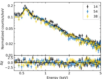
χFigure 7. X-ray spectra of the Crab in the 0.5-7 keV band. Data from all three detectors are shown as indicated by the legend.
Table 3.Crab flux from various instruments.
Instrument Norm Γ NH Flux
Historical 9.7±1.0 2.100±0.030 3.54 11.0 RXTE/PCA 11.02±0.04 2.120±0.002 3.54 12.4 NuSTAR 9.71±0.16 2.106±0.006 3.54 11.0 HaloSat 10.20±0.17 2.12±0.03 3.54±0.13 11.5
NOTE—Normalization is in units ofphotons keV−1cm−2s−1at
1 keV and NH is in units of 1021cm−2. Flux is in the
0.5-2 keV band in units of (10−9erg cm−2s−1). References are:
Toor & Seward(1974) for the historical instruments, Kirsch et al. (2005) for the PCA, andMadsen et al.(2017) for NuSTAR.
and centroids for blends were calculated from their relative intensities and are given in Table2.
The continuum X-ray spectrum of Cas A is typically de-scribed as the sum of two thermal plasma components and a powerlaw, but a single powerlaw produces an adequate fit over the limited energy band used in the fit with χ2
/DoF = 438.31/358. The best fit equivalent widths (EW) for the de-tected lines are presented in Table 2. The line widths are consistent with the energy resolution measured during the ground calibration. Allowing the slope or the intercept of the channel to energy conversion to vary did not significantly improve the fit with F-test probabilities of 0.20 and 0.16, re-spectively. The best fit response slopes differ by less than 0.2% from the ground calibration while the best fit intercepts differ by less than 5 eV.
5.3. Effective Area
We used the Crab to check the effective area of HaloSat. The Crab is often used as a ‘standard candle’ in X-ray astron-omy (Toor & Seward 1974;Jahoda et al. 2006;Madsen et al. 2015). However, it does exhibit variability of up to 7% in the
10-100 keV band on long time scales (Wilson-Hodge et al.
2011).
We extracted Crab spectra for each detector, see Fig.7, and applied the temperature-dependent energy calibration and response matrices discussed previously. We mod-eled the Crab spectrum as an absorbed powerlaw with the TBabs model in Xspec to describe the interstellar absorp-tion (Wilms, Allen, & McCray 2000). The same absorp-tion column density, NH, and powerlaw photon index, Γ, were used for all detectors, but the normalization was al-lowed to vary between the detectors. We included a pow-erlaw with photon index and normalization fixed to the val-ues found by Cappelluti et al. (2017) to model the cosmic X-ray background (CXB) subject to absorption with the TBabs model with the column density fixed to the average Galactic absorption within a 5◦ radius of the line of sight
(HI4PI Collaboration et al. 2016). We added a powerlaw not
modified by the response matrix to model the instrumental background. The instrumental background photon index was fixed to 0.65 and the normalization was allowed to vary be-tween the detectors. We fitted the spectra in the 0.4-7 keV band.
We obtained a good fit with χ2
/DoF = 1227.5/979 for NH = (3.54 ± 0.13) × 1021
cm−2 andΓ = 2.12 ± 0.03 (90% confidence). The photon index is consistent with those measured for the Crab with XMM-Newton, the Proportional Counter Array (PCA) on the Rossi X-ray Timing Explorer
(Kirsch et al. 2005), and NuSTAR (Madsen et al. 2017), see
Table3. We note that the photon index depends on the energy band used for the fitting. If we use a softer band, we find a harder photon index, consistent with the values reported for instruments sensitive in softer bands such as the Low En-ergy Concentrator Spectrometer on BeppoSAX and the Posi-tion Sensitive ProporPosi-tional Counter on ROSAT (Kirsch et al. 2005). This suggests that a single power law does not provide an adequate representation of the spectrum of the Crab pulsar plus nebula at low energies, consistent with the observations that the pulsed flux is harder than the nebular emission.
The science of HaloSat is focused on emission in the 0.5-2 keV band. The Crab flux in that band depends on all of the model parameters, so we prefer to directly compare ob-served fluxes rather than only the powerlaw normalization. The HaloSat fluxes from the Crab in the 0.5-2 keV band in units of 10−9erg cm−2s−1 are 11.54 ± 0.20 for DPU 14, 11.74 ± 0.21 for DPU 54, and 11.27 ± 0.20 for DPU 38 (uncertainties are 90% confidence). The fluxes are consis-tent within the statistical error. The CXB contributes 4% of the total counts in the 0.5-2 keV band while the instrumental background contributes 8% to 10% depending on the detec-tor. Thus, uncertainty in modeling the instrumental back-ground may contribute up to a few per cent uncertainty in measuring the Crab flux.
We compare the HaloSat Crab flux in the 0.5-2 keV band with the flux calculated from the spectral parameters,Γ and normalization, measured with other instruments in Table3.
Madsen et al.(2017) recently measured the absolute flux of
the Crab using a NuSTAR observation in which the
detec-tors were illuminated directly without the X-rays passing through the optics. This greatly simplifies the instrument re-sponse. They found that the true Crab flux in the 3-7 keV band is∼12% higher than their previous choice for the Crab normalization based on results from contemporary missions with X-ray optics. This motivates our choice of collimated instruments for comparison. Because those measurements do not extend to the soft band needed to accurately measure the absorption, we use the absorption measured by HaloSat. We find that the Crab flux as measured by HaloSat agrees within 8% with that inferred from the PCA spectral parame-ters and within 5% with that inferred from the NuSTAR pa-rameters and the average of historical spectral papa-rameters in
Toor & Seward(1974). Due to the uncertainty in
extrapolat-ing these measurements to the soft X-ray band and the sim-plicity of the response of HaloSat, we choose not to make any adjustments to the effective area of HaloSat.
Most of the previously published results on Milky Way halo emission use XMM-Newton which has two imaging in-struments, the EPIC-MOS and the EPIC-pn. Unfortunately, the MOS suffers from pileup during observations of the Crab and the only Crab normalizations reported are for the EPIC-pn. Using the parameters of the Crab spectrum measured
byKirsch et al.(2005) for the EPIC-pn using Wilms
abun-dances and Verner cross-sections, we find an absorbed flux of(9.185 ± 0.042) × 10−9erg cm−2s−1 in the 0.5-2 keV band. Cross calibrating the MOS and PN, Mateos et al.
(2009) found that the MOS registers higher flux than the pn with the ratio being energy dependent. Averaging their val-ues for the ratio of pn versus MOS1 and MOS2 in the 0.5-1 and 1-2 keV energy bands, we find a correction factor for the 0.5-2 keV band of 8.4%. Comparing their NuSTAR ab-solute Crab flux measurement with the EPIC-MOS in the 3-7 keV band,Madsen et al. (2017) found that the MOS flux was 11.6% lower. Combining these two factors, we con-clude that the Crab pn flux should be corrected by a factor of 1.21, bringing the flux to11.1 × 10−9erg cm−2s−1. This is about 4% lower than the HaloSat Crab flux. This is rea-sonable agreement given the uncertainties.
5.4. Background
HaloSat was deployed from the ISS and has an orbital in-clination of 51.6◦ which brings the spacecraft into regions of high background at the high and low latitude regions of the orbit as well as in the South Atlantic Anamoly (SAA), see Fig.8. The SAA covers a well defined region and has a consistently high particle background. Instrument event pro-cessing is automatically turned off upon entrance to the SAA and resumed upon exit. The background at all latitudes is time variable. Data are collected in these regions and filters are applied in the data analysis to select times when the in-strumental background is low. Optimization of the filtering algorithms and background modeling is currently underway. We note that the orbital inclination of the ISS is not opti-mal for HaloSat because of the high instrumental background experienced mostly at high latitudes. Development of the ca-pability for routine small satellite launches at lower
inclina-−100 0 100 Longitude (deg) −50 −25 0 25 50 La ti tu de ( de g) 0.00 0.25 0.50 0.75 1.00 Count Rate (cts/s)
Figure 8.Median count rate before background filtering versus or-bital position for DPU 38 in the energy band 0.4-3 keV. The SAA is prominent and high background regions at high latitudes are visible.
tions of 30◦or less would benefit future high energy astro-physics small satellite missions by providing lower instru-mental background and increased observational efficiency.
6. INITIAL HALO OBSERVATIONS
To make a useful contribution to the study of the hot halo of the Milky Way, HaloSat must achieve its design sensi-tivity for oxygen line emission and it must survey a large fraction of the high Galactic latitude sky. Figure 9 shows a spectrum obtained for a high Galactic latitude field at (l = 165.59◦, b = 61.92◦). We also analyzed data for a second field at(229.25◦
,67.50◦) The temperature-dependent energy calibration described above was applied.
FollowingHenley & Shelton(2012), we fit the data with a model consisting of Gaussians with centroids fixed at 568.4 eV and 653.7 eV for the O VII and O VIII line emission and an absorbed thermal plasma model (APEC) for emission from the halo and an unabsorbed APEC model for emission from the local bubble (LB). We fixed the tem-perature and emission measure for the local bubble APEC model using the results fromLiu et al.(2017). We removed the oxygen line emission from the APEC models following the procedure ofLei et al.(2009), but only removing lines in the energy range from 0.484 to 0.744 eV which covers that modeled with the two Gaussians. We included a pow-erlaw with photon index fixed to 1.45 to model the CXB
(Cappelluti et al. 2017). The halo APEC component and the
CXB powerlaw component were subject to absorption with the TBabs model with the column density fixed to the aver-age Galactic absorption within a5◦radius of the line of sight
(HI4PI Collaboration et al. 2016). We added a powerlaw not
modified by the response matrix to model the instrumental background. The instrumental background photon index was fixed to 0.65 and the normalization was allowed to vary be-tween the detectors. We used the C-statistic to perform fitting
0.01
0.02
0.05
0.1
0.2
No
rm
ali
ze
d c
ou
nts/s/ke
V
14
54
38
0.5
1
2
5
Energy (keV)
−2.5
0.0
2.5
χFigure 9.X-ray spectra of a halo field. Data from all three detectors are shown as indicated by the legend.
Table 4.Halo spectrum model parameters.
Parameter (229.25, 67.50) (165.59, 61.92) Exposure (ks) 42.6, 42.2, 41.9 44.4, 44.0, 42.7 OVIIflux (LU) 5.14±0.39 4.33±0.35 OVIIIflux (LU) 0.94±0.20 0.90±0.18 NH(1020cm−2) 1.41 1.13 Halo kT (keV) 0.178±0.007 0.189±0.010 Halo EM (10−3 cm−6 pc) 25.8±4.3 19.8±3.8 LB kT (keV) 0.097 0.097 LB EM 4.14 4.70 CXBΓ 1.45 1.45 CXB norm 10.3±0.7 9.3±0.6 χ2/DoF 776.1/679 799.64/679
NOTE—Uncertainties are 1σ confidence. Quantities without uncer-tainties were held fixed. The exposures are after background and data quality screening for DPU 14, 54, and 38. The CXB normal-ization is at 1 keV with units ofkeV cm−2s−1sr−1keV−1.
and the χ2
-statistic to evaluate the quality of fit. Fitting over the 0.4-5 keV band.
The fit parameters are shown in Table4. The statistical ac-curacy on the O VIIflux meets our observational goal. The O VII flux for the field at(l = 165.59◦, b = 61.92◦) is lower than the fluxes measured byHenley & Shelton(2012) using XMM-Newton for lines of sight within the HaloSat field which range from 5.34±0.44 LU to to 8.47±0.24 LU. The flux for the field at (l = 230.1◦, b = 66.2◦) is slightly higher than the fluxes of 3.54±0.36 LU and 3.16±0.28 LU
fromHenley & Shelton(2012) in the same field. The CXB
normalizations are in reasonable agreement with that of
0 ° 1 2 3 4 5 6 7 8 9 1 0 1 1 1 2 1 3 1 4 1 5 1 6 1 7 1 8 1 9 2 0 2 1 2 2 2 3 2 4 2 5 2 6 2 7 2 8 2 9 3 0 3 1 3 2 3 3 3 4 3 5 3 6 3 7 3 8 3 9 4 0 4 1 4 2 4 3 4 4 4 5 4 6 4 7 4 8 4 9 5 0 5 1 5 2 5 3 5 4 5 5 5 6 5 7 5 8 5 9 6 0 6 1 6 2 6 3 6 4 6 5 6 6 6 7 6 8 6 9 7 0 7 1 7 2 7 3 7 4 7 5 7 6 7 7 7 8 7 9 8 0 8 1 8 2 8 3 8 4 8 5 8 6 8 7 8 8 8 9 9 0 9 1 9 2 9 3 9 4 9 5 9 6 9 7 9 8 9 9 1 0 0 1 0 1 1 0 2 1 0 3 1 0 4 1 0 5 1 0 6 1 0 7 1 0 8 1 0 9 1 1 0 1 1 1 1 1 2 1 1 3 1 1 4 1 1 5 1 1 6 1 1 7 1 1 8 1 1 9 1 2 0 1 2 1 1 2 2 1 2 3 1 2 4 1 2 5 1 2 6 1 2 7 1 2 8 1 2 9 1 3 0 1 3 1 1 3 2 1 3 3 1 3 4 1 3 5 1 3 6 1 3 7 1 3 8 1 3 9 1 4 0 1 4 1 1 4 2 1 4 3 1 4 4 1 4 5 1 4 6 1 4 7 1 4 8 1 4 9 1 5 0 1 5 1 1 5 2 1 5 3 1 5 4 1 5 5 1 5 6 1 5 7 1 5 8 1 5 9 1 6 0 1 6 1 1 6 2 1 6 3 1 6 4 1 6 5 1 6 6 1 6 7 1 6 8 1 6 9 1 7 0 1 7 1 1 7 2 1 7 3 1 7 4 1 7 5 1 7 6 1 7 7 1 7 8 1 7 9 1 8 0 1 8 1 1 8 2 1 8 3 1 8 4 1 8 5 1 8 6 1 8 7 1 8 8 1 8 9 1 9 0 1 9 1 1 9 2 1 9 3 1 9 4 1 9 5 1 9 6 1 9 7 1 9 8 1 9 9 2 0 0 2 0 1 2 0 2 2 0 3 2 0 4 2 0 5 2 0 6 2 0 7 2 0 8 2 0 9 2 1 0 2 1 1 2 1 2 2 1 3 2 1 4 2 1 5 2 1 6 2 1 7 2 1 8 2 1 9 2 2 0 2 2 1 2 2 2 2 2 3 2 2 4 2 2 5 2 2 6 2 2 7 2 2 8 2 2 9 2 3 0 2 3 1 2 3 2 2 3 3 2 3 4 2 3 5 2 3 6 2 3 7 2 3 8 2 3 9 2 4 0 2 4 1 2 4 2 2 4 3 2 4 4 2 4 5 2 4 6 2 4 7 2 4 8 2 4 9 2 5 0 2 5 1 2 5 2 2 5 3 2 5 4 2 5 5 2 5 6 2 5 7 2 5 8 2 5 9 2 6 0 2 6 1 2 6 2 2 6 3 2 6 4 2 6 5 2 6 6 2 6 7 2 6 8 2 6 9 2 7 0 2 7 1 2 7 2 2 7 3 2 7 4 2 7 5 2 7 6 2 7 7 2 7 8 2 7 9 2 8 0 2 8 1 2 8 2 2 8 3 2 8 4 2 8 5 2 8 6 2 8 7 2 8 8 2 8 9 2 9 0 2 9 1 2 9 2 2 9 3 2 9 4 2 9 5 2 9 6 2 9 7 2 9 8 2 9 9 3 0 0 3 0 1 3 0 2 3 0 3 3 0 4 3 0 5 3 0 6 3 0 7 3 0 8 3 0 9 3 1 0 3 1 1 3 1 2 3 1 3 3 1 4 3 1 5 3 1 6 3 1 7 3 1 8 3 1 9 3 2 0 3 2 1 3 2 2 3 2 3 3 2 4 3 2 5 3 2 6 3 2 7 3 2 8 3 2 9 3 3 0 3 3 1 3 3 2 3 3 3
Figure 10.HaloSat targets in Galactic coordinates. The Galactic center is at the center of the image, longitude increases to the left, and latitude increases toward the top. The blue contours show the 10◦diameter full-response field of view for each target and the yellow contours show the
14◦diameter zero response. The black Xs show bright X-ray sources.
Table 5.HaloSat targets
ID Name Type RA DEC l b
1 Cygnus Loop C 312.75 30.67 73.98 -8.56 2 Sco X-1 C 244.98 -15.64 359.09 23.78 3 Crab C 83.63 22.01 184.56 -5.78 . . . 8 LMC S 78.83 -67.78 278.32 -34.00 9 Pup A offset S 118.07 -39.33 254.27 -6.22 10 Tycho SNR S 5.79 64.66 119.91 1.95 . . . 66 HSWCX1 X 73.27 17.51 182.73 -16.37 67 HSWCX2 X 101.92 -61.29 271.21 -24.01 68 MSWCX1 X 15.46 18.24 126.40 -44.56 . . . 80 HALO J1807+699 H 271.83 69.98 100.31 29.12 81 HALO J0011+119 H 2.86 11.94 107.69 -49.75 82 HALO J0021-440 H 5.45 -44.07 320.42 -72.04 83 HALO J0021-255 H 5.44 -25.57 44.48 -83.17 . . .
NOTE—Type: C = Calibration, S = Secondary science, X = Solar wind charge exchange, H = Halo. RA and DEC are J2000 coordinates. l and bare Galactic coordinates. This table is published in its entirety in the machine-readable format. A portion is shown here for guidance regarding its form and content.
In order to measure the properties of the halo, we must conduct similar observations over a large fraction of the sky. Our goal is to survey the entire sky, although the fields with |b| > 30◦will be most useful in constraining the properties
of the halo. The size of the FoV determines the number of targets needed to cover the sky. We selected 333 targets to tile the sky including targets selected for instrument calibration, SWCX studies, and secondary science on bright, extended soft X-ray sources. The positions of the halo targets were chosen to minimize overlap and avoid bright X-ray sources in the ROSAT, Uhuru, and MAXI catalogs, particularly those with low-energy line features. The targets are presented in Table5and shown in Galactic coordinates in Fig10.
7. CONCLUSIONS
The initial results presented here demonstrate that HaloSat should help advance our understanding of the hot halo of the Milky Way and provide a unique data set for the study of so-lar wind charge exchange emission. Thus, CubeSats can be effective vehicles for astrophysics research even within their limited mass, power, and volume constraints and be con-structed and operated at modest cost by exploiting the com-mercialization of small satellite technologies. The success of HaloSat should encourage construction of more CubeSats for astrophysics.
ACKNOWLEDGMENTS
We acknowledge support from NASA grant NNX15AU57G. We thank Steve Schneider for leading the bus work, Tracy Behrens for her tireless work in assembling the HaloSat electronics, Luis Santos for system engineering, Keith White for mechanical design and drawing, Chris Esser for spacecraft mechanical design, Tom Golden and Doug Laczkowksi for mission operations, Rich Dvorsky for me-chanical and polymerics advice, and Jeff Dolan for advice about connectors and electronics.
We are grateful to Brian Busch, Larry Detweiler, and Matt Miller for machining parts, Kayla Racinowski for help with polymerics, Jim Phillips for help with inductor cores, Jesse Haworth for HVPS testing and designing the logo, Riley Wearmouth for early mechanical designs, Mike Matthews for work on the concept of operations and communications, Brenda Dingwall for program management, Calvin Whitaker and Tyler Roth for system administration, Tim Cameron for building the HVPS, and John Hudeck for seeing us through instrument vibration testing and for mentoring Keith White.
Our reviewers, Dave Sheppard, Scott Porter, Kevin Black, and Jasper Halekas, provided an invaluable service.
Kris-ten Hanslik, Charles Dumont, Karl Hansen, Bruce Patterson, Natali Vannoy, Jake Beckner, David Hall, Jesse Ellison, and Matt Pallas did a great job seeing us through integration and testing, as did Scott Inlow on thermal modeling, Matt Baum-gart and Bryan Rogler on GNC engineering, Nick Monahan, Austin Bullard, and Jeff Adams on mission operations, Re-becca Walter on RF engineering, and Steve Bundick and Matt Schneider on communications testing.
We couldn’t talk to HaloSat without the WFF UHF Ground Station Team and their continuing support. We thank De-von Sanders, Ned Riedel, Allen Crane, Larry Madison, and Kyle McLean for their work on alignment, Dan Evans and Mike Garcia for help from above, and Tristan Prejean, Conor Brown, and many others at Nanoracks for getting HaloSat into orbit. We probably wouldn’t have been selected without the work of Ben Cervantes, Will Mast, Scott Schaire, Ryoichi Hasebe, Brad Hood, Sally Smith, and Brooks Flaherty on the Mission Planning Laboratory run for the proposal.
Facility:
HaloSatSoftware:
XSPEC (Arnaud 1996), astropy(Astropy Collaboration et al. 2013)
REFERENCES
Aschenbach, B., Egger, R., & Tr¨umper, J., Discovery of Explosion Fragments Outside the Vela Supernova Remnant Shock-Wave Boundary, Nature, 373, 587, 1995.
Arnaud, K.A. 1996, ASP Conf., 101, 17
Astropy Collaboration, Robitaille, T. P., Tollerud, E. J., et al. 2013, A&A, 558, A33
Becker, R.H., Holt, S.S., Smith, B.W. et al. 1979, ApJ, 234, L73 Boylan-Kolchin, M., Bullock, J. S., Sohn, S. T. et al. 2013, ApJ,
768, 140
Cappelluti, N., Li, Y., Ricarte, A., et al. 2017, ApJ, 837, 19 Cen, R. and Ostriker, J.P. 1999, ApJ, 514, 1
Crusan, J. & Galica, C. 2019, Acta Astronautica, 157, 51 Dame, T.M. 1993, AIP Conf. Ser., 278, 267
Galeazzi, M., Chiao, M., Collier, M.R. et al. 2014, Nature, 512, 171 Gendreau, K.C., Arzoumanian, Z., Adkins, P. W. et al. 2016, Proc.
SPIE, 9905, 99051H
Grcevich, J. & Putnam, M. E. 2009, ApJ, 696, 385
Gupta, A., Mathur, S., Krongold, Y., Nicastro, F., and Galeazzi, M., ApJ, 756, L8
Hegel, D. 2016, in 30th Annual AIAA/USU Conference on Small Satellites, SSC16-X-7,
https://digitalcommons.usu.edu/smallsat/2016/TS10AdvTech2/5/ Henley, D.B., Shelton, R.L., Kwak, K., Joung, M. R., Mac Low,
M.-M. 2010, ApJ, 723, 935
Henley, D.B. & Shelton, R.L. 2012, ApJS, 202, 14
Hevner, R., Holemans, W., Puig-Suari, J., Twiggs, R. 2011, Proceedings of the AIAA/USU Conference on Small Satellites, From 0 to 7.5 km/s, SSC11-II-3,
https://digitalcommons.usu.edu/smallsat/2011/all2011/15/ HI4PI Collaboration, Ben Bekhti, N., Fl¨oer, L., et al. 2016, A&A,
594, A116
Holt, S.S., Gotthelf, E.V., Tsunemi, H., Negoro, H. 1994, PASJ, 46, L151
Jahoda, K., Markwardt, C.B., Radeva, Y. et al. 2006, ApJS, 163, 401
Kaaret, P., Zajczyk, A., LaRocca, D. et al. 2019, Proceedings of the AIAA/USU Conference on Small Satellites, Year in Review I, SSC19-III-05,
https://digitalcommons.usu.edu/smallsat/2019/all2019/277/ Kirsch, M.G., Briel, U.G., Burrows, D. et al. 2005, Proc. SPIE,
5898, 22
Koutroumpa, D., Collier, M.R., Kuntz, K.D. et al. 2009, ApJ, 697, 1214
Kuntz, K.D. 2019, A&AR, 27, 1
Lei, S., Shelton, R. L., Henley, D. B. 2009, ApJ, 699, 1891 Liu, W., Chiao, M., Collier, M. R. et al. 2017, ApJ, 834, 33 Madsen, K.K., Harrison, F.A., Markwardt, C.B. et al. 2015, ApJS,
220, 8
Madsen, K.K., Forster, K., Grefenstette, B.W., Harrion, F.A., Stern, D. 2017, ApJ, 841, 56
Mateos, S., Saxton, R.D., read, A.M., Sumbay, S. 2009, A&A, 496, 879
McMillan, P.J. 2011, MNRAS, 414, 2446-2457 Miller, M. J. & Bregman, J. N. 2015, ApJ, 800, 14
Moretti, A., Pagani, C., Cusumano, G. et al. 2009, A&A, 493, 501 Nicastro, F., Zezas, A., Drake, J. et al. 2002, ApJ, 573, 157 Planck Collaboration, 2014, A&A, 571, A16
Revnivtsev, M., Gilfanov, M., Jahoda, K., Sunyaev, R. 2005, A&A, 444, 381
Scholze, F. & Procop, M. 2009, X-Ray Spectrometry, 38, 312321 Shull, J.M., Smith, B.D., & Danforth, C.W. 2012, ApJ, 759, 23 Slavin, J., Wargelin, B.J., & Koutroumpa, D. 2013, ApJ, 779, 13 Smith, R.K., Bautz, M. W., Edgar et al. 2007, PASJ, 59, 141 Snowden, S.L., Egger, R., Freyberg, M. J. et al. 1997, ApJ, 485,
125
Spitzer, L. 1956, ApJ, 124, 20
Toor, A. & Seward, F. D. 1974, AJ, 79, 995
Weisskopf, M.C., Guainazzi, M., Jahoda, K. et al. 2010, ApJ, 713, 912
Wilms, J., Allen, A., & McCray, R. 2000, ApJ, 542, 914 Wilson-Hodge, C.A., Cherry, M.L., Case, G.L. et al. 2011, ApJ,
727, L40
Yoshino, T., Mitsuda, K., Yamasaki, N. Y. et al. 2009, PASJ, 61, 805
Zajczyk, A., Kaaret, P., Kirchner, D.L. et al. 2018, Proceedings of the AIAA/USU Conference on Small Satellites, Upcoming Missions, SSC18-WKIX-01,
https://digitalcommons.usu.edu/smallsat/2018/all2018/471/ Zajczyk, A., Kaaret, P. et al. 2019, in preparation.
Zhezher, Ya. V., Nugaev, E. Ya., & Rubtsov, G. I. 2017, Astron. L., 42, 173-181