HAL Id: hal-00318308
https://hal.archives-ouvertes.fr/hal-00318308
Submitted on 8 May 2007
HAL is a multi-disciplinary open access
archive for the deposit and dissemination of
sci-entific research documents, whether they are
pub-lished or not. The documents may come from
teaching and research institutions in France or
abroad, or from public or private research centers.
L’archive ouverte pluridisciplinaire HAL, est
destinée au dépôt et à la diffusion de documents
scientifiques de niveau recherche, publiés ou non,
émanant des établissements d’enseignement et de
recherche français ou étrangers, des laboratoires
publics ou privés.
the HF Doppler technique
D. Buresova, V. Krasnov, Ya. Drobzheva, J. Lastovicka, J. Chum, F. Hruska
To cite this version:
D. Buresova, V. Krasnov, Ya. Drobzheva, J. Lastovicka, J. Chum, et al.. Assessing the quality of
ionogram interpretation using the HF Doppler technique. Annales Geophysicae, European Geosciences
Union, 2007, 25 (4), pp.895-904. �hal-00318308�
Ann. Geophys., 25, 895–904, 2007 www.ann-geophys.net/25/895/2007/ © European Geosciences Union 2007
Annales
Geophysicae
Assessing the quality of ionogram interpretation using the HF
Doppler technique
D. Buresova1, V. Krasnov1,2, Ya. Drobzheva1,2, J. Lastovicka1, J. Chum1, and F. Hruska1 1Institute of Atmospheric Physics, 14131 Prague, Czech Republic
2Institute of the Ionosphere, Almaty, Republic of Kazakhstan
Received: 22 December 2005 – Revised: 13 February 2007 – Accepted: 30 March 2007 – Published: 8 May 2007
Abstract. The first joint common volume measurements by the Digisonde Portable Sounder (DPS-4) and a new Doppler type system has been run at the Pruhonice ionospheric obser-vatory (49.99◦N, 14.54◦E) since January 2004. The mea-surement of the Doppler shift is carried out continuously on a frequency of 3.6 MHz, thus the radio wave is reflected predominantly from the ionospheric F layer. To compare digisonde measurements with the Doppler data, a phase path was calculated from both Doppler and digisonde records. Under stormy conditions and in the case where a sporadic E layer was present, a significant disagreement between both measurements has been found. The discrepancies could be related to the uncertainties of the observational inputs and to the interpretation of the digisonde data. The compari-son of the phase paths shows that during geomagnetically quiet days, in the absence of the sporadic E layer, and when high quality ionograms are available and correctly scaled, the electron density N(h) profiles, calculated by the Auto-matic Real Time Ionogram Scaler with True height algorithm (ARTIST), can be considered reliable.
Keywords. Ionosphere (Mid-latitude ionosphere; Instru-ments and techniques)
1 Introduction
The quality of ionospheric radio communication depends critically on space weather conditions, and particularly on the state of the ionospheric ionisation. Important iono-spheric information is obtained through vertical incidence sounding. Presently, a global network of modern ground-based ionosondes supplies users with real-time automatically scaled ionospheric parameters. Due to the growing need of real-time mapping and short-term predictions, the
qual-Correspondence to: D. Buresova
ity of the ionosonde measurement interpretation becomes more and more important. Over the past decades many re-search teams have sought solutions to the complicated task of replacing manual ionogram interpretation with automated computer techniques and improving the reliability of scaled ionospheric parameters, making the data, in combination with models, more useful for nowcasting of ionospheric con-ditions (e.g. Galkin and Dvinskikh, 1968; Wright et al., 1972; Reinisch and Huang, 1983; Titheridge, 1986; Bossy, 1994; Chen et al., 1994; Bibl, 1998; Pezzopane and Scottto, 2005; Reinisch et al., 2005). Nevertheless, the following uncertain-ties are still possible during ionospheric vertical sounding:
– uncertainties of the ionosonde measurements them-selves,
– uncertainties due to incorrect auto scaling (large gaps in ionogram traces, gaps produced by strong interference, insufficient quality of the pattern recognition of the trac-ing algorithm itself) (Reinisch et al., 2005; Pezzone and Scotto, 2005),
– limitation of the profile inversion algorithm (uncertain-ties near the critical frequencies; uncertain(uncertain-ties due to the presence of the sporadic E layer (Paul, 1986); ionosonde cannot directly determine the electron density profile in the valley between the E and F layers (where it uses the valley model and adjusts parameters so as to match the measured F-trace, Reinisch and Huang, 1983).
It is difficult to take into account all these uncertainties and estimate a confidence interval for the resulting data. How-ever, it is possible to test the quality of the experimental re-sults by their comparison with data obtained by another type of apparatus. In particular, ionospheric disturbances well ap-pear on Doppler records. The uncertainty within the Doppler shift measurement is mainly determined by the instability of the frequency of reference generators and errors arising due to interference of radio waves. Both errors can be reduced
with the help of apparatus design and corresponding com-puter programs. The Doppler shift of a radio wave can be calculated using the equation (Davies, 1969):
fd= −
f cL
dP
dt , (1)
where f is the carrier frequency of the radio sounder, and cL
is the speed of light,
P = Z
s
n cos αds (2)
is the phase path of a radio wave, α is the angle between trajectory of radio ray and z axis (z is vertical coordinate), s is the path of radio ray from transmitter to receiver and n is the refractive index : n=√1−A, where (Davies, 1969):
A= 2w(1−w)
2(1−w)−u sin2λ±pu2sin4
λ+4u(1−w)2cos2λ (3)
w=N/Nm, Nm=1.24f21010electron/m3 is the electron
density at the height of radio wave reflection, N is the elec-tron density at a given height, u=fH2/f2, λ is the angle
be-tween direction of the geomagnetic field and radio wave tra-jectory, fH is the gyro frequency for geomagnetic latitude
of ionospheric sounding, the sign “+” is for ordinary waves and “−” is for extraordinary waves. The absorption of radio waves and the variation of geomagnetic field with time have been neglected.
Equation (2) takes into account the electron density pro-file (N(h) propro-file) from the initial height to the height of ra-dio wave reflection. To compare the digisonde and Doppler data we use N(h) profiles obtained from ionograms by the inversion algorithm NHPC (a program for inversion of scaled ionogram traces into electron density profiles) incor-porated in the ARTIST scaling program (Automatic Real Time Ionogram Scaler with True height algorithm) (Reinisch and Huang, 1983). The inversion technique is based on the least squares fitting of modified Chebyshev polynomials to the profiles of each of the ionospheric layers. The method of ionospheric F region botomside ionogram processing is described in details by Reinisch and Huang (1983). Then we calculate the phase path P (Eq. 2) of the sounding ra-dio wave, Pi. To calculate the phase path Pdon the basis of
Doppler record, we use an equation derived from Eq. (1):
Pd = − c f t Z 0 fd(t )dt + h0, (4) where h0is a constant.
The relative accuracy of Pdis determined only by the
ac-curacy of measurement of the Doppler shift fd, while the
absolute accuracy is influenced also by the accuracy of h0
determination. Parameter h0 in Eq. (4) cannot be directly
calculated from Doppler records. However, we can calcu-late the entire phase path using N(h) profiles inverted from
the recorded ionograms and Eq. (2) – the inversion method considers the ordinary trace (O-trace). For the given day we select the intervals, when there is only an O-trace on the iono-grams in the surrounding of the working frequency of the Doppler measurements. Thus, we know that we have only the O-trace on the Doppler records. Then we assume for these intervals that the phase paths obtained from the iono-gram (Pi) and from the Doppler measurement (Pd) are equal.
For the given day we obtain several data points, which can provide slightly different h0. Then we fit the set of individual
Pi and Pd, using the least squares method to obtain the value
of h0. We assume that the phase path from the ground
sur-face to the radio wave reflection point equals to the backward phase path from the radio wave reflection point to the ground surface. Therefore, for comparison of the phase paths we use
Pc(t )=Pi(t )/2 and Pe(t )=Pd(t )/2; time variations of Pcand
Peare similar to time variations of the reflection height.
The aim of the study is to verify the ionogram inter-pretation quality by comparing phase paths computed from digisonde-derived N(h) profiles and Doppler apparatus mea-surements during simultaneous common volume measure-ments.
2 Doppler apparatus
The Doppler apparatus has been designed and constructed in the Institute of Atmospheric Physics (IAP), Prague. The measurement is carried out at a working frequency of about 3.6 MHz (3.5945 MHz). Therefore the radio wave is reflected predominantly from the ionospheric F region. The frequency of the transmitter, as well as the receiver frequency, is de-rived from the 10 MHz reference oscillators by means of di-rect digital synthesis. The short time stability of the oscil-lators is 2.10−10f. The output power of the transmitter was lowered to 1 W to avoid interference with the other measure-ments, while the signal-to-noise ratio showed only negligi-ble degradation. The transmitting antenna in use is a small 5×3 m2magnetic loop, whereas at the receiving side, only a simple λ/4 wire is used. The receiver is built on a “zero IF” direct conversion scheme with 80 Hz AF pitch. The I-Q out-puts of the receiver (two signals in quadrature) are fed to the two-channel synchronous AD converter and data stored via local area network in the selected computer. The final signal (signal corresponding to one sideband) is obtained by digital signal processing in the frequency domain.
The transmitter is located at the Pruhonice observatory (49.99◦N, 14.54◦E), which is only about 7 km from the
re-ceiver located in Prague at the main building of the Institute. Thus we obtain the Doppler shifted signal nearly vertically reflected. A great advantage of this topological arrangement is the simultaneous operation and common volume measure-ments with the digital ionosonde (Digital Portable Sounder DPS-4) located also at Pruhonice, which turned out to be very helpful in the interpretation of data. The drawback of
D. Buresova et al.: Assessing the quality of ionogram interpretation using the HF Doppler technique 897
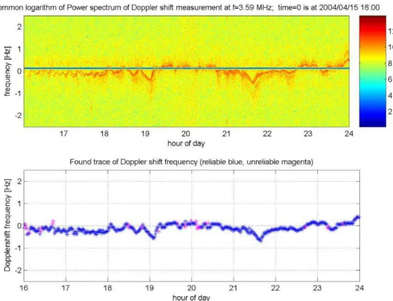
Fig. 1. An example of a Doppler record: the upper plot is the initial Doppler spectrogram, the lower plot represents a curve of Doppler
frequency shift corresponding to the spectral peak in the spectrogram found by special software. Blue colour depicts points of high reliability; the magenta colour depicts points of low reliability. Time is in UT.
this arrangement is a strong ground wave that makes the de-tection of small Doppler shift (∼ less than 0.04 Hz) impos-sible. We eliminate the signal corresponding to the ground wave by digital processing in the frequency domain. On the other hand, the ground wave provides us with direct verifica-tion of the stability of the oscillators and zero drift line.
Since we are using a frequency in the amateur band, we have to transmit a call sign each minute. The duration of the call sign is ∼5 s. During that time the data acquisition is stopped. That means that the maximum time interval that can be processed by the FFT algorithm is ∼55 s, so the best frequency resolution that we can obtain is ∼1/55=0.018 Hz. The receiver and transmitter are synchronised by GPS clock. The data are visualised by means of spectrograms, usually with a time resolution of 1 min.
The Doppler system has one more working frequency near 7.0 MHz. However, there are technical problems with high level of noise at this frequency and, moreover, it is suitable only during daytime and moderate and high solar activity conditions, not near the solar cycle minimum like in 2006, when foF2 is almost all the time below 7 MHz.
3 Comparison of phase paths calculated from iono-grams and Doppler records
A routine ionosonde measurement is usually repeated once every 15 min. To compare ionogram and Doppler measure-ments we selected 21 days, when there was only one trace or one trace clearly dominated on Doppler records (high quality data). As a result, we could detect a spectral peak and follow this peak from spectrum to spectrum. To present a detailed analysis of each of the 21 individual days would be boring for readers. Therefore, we present the comparative analysis only for nine representative days (41, 42, 68, 69, 93, 96, 106, 117, 149) of 2004. Figure 1 shows an example of such Doppler records during day 106 of 2004.
As mentioned above, routine N(h) profiles are processed from recorded ionograms automatically by the ARTIST soft-ware. However, the automatic scaling can sometimes be in-correct. Thus, we have manually tested and, when necessary, corrected the automatic scaling of all ionograms involved in this study. Phase paths have been computed using only N(h) profiles obtained from manually revised ionogram scaling. On the other hand, ionograms shown in the paper (Figs. 2 and 5–8) are digisonde-generated automatic scaling figures, used solely to detect intervals, when only ordinary trace, or
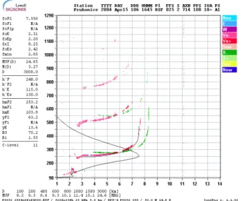
Fig. 2. An example of the ionogram recorded at Pruhonice at 16:45 UT of the day 106 of 2004, when only the O-trace marked by red colour was present in the vicinity of f=3.6 MHz.
only extraordinary trace, or sporadic E layer are present at ionograms.
There is an ambiguity in Doppler measurements since we are not sure what mode of wave (ordinary or extraordinary) we are observing on the Doppler records. To remove this ambiguity, we used the following approach:
1. We consider the presence or absence of O- (ordinary) and X- (extraordinary) echo traces near 3.6 MHz on ionograms. The absence of X-trace (O-trace) on iono-grams (see an example of such a case in Fig. 2) during some intervals allows us to claim that the Doppler sys-tem measures the O- trace (X-trace), that trace which is present at ionograms.
2. In the case where both O- and X-traces are present close to 3.6 MHz, we calculate Pc(t) (the phase path,
calcu-lated from the ionogram) for O-trace and for X-trace and compare the calculated phase paths with the exper-imental phase path Pe(t) obtained from Doppler
mea-surements for every interval. We calculate the average difference (m) based on squares of individual differ-ences between calculated and experimental phase paths. We use m to define what components, O- or X-echo traces, coincide in the best way with experimental one, and we suppose that this mode of wave is what we ob-serve on the Doppler records.
Figure 2 displays a gap in the record at 3.6 MHz as a conse-quence of interference with the Doppler system signal during common volume measurements. However, presence of only the O trace on ionogram at frequencies below and above the gap allows us to assume that only the O trace is present at
3.6 MHz. Similar gaps at 3.6 MHz are observed also at other ionograms shown in the paper – always for the same reason and without impact on our considerations and results.
Figures 3 and 4 present examples of typical results of com-parison of the calculated and experimental phase paths. 3.1 Day 149 of 2004 (Fig. 3a)
We observed only the O-trace on the ionograms in the re-gion nearby to 3.6 MHz from 04:45 to 05:00 UT and then from 15:45 to 17:00 UT. We used these intervals to deter-mine h0. A sporadic E-layer (Es) was present on the
iono-grams from 05:15 to 12:30 UT. Both O- and X-traces were recorded on the ionograms in the region close to 3.6 MHz from 00:15 to 04:45 UT. Comparing with the experimental phase path, the difference for the calculated phase paths for O-wave was m=7.6 km, while for X-wave m=18.2 km. Thus,
Pc(t ) of O-wave agrees better with the experiment. The
av-erage difference m is calculated as an avav-erage value from absolute values of differences (i.e. irrespective of their sign) between ionogram and Doppler phase paths. Thus small
m means good coincidence between phase paths. There is
a sharp shift of the experimental phase path from 05:00 to 05:15 UT, because the radio wave reflection point dropped from the F-layer to Es. There was an O-echo trace and Es
-trace on the ionograms close to 3.6 MHz from 12:45 to 15:30. The comparison of Pc(t) with Pe(t) shows m=8.2 km for
O-trace and m=5.4 km for the Es-trace in this interval. Thus,
Pc(t ) for the wave reflected from the Es layer agrees better
with the experiment. Another sharp shift of the experimental phase path was observed from 15:45 to 16:00 UT. In this case the radio wave reflection point jumped from Es to F layer.
Again, both O- and X-echo traces were present on the iono-grams in the vicinity of 3.6 MHz from 17:15 to 23:45 UT. The comparison of calculated phase path with experimental one reveals m=12 km for O-trace and m=5.5 km for X-trace. Thus, we consider Pc(t ) of X-trace to be closer to the
ex-perimental phase path. ARTIST does not take into account the sporadic E layer when computing electron density profile. Sporadic E layer was present on the ionograms from 05:15 to 15:30 UT, as illustrates an ionogram and corresponding N(h) profile shown in Fig. 5. As a result, the differences between
Pc(t ) for O-wave and Pe(t ) was m=11 km.
3.2 Day 106 of 2004 (Fig. 3b)
We saw a few intervals on ionograms, where only the O-trace in the region of 3.6 MHz was present. We used these inter-vals to define h0. The comparison of calculated phase paths
with experimental ones shows m=6.3 km and m=22.8 km for O-trace and X-trace, respectively. So, the Pc(t) calculated for
the O-trace shows better agreement with experimental phase paths Pe(t ). Some discrepancies between the phase paths
in the interval from 11:00 to 16:00 UT are caused by spo-radic E or by gaps in the trace on the ionogram (Fig. 6). It
D. Buresova et al.: Assessing the quality of ionogram interpretation using the HF Doppler technique 899 0 2 4 6 8 10 12 14 16 18 20 22 24 t, h 80 120 160 200 240 280 P , k m day 149, 2004 0 2 4 6 8 10 12 14 16 18 20 22 24 t, h 80 120 160 200 240 280 320 P , k m day 106, 2004 a b 0 2 4 6 8 10 12 14 16 18 20 22 24 t, h 100 150 200 250 300 350 P , k m 117 day 2004 Manual corrected scaling
of the ionograms 0 2 4 6 8 10 12 14 16 18 20 22 24 t, h 100 150 200 250 300 350 P , k m 117 day, 2004 Automatically scaled ionograms c d 0 2 4 6 8 10 12 14 16 18 20 22 24 t, h 80 120 160 200 240 280 P , k m 68 day, 2004 2 4 6 8 10 12 14 16 18 20 22 24 t, h 69 day, 2004 e f
Fig. 3. Typical phase paths of radio wave (f=3.6 MHz) calculated from ionogram (triangles) and inferred from Doppler records (full-circle
lines) for the days 68, 69, 106, 117 and 149 of 2004 involved in the study. Comparison of the Pc(t ) calculated from manually corrected and
automatically scaled ionograms with Pe(t ) are shown in the plots (c) and (d), respectively. Time is in UT.
is necessary to note that the day 106 was geomagnetically quiet day (Dst index was smaller than 11), the quality of the
recorded ionograms was high, and the manual correction of ionogram scaling practically not necessary.
3.3 Day 117 of 2004 (Figs. 3c, d)
On the Pruhonice digisonde records the O-trace dominated close to 3.6 MHz from 05:45 to 06:00. Well-developed Es-trace was observed during the intervals from 06:30 to
09:45 UT, from 12:45 to 14:30 UT, from 15:00 to 15:30 UT, and from 19:00 to 22:30. Both O- and X-echo traces were
2 4 6 8 10 12 14 16 18 20 22 24 t,h 0 2 4 6 8 10 12 14 16 18 20 22 24 t,h 100 150 200 250 300 350 P, k m 41 day, 2004 42 day, 2004 a b 2 4 6 8 10 12 14 16 18 20 22 24 t,h 0 2 4 6 8 10 12 14 16 18 20 22 24 t,h 100 150 200 250 300 350 P, k m 93 day, 2004 96 day, 2004 c d
Fig. 4. Typical phase paths of radio wave (f=3.6 MHz) calculated from ionogram (triangles) and inferred from Doppler records (full-circle
lines) for the days 41, 42, 93 and 96 of 2004 involved in the study. Time is in UT.
present on the ionograms close to 3.6 MHz from midnight to 05:30 UT. Comparing with Pe(t ), we obtained m=2.56 km
for Pc(t ) calculated for O-trace, and m=33.6 km for the phase
path calculated for X-trace within this time interval. Thus,
Pc(t ) of O-trace agrees better with the experimental Pe(t ).
There is an altitudinal significant shift of the experimen-tal phase path from 06:15 to 06:30 UT (Fig. 3c), probably caused by the movement of the radio wave reflection height from F layer to the Es layer. There were both ordinary and
extraordinary F layer traces and the trace of Es layer on the
ionograms close to 3.6 MHz from 15:45 to 16:15 UT. The comparison of Pc(t ) with Pe(t ) shows m=2.7 km for O-trace
and m=7.7 km for the Es-trace. Thus, Pc(t ) calculated for
O-trace displayed better agreement with the Pe(t ). Both O- and
X-traces were again observed on the ionograms in the vicin-ity of 3.6 MHz from 16:45 to 23:45 UT. The comparison of calculated phase paths with experimental ones showed better agreement for the Pc(t ) obtained for the ordinary trace. From
Fig. 3c it is evident that the discrepancy between Pc(t ) and
Pe(t ) is considerably higher during the time intervals from
06:30 to 15:45 UT and 19:00 to about 23:00, during the pe-riods when the Eslayer was present (examples of ionograms
are presented in Fig. 7). The above finding is valid for all analysed time periods, when Es layer occurred in the vicinity of 3.6 MHz. Furthermore, Fig. 3c shows the phase paths ob-tained from manually corrected ionograms; manual correc-tion removed outliers observed in uncorrected data (Fig. 3d) caused by automatic scaling. The average difference for au-toscaled data was m=9.4 km, while after correction it de-creased to m=7.8 km.
3.4 Day 68 of 2004 (Fig. 3e)
It was a quiet magnetic day: the Dst index was higher than
−6 nT. Again, to define h0, we selected the time intervals,
when only the O-trace was present close to 3.6 MHz. The X-trace dominated on ionograms from 00:15 to 05:00 UT.
D. Buresova et al.: Assessing the quality of ionogram interpretation using the HF Doppler technique 901
Fig. 5. An example of the ionogram recorded at Pruhonice
obser-vatory at 09:15 UT of the day 149 of 2004 when sporadic E was present. Black line shows the automatically scaled N(h) profile by the ARTIST software.
During this time period foF2 was less than 3.6 MHz and we got no required digisonde data. The comparison of calcu-lated phase paths with experimental ones for the time peri-ods, when both O- and X-traces were present on the iono-grams (e.g., from 05:15 to 06:30 UT), reveals m=16.2 km and m=4.3 km for O- and X-traces, respectively. Thus, Pc(t )
calculated for the X-trace agrees better with the Pe(t ). A
similar situation was observed for the period from 15:30 to 23:45 UT. The comparison of Pc(t ) with Pe(t ) exhibits
m=14.1 km for O-trace and m=5.4 km for X-trace in this
in-terval. Thus, Pc(t ) calculated for X-trace agrees better with
the experimental Pe(t ). The discrepancy between Pc(t ) and
Pe(t ), observed during the period from 06:45 to 16:00 UT,
could be attributed partially to the presence of gaps on the ionograms just above foE between the E and F layers, and partially to the affinity of foF2 layer to the working frequency of the Doppler apparatus. Examples of such ionograms are presented in Fig. 8. It is well known that regions of decreas-ing ionisation between the ionospheric layers do not reflect the radio waves and the resulting discontinuity leads to un-certainty in the true height above the valley region.
3.5 Day 69 of 2004 (Fig. 3f)
This day was one of the geomagnetically disturbed days (Dst
index started to decrease at noon and reached the minimum value of −71 nT at 23:00 UT). To define h0, we selected
the time intervals, when only the O-trace was present in the vicinity of 3.6 MHz. The X-trace of the ionospheric F2 layer dominated on the ionograms close to 3.6 MHz from 04:00 to 05:00 UT. As in the previous case, foF2 was less than 3.6 MHz during this period, and we have got no required
Fig. 6. An example of the ionogram recorded at Pruhonice
obser-vatory at 11:30 UT of the day 106, 2004, when O-trace was absent in the frequency range close to 3.6 MHz. Black line shows the au-tomatically scaled N(h) profile.
digisonde data. Then we separated the time periods when both O- and X-traces occurred on the ionograms nearby 3.6 MHz. After 22:15 UT, again, foF2 fell below 3.6 MHz, and only the X-trace was present on ionograms. That is why only Pe(t ) is plotted in the Fig. 3f after 22:15 UT. There is a
“jump” upward (about 40 km) of experimental and calculated phase paths from 18:00 to 18:15 (18:00 UT is shown by ver-tical dotted line in Fig. 3f). At this time Dst index dropped
below −50 nT.
We can also see large discrepancies between the phase paths (up to 40 km) after 18:00 UT. This could mean a prob-lem in ARTIST scaling (in its subprograms ARTNHPC used in ARTIST to invert scaled ionogram trace data into N(h) profiles working in real-time mode and JAVANHPC used in SAO Explorer) for geomagnetically disturbed ionosphere. Results of Chen et al. (1991, 1994) support this sugges-tion. They compared inverted N(h) profiles from digisonde ionograms recorded at Millstone Hill (42.6◦N, 284.5◦E) and Arecibo (18.5◦N, 292.◦9 E) stations with those obtained from incoherent scatter radar measurements. They showed that the probable reason for the occurrence of larger devia-tions under the geomagnetic storm condidevia-tions is inaccuracy within the valley model.
Another example of the geomagnetically disturbed day is day 42 of 2004 (Fig. 4b). This strong wintertime storm started at about 09:00 UT on day 42 and achieved its maxi-mum at 17:00 UT when the Dst index felt down to −109 nT.
Diurnal courses of the calculated and experimental phase paths obtained for the stormy day and for the preceding quite day of 10 February 2004 (day 41) are plotted in Figs. 4a and b. An X-trace was dominant during the night starting
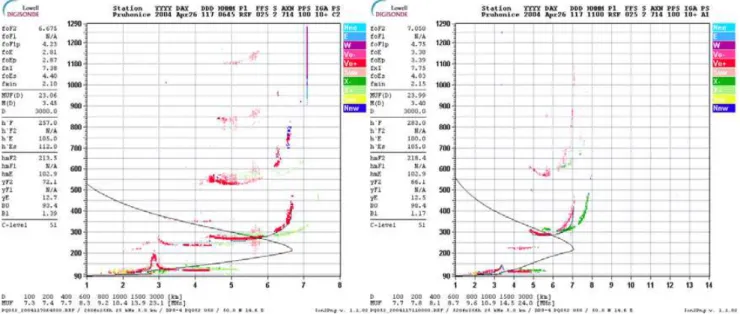
Fig. 7. Examples of ionograms recorded at Pruhonice observatory at 06:45 UT (left panel) and at 11:00 UT (right panel) for analysed day
117 of 2004, when sporadic E was present. Black line shows the automatically scaled N(h) profile.
Fig. 8. Examples of the ionograms recorded at Pruhonice observatory during the day 68 of 2004: (a) ionospheric E-layer and gap between
E and F layers; (b) affinity of critical frequency of F layer to the sounding frequency of the Doppler apparatus. Black line shows the automatically scaled N(h) profile. Time is in UT.
at about 17:00 UT till early morning hours (06:00 UT) dur-ing both 41 and 42 days. Durdur-ing several morndur-ing hours of day 41 and late evening hours of both analyzed days foF2 was below 3.6 MHz and we have got no ionosondes data. Discrepancies between Pc(t ) and Pe(t ) observed within the
period from about 07:00 UT to 16:00 UT on day 41 could be attributed to the presence of gaps on the ionograms just above foE between E and F layers. The gap in the diurnal course of Pe(t ) from 08:00 till 15:00 UT on day 42 is due
to a low quality of Doppler records. Significant differences between the both Pc(t ) and Pe(t ) phase paths appeared
af-ter 15:00 UT when Dst dropped below −50 nT (this time is
shown by vertical dotted line).
Day 96 of 2004 (Fig. 4d) was also a disturbed day. A moderate geomagnetic storm had its onset at about 08:00 UT. Between 17:00 UT and 18:00 UT the Dstbecame lower than
−50 nT. The storm culminated near 19:00 UT when the Dst
D. Buresova et al.: Assessing the quality of ionogram interpretation using the HF Doppler technique 903 from Doppler and digisonde records for the disturbed day 96
are compared with those obtained for quiet day 93 in Figs. 4c and d. During both 93 and 96 days the X-trace dominated during the night starting at about 19:00 UT. A sporadic E-layer was present on the ionograms during the day 93 from 11:00 to 12:15 UT. An appearance of the Es could be consid-ered as a cause of difference between Pc(t ) and Pe(t ) within
this time period. We have got no data till 04:45 UT for the stormy day because of low foF2. Beginning of the consid-erable discrepancies between phase paths (up to 37 km) we observed after 18:30 UT under storm conditions.
The fact that ARTIST is not very reliable under certain conditions (as any other autoscaling program) is well-known fact, at least in the European ionosonde community (e.g., Zolesi et al., 2004) in spite of the fact that ARTIST un-derwent several times modifications that improved the qual-ity of its analysis and its network-wide upgrade is under-way (Galkin et al., 2006). For this reason the European ionospheric project COST296 runs database of automatically scaled results (parameters, profiles), and separately database of manually checked results (parameters, profiles). Main problems appear at F1 region heights, maybe as a conse-quence of the E-F region valley influence. Our Doppler sounding frequency is very often reflected just at F1 region heights.
The days shown here are typical examples of the behaviour of the difference between the phase paths computed from ionograms and from the Doppler system measurements. We analysed more days, but we cannot present in one paper all days, this would make the paper long and boring.
We have been working with a frequency of 3.6 MHz, which is during daytime usually well below foF2. This means that we can often use Doppler system measurements to improve ionogram inversion into the electron density pro-file at heights well below the F2 region maximum and, thus, the effect of possible differences, formed in the height inter-val between the 3.6 MHz reflection height and hmF2, on the
hmF2 determination is not included.
4 Conclusions
The comparison of calculated Pc(t ) and experimental Pe(t )
phase paths for 21 selected days of 2004 allows us to estimate the magnitude of the difference between the values of the phase path obtained by the Digisonde Portable Sounder DPS-4 and the new Doppler type system during the common vol-ume measurements at European midlatitude station Pruhon-ice. To avoid additional inaccuracy, scaling of all ionograms obtained from DPS-4 was manually corrected. It is also im-portant to note that days of 2004 involved in the analysis were geomagnetically quiet days, except for days 42, 69 and 96, when moderate-to-intense storm conditions took place. The overall average difference between Pc(t ) and Pe(t ) is
m=11.1±1.2 km, standard deviation is 5.0 km. In the best
case the average daily difference was about 3 km, which is comparable with the height resolution of the digisonde mea-surements. The substantial disagreement between Pc(t ) and
Pe(t ) is obtained in three cases: (1) presence of Es layer,
(2) when the sounding frequency is close to the critical fre-quency of ionospheric layer, and (3) during geomagnetic storms (see Figs. 3f, 4b and d). On the other hand, during geomagnetically quiet days, absence of the sporadic E layer, and at availability of high quality ionograms and correct scal-ing, the electron density profiles, calculated by the Auto-matic Real Time Ionogram Scaler with True height algorithm (ARTIST) on the basis of such ionograms, can be considered reliable. Obviously the comparison of experimental and cal-culated phase paths can help to test the inversion codes of electron density profiles.
Acknowledgements. Authors acknowledge support by the grant
No. 205/04/2110 of the Grant Agency of the Czech Republic. Au-thors thank both referees for their helpful comments.
Topical Editor M. Pinnock thanks L.-A. McKinnell and another referee for their help in evaluating this paper.
References
Bibl, K.: Evolution of ionosonde, Annali di Geophys., 41(5–6), 667–680, 1998.
Bossy, L.: Accuracy comparison of ionogram inversion methods, Adv. Space Res., 14(12), 39–42, 1994.
Chen, C.-F., Ward, B. D., Reinisch, B. W., and Buonsanto, M. J.: Ionosonde observations of the E-F valley and comparison with incoherent scatter radar profiles, Adv. Space Res., 11(10), 89– 92, 1991.
Chen, C.-F., Reinisch, B. W., Scali, J. L., and Huang, X.: The accu-racy of ionogram-derived N(h) profiles, Adv. Space Res., 14(12), 43–46, 1994.
Davies, K.: Ionospheric radio waves, Blaisdell Publishing Com-pany. A Division of Ginn and Company, Waltham, Massachusetts – Toronto – London, 1969.
Galkin, I. A. and Dvinskikh, N. I.: Interpretation of vertical inci-dence sounding data by electronic computing machine BECM-2M (in Russian), Studies Geomagn. Aeronautic Phys., Sun 3 (part 1), 109–143, 1968.
Galkin, I. A., Khmyrov, G. M., Kozlov, A., Reinisch, B. W., Huang, X., and Kitrosser, D. F.: Ionosonde network-ing, databasnetwork-ing, and web servnetwork-ing, Radio Sci., 41(5), RS5S33, doi:10.1029/2005RS003384, 2006.
Paul, A. K.: Limitations and possible improvements of ionospheric models for radio propagation: Effects of sporadic E layers, Radio Sci., 21(3), 304–308, 1986.
Pezzopane, M. and Scotto, C.: The INGV software for the auto-matic scaling of foF2 and MUF(3000)F2 from ionograms: A performance comparison with ARTIST 4.01 from Roma data, J. Atmos. Sol.-Terr. Phys., 67, 1063–1073, 2005.
Reinisch, B. W. and Huang, X.: Automatic calculation of electron density profiles from digital ionograms, 3, Processing of botom-side ionograms, Radio Sci, 18, 477–492,1983.
Reinisch, B. W., Huang, X., Galkin, I. A., Paznukhov, V., and Ko-zlov, A.: Recent advances in real-time analysis of ionograms and
ionospheric drift measurements with digisondes, J. Atmos. Sol.-Terr. Phys., 67, 1054–1062, 2005.
Titheridge, J. E.: Starting models for the real height analysis of ionograms, J. Atmos. Sol.-Terr. Phys., 48, 435–446, 1986. Wright, J. W., Laird, A. R., Obitts, D., Violette, E. J., and McKinnis,
D.: Automatic N(h,t) profiles of the ionosphere with a digital ionosonde, Radio Sci., 7, 1033–1043, 1972.
Zolesi, B., Belehaki, A., Tsagouri, I., and Cander, L. R.: Real-time updating of the Simplified Ionospheric Regional Model for operational applications, Radio Sci., 39, RS2011, doi:10.1029/2003RS002936, 2004.