HAL Id: hal-00316896
https://hal.archives-ouvertes.fr/hal-00316896
Submitted on 1 Jan 2001
HAL is a multi-disciplinary open access
archive for the deposit and dissemination of
sci-entific research documents, whether they are
pub-lished or not. The documents may come from
teaching and research institutions in France or
abroad, or from public or private research centers.
L’archive ouverte pluridisciplinaire HAL, est
destinée au dépôt et à la diffusion de documents
scientifiques de niveau recherche, publiés ou non,
émanant des établissements d’enseignement et de
recherche français ou étrangers, des laboratoires
publics ou privés.
Mean winds observed with Indian MST radar over
tropical mesosphere and comparison with various
techniques
M. Venkat Ratnam, D. Narayana Rao, T. Narayana Rao, S. Thulasiraman, J.
B. Nee, S. Gurubaran, R. Rajaram
To cite this version:
M. Venkat Ratnam, D. Narayana Rao, T. Narayana Rao, S. Thulasiraman, J. B. Nee, et al..
Mean winds observed with Indian MST radar over tropical mesosphere and comparison with
var-ious techniques. Annales Geophysicae, European Geosciences Union, 2001, 19 (8), pp.1027-1038.
�hal-00316896�
Annales
Geophysicae
Mean winds observed with Indian MST radar over tropical
mesosphere and comparison with various techniques
M. Venkat Ratnam1, D. Narayana Rao1, T. Narayana Rao1, S. Thulasiraman2, J. B. Nee2, S. Gurubaran3, and R. Rajaram3
1Department of Physics, S. V. University, Tirupati – 517 502, India
2Department of Physics, National Central University, Chung Li, 32054, Taiwan
3Equatorial Geophysical Research Laboratory, Indian Institute of Geomagnetism, Tirunelveli, India
Received: 15 November 2000 – Revised: 9 April 2001 – Accepted: 20 April 2001
Abstract. Temporal variation of mean winds between the 65 to 85 km height region from the data collected over the course of approximately four years (1995–99), using the In-dian MST radar located at Gadanki (13.5◦ N, 79.2◦E),
In-dia is presented in this paper. Mesospheric mean winds and their seasonal variation in the horizontal and vertical com-ponents are presented in detail. Westward flows during each of the equinoxes and eastward flows during the solstices are observed in the zonal component. The features of the semi-annual oscillation (SAO) and the quasi-biennial oscillation (QBO) in the zonal component are noted. In the meridional component, contours reveal a northward motion during the winter and a southward motion during the summer. Large inter-annual variability is found in the vertical component with magnitudes of the order of ±2 ms−1. The MST ob-served winds are also compared with the winds obob-served by the MF radar located at Tirunelveli (8.7◦ N, 77.8◦ E), In-dia, the High Resolution Doppler Imager (HRDI) onboard the Upper Atmospheric Research Satellite (UARS), and with the CIRA-86 model. A very good agreement is found be-tween both the ground-based instruments (MST radar and MF radar) in the zonal component and there are few discrep-ancies in the meridional component. UARS/HRDI observed winds usually have larger magnitudes than the ground-based mean winds. Comparison of the MST derived winds with the CIRA-86 model in the zonal component shows that during the spring equinox and the summer, the winds agree fairly well, but there are a lot of discrepancies in the other seasons and the observed winds with the MST radar are less in mag-nitude, though the direction is same. The strengths and limi-tations in estimating reliable mesospheric mean winds using Correspondence to: D. N. Rao ([email protected])
the MST radar are also discussed.
Key words. Meteorology and atmospheric dynamics (gen-eral circulation; middle atmosphere dynamics; waves and tides)
1 Introduction
During the past decade remarkable advances have been made in our understanding of the dynamics of the equatorial meso-sphere. The low latitude mesosphere is characterized by a variety of dynamical processes, some of which are confined only to this region. The global circulation at these heights is not well-known at low latitudes where the Coriolis pa-rameter is weak. As a result, relatively long period waves, such as Kelvin and mixed Rossby gravity waves exist in this region (Vincent, 1993; Eckermann et al., 1997). The dy-namics of the equatorial atmosphere is strongly controlled by the evolution and breakdown of these waves (Balsley and Gage, 1980; Balsley, 1983; Muraoka et al., 1989). A vari-ety of experimental techniques, which includes radars (MF, Meteor, VHF) (Vincent and Lesicar, 1991; Raghava Reddi and Ramkumar, 1995; Nakamura et al., 1996), a satellite born Limb Infrared Monitor of the stratosphere (LIMS) ex-periment which covers the lower mesosphere (Salby et al., 1984), High Resolution Doppler Imager (HRDI) on the Up-per Atmospheric Research Satellite (UARS) (Burrage et al., 1996), the COSPAR International Reference Model (CIRA 86) (Barnett and Corney, 1985), etc. have evolved, each hav-ing their own limitations, to study global climatology of the winds and waves in the mesosphere. Among them, the VHF radar plays a unique role in understanding the dynamics of
1028 M. V. Ratnam et al.: Mean winds over tropical mesosphere 26 July 1999 Figure 1 -60 -45 -30 -15 0 -20-10 0 10 -2 -1 0 1 2 W (ms-1) v (ms-1) u (ms-1 ) East West Zenith Y North South
Fig. 1. Averaged Doppler spectra recorded on 26 July 1999 at around 1030 LT in different beam directions showing the echo characteristics
at different height regions in the mesosphere. Right panel of figure shows the estimated vertical and horizontal winds.
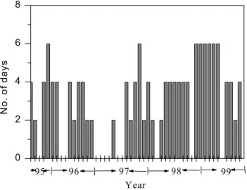
0 2 4 6 8 Figure 2 Year 95 96 97 98 99 N o . o f d a y s
Fig. 2. Number of days of the Indian MST radar data used for this
study for each month from September 1995 to August 1999.
the mesosphere for their better temporal and altitude reso-lution (Woodman and Guillen, 1974). Both Meteor and MF radars are widely used to measure the mesospheric and lower thermospheric motions (Vincent, 1993; Raghava Reddi and Ramkumar, 1997; Rajaram and Gurubaran, 1998). These radars have the capability to monitor the Mesosphere and Lower Thermosphere (MLT) winds on a continuous basis, but are more reliable above 80 km. The model (CIRA 86) derived winds are primarily based on rocket and satellite ob-servations and are not suitable for all latitudes (Manson et al., 1991) especially in the tropics (Hedin et al., 1996). But MST radar can be effectively used to overcome the difficulties of the other techniques, especially in the 65–85 km height re-gion inspite of some limitations. These limitations will be discussed in detail in Sect. 3. The network of point observa-tions would be highly complementary for the existing satel-lite and model database, which provides gross features of the geostropic wind field and other parameters on a global scale. In this regard, MST radar observations can provide valuable complementary information on winds at these lower heights (R¨ottger et al., 1983).
2 System description and database
The Indian MST radar is a very high power monostatic co-herent pulsed Doppler radar operating at 53 MHz with a peak power aperture product of 3 × 10¹⁰Wm2and it is located at Gadanki (13.5◦N, 79.2◦E), a tropical station in India. The
antenna system occupying an area of 130 m × 130 m is a phased array of 32 × 32 three element Yagi antennas consist-ing of two orthogonal sets, one for each polarization (mag-netic E-W and N-S). It generates a radiation pattern with the side lobe level of −20 dB. The main beam can be positioned at any look angle within ±20◦ off zenith in the two major planes (E-W and N-S) with 1◦interval. The number of FFT points are up to 512 and coherent integrations are from 4 to 512 (selectable in binary steps). The uncoded pulse widths can be from 1µs – 32µs (in binary steps) and the coded ones, 16µs and 32µs with 1µs baud length. Details of the sys-tem description are given by Rao et al. (1995) and Kishore (1995).
For the present study, in order to measure the three com-ponents of wind velocity in the mesosphere, the main beam of the MST radar is oriented in the vertical and four off-vertical (E 10◦, W 10◦, N 10◦ and S 10◦) directions. The received echo signals were sampled at intervals of 1.2 km in the height range of 65–85 km and were coherently integrated over 64 pulses of transmission. The complete time series of the decoded and integrated signal samples are subjected to FFT for the on-line computation of the Doppler power tra for each range bin. Figure 1 shows a typical Doppler spec-tra recorded on 26 July 1999 in five different beam directions. This figure is the average of four spectra in a time span of 15 minutes at around 1030 LT (Local Time). The off-line data processing for the parameterization of the Doppler spectrum involves removal of dc, estimation of average noise level, in-coherent integration and computation of the three low radar moments. For estimating the average noise level, an objec-tive method developed by Hildebrand and Sekhon (1974) has been adopted here. The determined noise level is subtracted from the received power for each Doppler bin. The echoes due to meteor trails, which were detected less frequently, have been removed and the radial wind velocities are
esti-70 75 80 85 -30 -15 0 15 30 He ig h t ( k m) -30 -15 0 15 30 -30 -15 0 15 30 -30 -15 0 15 30 18 Sep 1996 28 Jun 1996 28 Mar 1996 21 Dec 1995 Meridional Zonal M ST radar PR radar 70 75 80 85 -20 -10 0 10 20 He ig h t ( k m) Velocity (ms-1 ) -20 -10 0 10 20 -20 -10 0 10 20 -20 -10 0 10 20 Q M
Fig. 3. Comparison of mean zonal and
meridional winds between the MF and MST radars on individual days in dif-ferent seasons.
mated using a non-linear, least square fitting method of the Doppler shifted spectrum. Since the radar echoes at meso-spheric heights are highly intermittent in space and time and since turbulence occurs in the form of layers rather than con-tinuously, we have adopted a different method for estimating winds, which is given in the Appendix. The right-hand panel in Fig. 1 shows the typical wind velocities observed at the same time. As seen in Fig. 1, westward velocity of the order of 50 m s−1, equatorward velocity of the order of 20 m s−1 and vertical velocity of the order of ±2 m s−1 are observed in the zonal, meridional and vertical velocities, respectively.
The database used for the present study is shown in Fig. 2. An average of four days of data per month are available. The Indian MST radar is operated in two schedules. In the first schedule, the radar is operated continuously from 1030 to 1630 LT and in the other schedule, the radar is operated for about 20 minutes every hour, starting from 1000 LT until the next day at 1000 LT. Four years of Indian MST radar data, starting from September 1995 to August 1999, were utilized for the study of mean and seasonal variations in the hori-zontal and vertical winds over Gadanki. Simultaneous ob-servations of the horizontal winds measured at Tirunelveli (8.7◦ N, 77.8◦E) using MF radar and velocities estimated by UARS/ HRDI for the above-mentioned period are also used in the present study. Before going into the results of the MST radar observed winds and their comparison with various techniques, systematic errors in estimating the winds using the MST radar technique are first discussed below.
3 Strengths and limitations of VHF radar measurements of mesospheric winds
The strengths and limitations of MST radar measurements of mesospheric winds have been discussed in detail by sev-eral authors (see R¨ottger et al., 1983; Nakamura et al., 1996;
Hocking, 1997; Namboothiri et al., 1999). Since the meso-spheric echoes are greatly influenced by the presence of elec-tron density fluctuations, which are prominent during day, radar observation is confined to daytime only. This involves the difficulty of performing harmonic analysis to deduce di-urnal and semididi-urnal components. We have used a simple averaging of daytime wind velocity, which is widely used as the mean wind estimation for the Indian MST radar. By using this simple averaging, the observed winds may be bi-ased by any existing diurnal variations. To estimate the bias induced by tidal components in the averaging processes (be-tween the daytime average wind and the 24 hour average), we have used amplitudes and phases observed with the MF Radar located at Tirunelveli at the lowest possible height, namely 84 km (below this height, measurements for all 24 hours are not available). The bias was primarily found in the range of 5–7.5 m s−1 at a height of 84 km. This bias may be smaller at the lower heights since the tidal ampli-tudes are usually smaller at lower heights (Nakamura et al., 1996). Thus, the daytime winds can be used to obtain mean winds over Gadanki.
Another limitation is that the turbulence is not uniformly distributed over the entire mesosphere, but rather it occurs in the form of layers. Moreover, the echoes are highly intermit-tent in space and time. These echoes are confined to a few kilometers primarily in the 70–80 km height region. Only in a few cases did the echoes appear to occur in the entire alti-tude region between 65 and 85 km. From Fig. 1, it is clear that strong echoes can be seen from 68 and 85 km, except at 73 km and 80 km. In this case, it is difficult to give the vertical profile of the winds. To overcome this difficulty, we have adopted a method described in detail in the Appendix. In brief, we have determined horizontal and vertical winds from the Doppler spectra if the signal-to-noise ratio (SNR) exceeded −14 dB. After subjecting the data to this
thresh-1030 M. V. Ratnam et al.: Mean winds over tropical mesosphere
MST Radar PR Radar
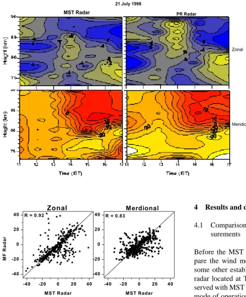
21 July 1998
Zonal
Meridional
Fig. 4. Contours showing the day-time
variations of the zonal and meridional winds as a function of altitude and the local time observed by the Indian MST radar and MF radar on 21 July 1999.
-40 -20 0 20 40 -40 -20 0 20 40 R = 0.92 MF R a d a r MST Radar -40 -20 0 20 40 -40 -20 0 20 40 Figure 5 R = 0.83 Merdional Zonal MST Radar
Fig. 5. Scatter plots of the winds in the altitude region of 65–85 km
for the zonal and meridional components using 60 coincidences of the MF and MST radar.
old, it was determined that at some range bins backscattered echoes are missing. For these cases, the procedure discussed in the Appendix is adopted. One more limitation is that the observations are limited on average for about four days in a month. Mean winds deduced by averaging for limited days do not always represent the seasonal variation of the mean wind. To overcome this problem, we have averaged the data collected with the Indian MST radar for about four years to obtain meaningful results on the seasonal variation of the mean winds. Aside from these limitations, MST radar has several advantages over other techniques. MST radar mea-surements have sufficient a signal-to-noise ratio in the height region of 65–85 km, which is not covered by the meteor radars. In this regard, it is worth having MST radar obser-vations as useful complementary information on the winds at these lower heights (R¨ottger, 1980; R¨ottger et al., 1981; R¨ottger et al., 1983).
4 Results and discussion
4.1 Comparison between MST and MF Radar wind mea-surements
Before the MST radar data is used, it is desirable to com-pare the wind measurements with the winds measured by some other established technique. Winds observed by MF radar located at Tirunelveli are used to compare winds ob-served with MST radar. Details of the system description and mode of operation of the MF radar can be found in Vincent and Lesicar (1991) and Rajaram and Gurubaran (1998). The data corresponding to the same day and same time (between 1000 LT to 1700 LT) have been collected from the MST and MF radars’ database. Figure 3 depicts a comparison be-tween the MST radar and the MF radar measured mean zonal and meridional winds on the individual days (these days are chosen randomly, very close to equinoxes and solstices) in four different seasons. In these figures and throughout the paper, a positive zonal wind is eastward, while a positive meridional wind is northward. Since the local time differ-ence between the stations is small, if the dynamical influ-ence is purely tidal, the two techniques will resolve the same structure. Clearly, excellent agreement can be seen in the zonal component for all the days, whereas some discrepan-cies are seen in the meridional component, especially dur-ing equinoxes. These variations in the meridional component might be due to other phenomenon dependent on the latitude and longitudinal structure of the tides, non-migrating tides and planetary waves.
Hourly averaged profiles of zonal and meridional wind ve-locities have been collected from both sites and Fig. 4 shows the typical daytime variations of zonal and meridional winds from 1100 LT to 1700 LT between the MST radar (left panel)
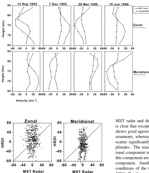
65 70 75 80 85 -60 -30 0 30 60 10 Jun 1998 28 Mar 1996 7 Dec 1995 13 Sep 1995 Meridional Zonal H e ig h t ( k m ) -60 -30 0 30 60-60 -30 0 30 60-60 -30 0 30 60 M ST radar U AR S/HRDI 65 70 75 80 85 -60 -30 0 30 60 Velocity (ms-1 ) H e ig h t ( k m )
-60 -30 0 30 60-60 -30 0 30 60-60 -30 0 30 60 Fig. 6. Same as Fig. 3 between the MST
radar and the UARS/HRDI for the alti-tude range of 65–85 km. -80 -40 0 40 80 -80 -40 0 40 80 Meridional Zonal MST Radar HR DI -80 -40 0 40 80 -80 -40 0 40 80 Figure 7 HR DI MST Radar Fig. 7. Scatter plots of the winds in the altitude region of 65–85 km
for the zonal and meridional components using 30 coincidences of the MST radar and the UARS/HRDI.
and the MF radar (right panel). A very good comparison in both the zonal (below 85 km) and meridional components is found between the two radar measurements in this case. From the figure, it is clear that between 76 and 85 km, the zonal wind is eastward and meridional wind is southward during the morning hours. At noon, the zonal wind has be-come westwards and in the evening, it is westward below 82 km and eastward above it. In the meridional component, the wind is still southward below 82 km and changes to north-ward above this height region. Here it should be noted that this is one of the best examples in which a good compari-son is found and on a few days, these two techniques yield rather poor agreement. We have collected about 60 simul-taneous observations of wind from the MST radar and the MF radar observations during 1995–1999. We have taken the hourly average values between 1100 LT to 1700 LT from both the radar data sets for a particular day. Figure 5 shows the scattered plots between the amplitudes measured by the
MST radar and the MF radar winds. From this figure, it is clear that except for the few cases, the zonal component shows good agreement between these two ground-based in-struments, whereas in the case of the meridional wind, the scatter significantly reveals larger discrepancies in the am-plitudes. The reason for the poor agreement in the merid-ional component might be due to the fact that the winds for this component are generally smaller than those for the zonal component. Another reason might be due to the sampling conditions of the two different techniques (Burrage et al., 1996). But the results presented here indicate that the merid-ional winds are not much smaller than those of the zonal winds. In fact, long temporal averaging of the data may dampen the amplitude of the tidal waves, while the latitudinal gradients in the tides may constitute a problem due to large separation (about 500 km in this case). This effect would be more for the meridional component since the tidal winds are stronger in the meridional component than in the zonal component.
4.2 Comparison between MST and UARS/HRDI wind mea-surements
We have also carried out a comparison of the MST radar wind measurements with the data obtained from the High Resolution Doppler Imager (HRDI) data. It is well-known that HRDI is designed to measure the horizontal winds in the mesosphere and the lower thermosphere, as part of the coordinated mission, which is aimed to improve the under-standing of the global climatology and atmospheric change (Reber et al., 1993). HRDI system details are available from Hays et al. (1993) and the wind deriving methodology is found in Burrage et al. (1996). We have chosen the near-est latitude (±2◦) and longitude (±20◦) data available from the HRDI in conjunction with the MST radar measurement
1032 M. V. Ratnam et al.: Mean winds over tropical mesosphere 65 70 75 80 85 -30 0 30
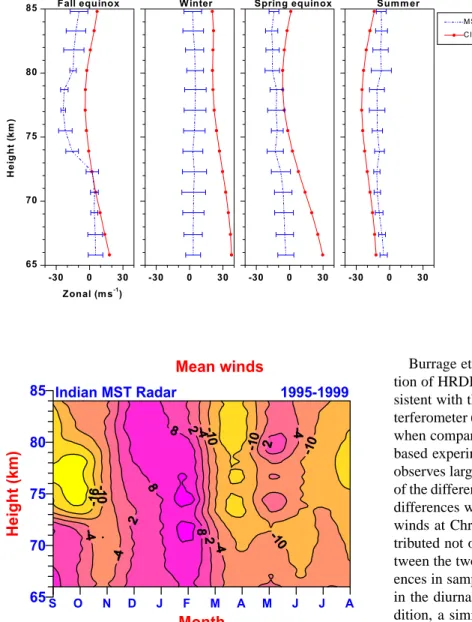
Fall equinox W inter Spring equinox Summ er
Zonal (m s-1 ) H e ig h t (k m ) -30 0 30 -30 0 30 -30 0 30 Figure 8 MST radar CIRA 86
Fig. 8. Comparison between the
CIRA-86 model values and the MST radar mean winds in the zonal component in different seasons.
Month
65 70 75 80 85He
igh
t (k
m)
S O N D J F M A M J J A Indian MST Radar 1995-1999Mean winds
Figure 9Fig. 9. Monthly mean zonal winds observed with the Indian MST
radar during 1995–1999. The dark shaded area corresponds to the eastward winds.
days and data for about 30 days of coincidence are available. Figure 6 shows the comparison between the MST radar and HRDI data on individual days in different seasons. Again, these days are selected in random very close to the equinoxes and solstices. From Fig. 6, it is clear that both the zonal and meridional components measured by the HRDI show larger values when compared to the MST data, but the di-rection (trend) of both of the components remains same, ex-cept on 10 June 1998. This can be more clearly seen from Fig. 7 which depicts the relationship between the amplitudes measured by the HRDI and MST radar measured horizontal winds for about 30 coincidences. In this case, the HRDI wind magnitudes are clearly much larger than those of the radar for both the components in this tropical station. A through examination of the comparisons between individual profiles has shown that the directions are the same.
Burrage et al. (1996) made a detailed study of the valida-tion of HRDI winds and found that the winds are more con-sistent with the rocket measurements and Wind Imaging In-terferometer (WINDII). But HRDI winds show discrepancies when compared to the winds obtained from various ground-based experiments. The main discrepancy is that the HRDI observes larger winds than the MF radars, but the magnitude of the difference varies between the various locations. Larger differences were observed between the HRDI and MF radar winds at Christmas Island (2◦N, 157◦W) and this was at-tributed not only to the problem of spatial displacement be-tween the two techniques, but also to the exacerbated differ-ences in sampling at the equator, where horizontal gradients in the diurnal tidal perturbations are at a maximum. In ad-dition, a similar but smaller discrepancy is found when the HRDI is compared to the Hawaii (22◦N) and Saskatoon (52◦
N) MF radars and this was partly attributed to the radar data analysis. Therefore, it seems that the HRDI winds are usu-ally large when compared to the ground-based measurements at the equator and low latitudes. Since Gadanki is also a low latitude station and the MST radar also has some limitations in its wind estimation method, we observe low values when compared to the HRDI winds. Burrage et al. (1996) pointed out that one of the reasons for this difference might be that the ground-based instruments provide the wind information directly above the station, whereas satellite born measure-ments provide the weighted average winds along the line-of-sight. We are planning to evaluate a detailed long-term aver-age picture of the winds using the HRDI data and compare it to the MST and MF radar observed wind climatology. 4.3 Comparison between MST radar and CIRA 86 model
winds
The MST radar observations have also been compared to the data obtained from the COSPAR International Reference Atmosphere (CIRA-86) model, which contains the monthly
65 70 75 80 85 -30 -20 -10 0 10 20 30 Fall equinox He ig h t ( k m ) -15 -10 -5 0 5 10 15 Winter 1995-1996 1996-1997 1997-1998 1998-1999 65 70 75 80 85 -20 -10 0 10 20 Spring equinox He ig h t ( k m) Zonal wind (ms-1 ) -20 -15 -10 -5 0 5 10 15 20 Figure 10 Summer
Fig. 10. Vertical profiles of mean zonal
winds over Gadanki during four sea-sons. The positive velocities corre-spond to an eastward flow.
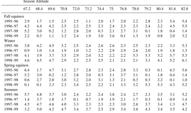
Table 1. Overall standard deviations for zonal wind
Season Altitude 67.2 68.4 69.6 70.8 72.0 73.2 74.4 75. 76.8 78.0 79.2 80.4 81.6 82.8 Fall equinox 1995–96 2.9 1.7 1.5 2.5 2.5 1.1 2.0 1.7 2.0 2.2 2.8 2.3 5.4 5.4 1996–97 4.2 4.4 4.2 2.5 2.2 2.5 2.3 2.4 2.3 2.3 2.4 2.2 4.5 5.5 1997–98 5.2 3.0 0.2 1.2 2.8 2.0 0.3 2.1 2.7 3.1 0.1 1.8 0.4 1.4 1998–99 2.2 0.3 1.1 3.3 2.4 1.9 3.0 3.6 0.1 1.3 1.9 0.8 2.0 3.2 Winter 1995–96 3.8 4.2 4.5 3.2 2.5 2.4 2.6 2.6 2.3 2.5 2.3 2.2 3.3 5.3 1996–97 0.9 1.0 1.4 1.9 1.0 1.2 2.2 2.9 2.9 2.6 2.0 1.9 1.8 1.3 1997–98 4.1 3.9 3.7 3.5 2.9 2.0 3.2 2.2 2.2 5.3 5.3 5.2 5.7 5.3 1998–99 4.6 4.5 4.7 2.9 2.2 2.5 2.5 2.1 2.1 2.1 3.1 4.1 5.2 6.1 Spring equinox 1995–96 6.4 1.7 4.7 3.1 2.7 2.8 2.3 2.4 2.8 3.3 0.3 0.1 6.3 5.6 1996–97 5.2 3.0 0.2 1.2 2.8 2.0 0.3 3.1 3.7 3.1 0.1 1.8 0.4 1.4 1997–98 0.6 2.7 2.0 3.0 3.2 2.0 3.1 1.3 2.1 0.3 0.3 2.2 0.1 1.0 1998–99 0.1 0.1 2.3 2.3 3.4 2.5 2.2 2.1 3.3 3.2 5.3 5.3 4.3 5.2 Summer 1995–96 5.7 4.8 3.7 3.0 2.4 2.2 2.4 3.8 2.4 2.7 2.3 3.5 3.1 5.2 1996–97 1.4 3.7 1.8 1.7 0.1 0.7 1.9 1.9 2.1 1.7 0.3 0.1 0.9 1.4 1997–98 4.5 4.7 4.6 4.0 3.3 2.3 2.3 2.3 3.0 2.6 3.7 3.4 1.3 4.7 1998–99 3.2 5.0 4.2 4.7 3.4 3.7 2.5 2.9 3.4 3.6 4.3 3.4 3.5 4.2
tabulations of the zonal mean wind from the ground to 120 km height region. This model contains the global gradient winds derived from the Nimbus 5 and 6 satellite radiance data in the altitude range of 20–80 km, and the MSIS-83 (Hedin, 1983) satellite and ground-based data in the altitude range of 80–120 km (Burrage et al., 1996). Figure 8 shows the comparison between the CIRA 86 winds and the MST radar
measured winds in the zonal component in four different sea-sons, i.e. spring equinox (Sep–Oct), winter (Nov–Feb), fall equinox (Mar–Apr) and summer (May–Aug). The four sea-sons presented here represent the average of the four years. Model values show larger amplitudes in all the seasons ex-cept in the fall equinox, where high magnitudes are observed in the MST radar observations. Manson et al. (1991) also
no-1034 M. V. Ratnam et al.: Mean winds over tropical mesosphere
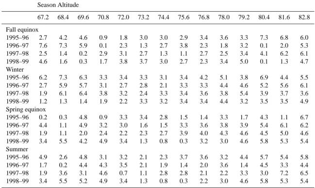
Table 2. Overall standard deviations for meridional wind
Season Altitude 67.2 68.4 69.6 70.8 72.0 73.2 74.4 75.6 76.8 78.0 79.2 80.4 81.6 82.8 Fall equinox 1995–96 2.7 4.2 4.6 0.9 1.8 3.0 3.0 2.9 3.4 3.6 3.3 7.3 6.8 6.0 1996–97 7.6 7.3 5.9 0.1 2.3 1.3 2.7 3.8 2.3 1.8 3.2 0.1 2.0 5.3 1997–98 2.5 1.4 0.2 2.9 3.1 2.7 1.3 1.1 2.7 2.5 3.4 4.1 6.2 6.1 1998–99 4.6 1.6 0.3 1.7 3.8 3.7 3.0 2.7 2.3 3.4 5.0 0.1 1.3 4.7 Winter 1995–96 6.2 7.3 6.3 3.3 3.4 3.3 3.1 3.4 4.2 5.1 3.8 6.9 4.4 5.5 1996–97 2.7 5.9 5.7 3.1 2.7 2.8 2.1 3.3 3.3 4.4 4.6 5.2 5.6 6.1 1997–98 1.9 6.1 6.4 3.8 3.2 2.4 3.3 3.4 3.6 3.8 5.4 3.9 3.7 3.6 1998–99 1.2 1.3 1.4 1.9 2.2 3.3 3.2 3.4 3.4 4.4 3.2 3.5 3.5 4.9 Spring equinox 1995–96 0.2 0.3 4.8 0.9 3.3 3.4 2.8 1.5 1.4 3.3 1.7 4.3 1.1 6.7 1996–97 4.4 1.1 4.9 3.2 3.0 1.6 1.5 3.3 3.6 3.8 3.9 5.4 6.1 6.2 1997–98 1.9 1.1 2.0 2.4 2.2 2.3 2.7 3.9 4.0 4.3 4.6 4.5 5.0 4.6 1998–99 3.4 5.5 4.2 4.9 3.4 1.3 0.8 0.3 3.2 3.0 4.6 5.8 5.3 5.4 Summer 1995–96 4.9 2.6 4.8 3.1 3.2 2.1 2.3 3.7 3.6 3.2 4.4 5.7 5.4 5.8 1996–97 1.7 0.2 4.4 4.3 3.5 2.1 1.9 1.4 2.0 3.6 1.4 4.5 3.3 4.4 1997–98 1.9 3.6 3.1 4.6 0.7 1.1 2.8 2.8 2.1 2.2 3.3 3.0 7.2 6.5 1998–99 3.4 5.5 5.2 4.9 3.4 1.3 0.8 0.3 2.2 3.0 4.6 5.8 5.3 5.4 Month 70 75 80 Heigh t ( km) Indian MST Radar 1995-1999 Figure 11
Fig. 11. Monthly mean meridional winds observed with the Indian
MST radar during 1995–1999. The dark shaded area corresponds to a northward flow.
ticed this type of discrepancy between radar measurements and winds derived from the CIRA-86 model. Nevertheless, a close examination of the comparisons between the individual profiles has demonstrated that the directions are in agreement similar to the HRDI. At low latitudes, both model values and satellite-derived winds are usually observed with large mag-nitudes than the winds derived from the ground-based instru-ments, as reported by several authors (Manson et al., 1991; Burrage et al., 1996).
5 Mean winds observed with the Indian MST radar As discussed in the earlier sections, it is observed that at low latitudes, both model values and satellite-derived winds are usually showing the larger magnitudes than the ground-based instruments (MST and MF radars). The daytime hourly val-ues derived from the MST radar observations on each day have been averaged in order to obtain the monthly values which, in turn, have been averaged for about four years. Fi-nally, the mean winds in both the zonal and meridional com-ponents are estimated. The main advantage of the MST radar over the other techniques is that it can give reliable verti-cal wind values as well. The long-term behavior of all three components of the winds is studied in detail and the results are presented in the following sections.
5.1 Zonal winds
The annual variation of the mean zonal winds obtained by the Indian MST radar is shown in Fig. 9. These values are the average of four years worth of data with the corresponding months averaged. Contours with positive values (dark shad-ing) represent the eastward component in the zonal winds. An eastward regime begins during the month of November and the flow becomes westward during the month of March. As can be seen from the figure, there has been a westward flow observed during each of the equinoxes, with eastward flows observed during the solstices. Similar results were re-ported by Rajaram and Gurubaran (1998) using the MF radar data at Tirunelveli (8.7◦ N, 77.8◦ E), which is the closest ground-based observing location. These results are
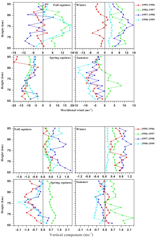
consis-65 70 75 80 85 -18 -12 -6 0 6 12 18 Fall equinox He ig h t ( k m ) -16 -12 -8 -4 0 4 8 12 16 W inter 1995-1996 1996-1997 1997-1998 1998-1999 65 70 75 80 85 -20 -15 -10 -5 0 5 10 15 20 Figure 12 Spring equinox He ig h t ( k m) Meridional wind (ms-1 ) -15 -10 -5 0 5 10 15 Summer
Fig. 12. Same as Fig. 10 but for the
meridional component. The positive velocities correspond to a northward flow. 65 70 75 80 85 -1.8 -1.2 -0.6 0.0 0.6 1.2 1.8 Fall equinox He ig h t ( k m ) -1.2 -0.8 -0.4 0.0 0.4 0.8 1.2 1995-1996 1996-1997 1997-1998 1998-1999 W inter 65 70 75 80 85 -2.1 -1.4 -0.7 0.0 0.7 1.4 2.1 Spring equinox He ig h t ( k m) Vertical component (ms-1 ) -2.1 -1.4 -0.7 0.0 0.7 1.4 2.1 Figure 13 Summer
Fig. 13. Same as Fig. 10 but for the
ver-tical component. The positive velocities correspond to an upward flow.
tent with those observed at Christmas Island (2◦N, 157◦W) using the Meteor radar (Avery et al., 1990) and MF radar (Vincent and Lesicar, 1991). The contours also clearly reveal a slight downward trend. The downward phase propagation is not as rapid as that observed by Vincent (1993), Vincent and Lesicar (1991) (1 km per day), Rajaram and Gurubaran (1998) (5.5 km per month) in the tropical latitudes. More-over, the westward flow during the fall equinox is stronger than that observed during the spring equinox in contrast to their observations. Although these two features are not that
much predominant, the zonal winds show a clear semiannual oscillation (SAO) which is predominant in the tropical lati-tudes.
The inter-annual variations of the mean zonal winds for the four seasons (spring and fall equinoxes, winter and sum-mer solstices) are shown in Fig. 10. The standard deviation observed while averaging seasonally is depicted in Table 1. From the table it is clear that the maximum error observed is less than 4 m s−1between the 70 and 80 km height region, while both above and below, the maximum error observed is
1036 M. V. Ratnam et al.: Mean winds over tropical mesosphere
≈6 m s−1, which implies that the MST radar observations in
the region of 70–80 km are more reliable. From Fig. 10, it is clear that the altitude dependence of the zonal winds for all seasons is consistent although there is a large inter-annual variability in the observed winds. During the fall equinox, there is a westward flow above the 70 km height region with a peak magnitude of 32 m s−1 at around 75 km. On indi-vidual days the observed magnitudes exceed 50 m s−1. One interesting thing to note here is that every consecutive year, i.e. 1996–97 and 1998–99, below 70 km in the fall equinox, the wind pattern is reversed. The entire altitude region in the winter season of the consecutive years 1995–96 and 1997– 98 also shows a reversal in the wind direction. This feature might be due to the presence of the quasi-biennial oscillation (QBO) in the mesospheric zonal wind and this feature is not seen in the rest of the seasons. The zonal winds during the spring equinox and summer show a westward propagation with a large inter-annual variability.
5.2 Meridional winds
The annual variation of the mean meridional wind obtained by the Indian MST radar from 65 to 85 km is shown in Fig. 11. Contours with the shading (dark) represent the south-ward flow in the meridional component. The contours reveal a flow with northward motion during the winter and a south-ward motion during the summer. This southsouth-ward motion is also seen during the months of February and March.
Vertical profiles of the mean meridional winds for the four seasons (spring and fall equinoxes, winter and summer sol-stices) are shown in Fig. 12. The standard deviation observed while averaging seasonally is depicted in Table 2. Again, from Table 2, it is clear that the maximum error of less than 4 m s−1 is observed between the 70 and 80 km height re-gion and reaches up to 7 m s−1above and below this region. From Fig. 12, it is clear that the altitude dependence of the meridional winds is consistent only for the spring equinox and there is a large inter-annual variability during the other seasons. During the fall equinox, there was a northward flow in the alternative years, i.e. 1996–97 and 1998–99, whereas it was southward during the rest of the years. During the win-ter season, the meridional flow is northward for all the years except 1995–96, where a southward flow is seen at most of the heights. Similarly, during the summer season, there is a southward flow in all the years except 1996–97, where a northward flow is seen. In general, the meridional compo-nent shows a larger inter-annual variability than observed in the zonal component.
5.3 Vertical wind
The vertical wind measurement with a high resolution con-tains a great deal of information on gravity-wave activity. The long-term mean value of the vertical wind velocity is very useful in studying the large-scale circulation pattern (Miller et al., 1978) and wave transport phenomenon (Mu-raoka et al., 1989). Altitude profiles of mean vertical
ve-locities for all the four seasons are shown in Fig. 13. In this figure, positive and negative values show the upward and downward flows, respectively. The maximum and minimum values observed in the vertical component are of the order of
±2 m s−1. The standard deviation (not shown here) is less than 0.3 m s−1 between the 70 to 80 km height region and reaches 0.5 m s−1above and below this region. Also, in the vertical component, there is a large inter-annual variability especially during the winter and summer months. During the fall equinox, the vertical component shows an upward prop-agation in all the years with values of the order of 1.8 m s−1 during the year 1997–98. During winter, the maximum and minimum values are seen in 1997–98 and 1998–99, respec-tively. During the spring equinox, the vertical wind shows the downward flow in all the years except 1996–97, where an upward flow is observed. In summer, an upward flow is observed in the first two years (1995–96 and 1996–97) and a downward flow in the next two years.
6 Summary and conclusion
The temporal variations of the mean horizontal and vertical components of mesospheric winds obtained over Gadanki us-ing MST Radar from September 1995 to August 1999 are studied in detail. After comparing the MST radar winds with the various techniques, one sees that at low latitudes, both model values (CIRA-86) and satellite derived winds (UARS/ HRDI), in general, show larger magnitudes than the winds obtained from the ground-based instruments (MST and MF radars). A good agreement in the zonal component and a few discrepancies in the meridional component are found be-tween the winds observed by the MF and MST radars. Mean winds and their seasonal variation in the zonal component show westward flows during each of the equinoxes and east-ward flows during solstices. The features indicating semian-nual oscillation (SAO) and quasi-biennial oscillation (QBO) in the zonal component are also observed. In the meridional component, contours reveal a flow with a northward motion during the winter and southward motion during the summer. Large inter-annual variability is found in the vertical compo-nent with magnitudes of the order of ±2 m s−1.
Acknowledgements. The authors wish to thank to UGC-SVU
Cen-tre for MST Radar Applications, S. V. University, Tirupati for pro-viding necessary facilities to carry out the research work. Two of the authors (MVR and TNR) are thankful to CSIR for providing Senior Research Fellowships. STR and JBN thank the National Space Program Office, Taiwan for providing the financial support through NSC89-NSPO(3)-ISUAL-FA09-01. The data provided by UARS/HRDI science team through DAAC/GSFC is acknowledged. The ready help of our software team, S. Chandra Mouli and E. C. Jayasree is greatfully acknowledged. The authors express their grat-itude for the kind suggestions given by A. K. Patra and P. B. Rao.
Topical Editor D. Murtagh thanks C. E. Meek for his help in evaluating this paper.
Appendix A Computation of absolute zonal, meridional and vertical wind velocities
Radial velocity: Doppler frequency (fd) and the radial
veloc-ity (Rad.V ) are related as Rad.V = −fdλ/2 m s−1, where λ
is the wavelength.
After computing the radial velocity for different beam po-sitions, the absolute velocities (U, V , W ) can be calculated. In order to perform the computations of (U, V , W ), at least three non-coplanar beam radial velocity data are required. If a higher number of different beam data are available, then the computation will give an optimum result in the least square method.
Case 1: In total there are six beam positions, if useful data sets are available, then
U = Rad.VEast−Rad.VWest
2 sin θ ,
V =Rad.VNorth−Rad.VSouth
2 sin θ ,
W =Rad.VZenithX or ZenithY,
where suffixes are for the different beam directions.
Case 2: If one East (West) and one North (South) beam po-sition are present with one vertical beam popo-sition, then hori-zontal winds can be computed as
U = Rad.VEast(West)−Rad.VZenithX(ZenithY)×cos θ
sin θ ,
V =Rad.VNorth(South)−Rad.VZenithX(ZenithY)×cos θ
sin θ ,
and W can be calculated in a similar way as mentioned above. Case 3: If all the beams are present except the vertical beam position, then the zonal (U ) and the meridional (V ) can be calculated as mentioned above and, a vertical velocity can be calculated as
W =Rad.VEast(North)+Rad.VWest(South)
2 cos θ .
References
Avery, S. K., Avery, J. P., Valentic, T. A., Palo, S. E., Leary, M. J., and Obert, R. L., A new meteor echo detection and collec-tion system: Christmas Island mesospheric measurements, Radio Sci., 25, 657, 1990.
Balsely, B. B. and Gage, K. S., The MST radar technique: poten-tial for middle atmospheric studies, J. Pure Appl. Geophys., 118, 452, 1980.
Balsley, B. B., Poker flat MST radar measurements of winds and wind variability in the mesosphere, stratosphere and troposphere, Radio Sci., 18, 1011, 1983.
Barnett, J. J. and Corney, M., Temperature data from satellites, Handbook for MAP 18, 3, 1985.
Burrage, M. D., Skinner, W. R., Gell, D. A., Hays, P. B., Marshall, A. R., Ortland, D. A., Manson, A. H., Franke, S. J., Fritts, D. C., Hoffman, P., McLandress, C., Niciejewski, R., Schmidlin, F. J., Shepherd, G. G., Singer, W., Tsuda, T., and Vincent, R. A., Validation of mesosphere and lower thermosphere winds from the high resolution Doppler imager on UARS, J. Geophys. Res., 101, 10365, 1996.
CIRA 1986,COSPAR international reference atmosphere, Adv. Space Res., 10, 1990.
Eckermann, S. D., Rajopadhyaya, D. K., and Vincent, R. A., Inter-seasonal wind variability in the equatorial mesosphere and lower thermosphere: long-term observations from the central Pacific, J. Atmos. Solar Terr. Phys., 59, 603, 1997.
Hays, P. B., Abreu, V. J., Dobbs, M. E., Gell, D. A., Grassl, H. J., and Skinner, W. R., The high resolution Doppler imager on the Upper Atmospheric Research Satellite, J. Geophys. Res., 98, 10713, 1993.
Hedin, A. E., A revised thermospheric model based on mass spec-trometer and incoherent scatter data: MSIS-83, J. Geophys. Res. 88, 10170, 1983.
Hedin, A. E., Fleming, E. L., Manson, A. H., Schmidlin, F. J., Av-ery, S. K., Clark, R. R., Fraser, G. J., Tsuda, T., Vial, F., and Vincent, R. A., Empirical wind model for the upper, middle and lower atmosphere, J. Atmos. Terr.Phys., 58, 1421, 1996. Hocking, W. K., Strengths and limitations of MST radar
measure-ments of middle atmosphere winds, Ann. Geophysicae, 15, 1111, 1997.
Hildebrand , P. H. and Sekhon, R. S., Objective determination of the noise level in Doppler spectra, J. Appl. Meteo., 13, 808, 1974. Kishore, P., Atmospheric studies using Indian MST Radar – Winds
and turbulence parameters, Ph.D. Thesis, S. V. University, Tiru-pati, India, 1995.
Manson, A. H., Meek, C. E., Fleming, E., Chandra, S., Vincent, R. A., Phillips, A., Avery, S. K., Fraser, G. J., Smith, M. J., Fellous, J. L., and Massebeuf, M., Comparisons between satellite-derived gradients winds and radar-dervied winds from the CIRA-86, J. Atmos. Sci., 48, 411, 1991.
Miller, K. L., Bowhill, S. A., Gibbs, K. P., and Countryman, I. D., First measurements of mesospheric vertical velocities by VHF radar at temperate latitudes, Geophys. Res. Lett., 5, 939, 1978. Muraoka, Y., Sugiyama, T., Sato, T., Tsuda, T., Fukao, S., and
Kato, S., Interpretation of layered structure in mesospheric VHF echoes induced by inertia gravity wave, Radio Sci., 24, 393, 1989.
Nakamura, T., Tsuda, T., and Fukao, S., Mean winds at 60–90 km observed with the MU radar (35◦N), J. Atmos. Terr. Phys., 58, 655, 1996.
Namboothiri, S. P., Tsuda, T., and Nakamura, T., Interannual vari-ability of mesospheric mean winds observed with the MU radar, J. Atmos. Sol. Terr. Phys., 61, 1111, 1999.
Rao, P. B., Jain, A. R., Kishore, P., Balamuralidharan, P., Damle, S. H., and Viswanathan, G., Indian MST radar, 1. System descrip-tion and sample vector wind measurements in ST mode, Radio Sci., 30, 1125, 1995.
Rajaram, R. and Gurubaran, S., Seasonal variabilities of low-latitude mesospheric winds, Ann. Geophysicae, 16, 197, 1998. Raghava Reddi, C. and Ramkumar, G., Long-period wind
oscilla-tions in the meteor region over Trivandrum (8◦N, 77◦E), J. At-mos. Terr. Phys., 57, 1, 1995.
Raghava Reddi, C. and Ramkumar, G., The annual and semi-annual wind fields in low latitudes, J. Atmos. Terr. Phys., 59, 487, 1997. Reber, C. A., Trevathan, C. E., McNeal, R. J., and Luther, M. R., The Upper Atmospheric Research Satellite (UARS) mission, J. Geophys. Res., 98, 10643, 1993.
R¨ottger, J., Structure and dynamics of the stratosphere and meso-sphere revealed by VHF radar investigations, Pageoph, 118, 494, 1980.
R¨ottger, J., Czechowsky, P., and Schmidt, G., First low-power VHF radar observations of tropospheric, stratospheric and
meso-1038 M. V. Ratnam et al.: Mean winds over tropical mesosphere
spheric winds and turbulence at the Arecibo observatory, J. At-mos. Terr. Phys., 43, 789, 1981.
R¨ottger, J., Czechowsky, P., Ruster, R., and Schmidt, G., VHF radar observations of wind velocities at the Arecibo Observatory, J. Geophys., 52, 34, 1983.
Salby, M. L., Hartmann, D. L., Bailey, P. L., and Gille, J. C., Evi-dence for equatorial Kelvin modes in Nimbus 7 LIMS, J. Atmos. Sci., 40, 220, 1984.
Vincent, R. A., Long-period motions in the equatorial middle atmo-sphere, J. Atmos. Terr. Phys., 55, 1067, 1993.
Vincent, R. A. and Lesicar, D., Dynamics of the equatorial meso-sphere: First results with a new generation Partial Reflection Radar, Geophys. Res. Lett., 18, 825, 1991.
Woodman, R. F. and Guillen, A., Radar observations of winds and turbulence in the stratosphere and mesosphere, Radio Sci., 31, 493, 1974.