Herschel spectroscopy of massive young stellar objects in the Magellanic Clouds

HAL Id: hal-02354913

https://hal.archives-ouvertes.fr/hal-02354913

Submitted on 2 Dec 2020

HAL is a multi-disciplinary open access

archive for the deposit and dissemination of

sci-entific research documents, whether they are

pub-lished or not. The documents may come from

teaching and research institutions in France or

abroad, or from public or private research centers.

L’archive ouverte pluridisciplinaire HAL, est

destinée au dépôt et à la diffusion de documents

scientifiques de niveau recherche, publiés ou non,

émanant des établissements d’enseignement et de

recherche français ou étrangers, des laboratoires

publics ou privés.

in the Magellanic Clouds

J. M. Oliveira, J. Th van Loon, M. Sewilo, M.-Y. Lee, Vianney Lebouteiller,

C.-H. R. Chen, D. Cormier, M. D. Filipović, L. R. Carlson, R. Indebetouw, et

al.

To cite this version:

J. M. Oliveira, J. Th van Loon, M. Sewilo, M.-Y. Lee, Vianney Lebouteiller, et al.. Herschel

spec-troscopy of massive young stellar objects in the Magellanic Clouds. Monthly Notices of the Royal

Astronomical Society, Oxford University Press (OUP): Policy P - Oxford Open Option A, 2019, 490

(3), pp.3909-3935. �10.1093/mnras/stz2810�. �hal-02354913�

arXiv:1910.01980v2 [astro-ph.SR] 25 Oct 2019

Herschel spectroscopy of Massive Young Stellar Objects in the

Magellanic Clouds

⋆

J.M. Oliveira

†

, J.Th. van Loon

, M. Sewiło

, M.-Y. Lee

, V. Lebouteiller

,

C.-H.R. Chen

, D. Cormier

, M.D. Filipovi´c

, L.R. Carlson

, R. Indebetouw

,

S. Madden

, M. Meixner

, B. Sargent

, Y. Fukui

1_{Lennard Jones Laboratories, School of Chemical & Physical Sciences, Keele University, Staffordshire ST5 5BG, UK}

2_{CRESST II and Exoplanets and Stellar Astrophysics Laboratory, NASA Goddard Space Flight Center, Greenbelt, MD 20771, USA} 3_{Department of Astronomy, University of Maryland, College Park, MD 20742, USA}

4_{Korea Astronomy and Space Science Institute, 776 Daedeokdae-ro, 34055 Daejeon, Republic of Korea} 5_{Max-Planck-Institut für Radioastronomie, Auf dem Hügel 69, 53121 Bonn, Germany}

6_{Laboratoire AIM, CEA/Service d’Astrophysique, Bât. 709, CEA-Saclay, 91191 Gif-sur-Yvette Cedex, France} 7_{Western Sydney University, Locked Bag 1797, Penrith South DC, NSW 2751, Australia}

8_{Independent Scholar, Massachusetts 02125, USA}

9_{Department of Astronomy, University of Virginia, P.O. Box 400325, Charlottesville, VA 22904, USA} 10_{National Radio Astronomy Observatory, 520 Edgemont Road, Charlottesville, VA 22903, USA}

11_{Department of Physics & Astronomy, Johns Hopkins University, 3400 N. Charles Street, Baltimore, MD 21218, USA} 12_{Space Telescope Science Institute, 3700 San Martin Drive, Baltimore, MD 21218, USA}

13_{Department of Physics, Nagoya University, Chikusa-ku, Nagoya 464-8602, Japan}

Accepted 2019 October 2. Received 2019 October 1; in original form 2019 July 29

ABSTRACT

We present Herschel Space Observatory Photodetector Array Camera and Spectrometer (PACS) and Spectral and Photometric Imaging Receiver Fourier Transform Spectrometer (SPIRE FTS) spectroscopy of a sample of twenty massive Young Stellar Objects (YSOs) in the Large and Small Magellanic Clouds (LMC and SMC). We analyse the brightest far-infrared (far-IR) emission lines, that diagnose the conditions of the heated gas in the YSO envelope and pinpoint their physical origin. We compare the properties of massive Magellanic and Galactic YSOs. We find that [O i] and [C ii] emission, that originates from the photodisso-ciation region associated with the YSOs, is enhanced with respect to the dust continuum in the Magellanic sample. Furthermore the photoelectric heating efficiency is systematically higher for Magellanic YSOs, consistent with reduced grain charge in low metallicity environments. The observed CO emission is likely due to multiple shock components. The gas temperatures, derived from the analysis of CO rotational diagrams, are similar to Galactic estimates. This suggests a common origin to the observed CO excitation, from low-luminosity to massive YSOs, both in the Galaxy and the Magellanic Clouds. Bright far-IR line emission provides a mechanism to cool the YSO environment. We find that, even though [O i], CO and [C ii] are the main line coolants, there is an indication that CO becomes less important at low metallic-ity, especially for the SMC sources. This is consistent with a reduction in CO abundance in environments where the dust is warmer due to reduced ultraviolet-shielding. Weak H2O and

OH emission is detected, consistent with a modest role in the energy balance of wider massive YSO environments.

Key words: Magellanic Clouds – stars: formation – stars: protostars – ISM: clouds

⋆ _{Herschelwas an ESA space observatory with science instruments}

pro-vided by European-led Principal Investigator consortia and with important participation from NASA.

† E-mail: j.oliveira@keele.ac.uk

1 INTRODUCTION

The formation of massive stars has a profound impact on galaxies. Their great luminosities, intense ionising radiation, strong stellar winds and often violent demise help shape the properties of the in-terstellar medium (ISM) in their host galaxies. Since the formation

of stars in the high-redshift Universe occurred in a metal-poor en-vironment, it is important to understand how massive stars form at low metallicity.

The Large and Small Magellanic Clouds (LMC and SMC), at distances of 50.0 ± 1.1 kpc (Pietrzy´nski et al. 2013) and 62.1 ± 2.0 kpc (Graczyk et al. 2014) respectively, offer a wide panorama of stellar populations, unencumbered by distance ambi-guities and foreground dust extinction. Their physical conditions, distinct from those prevalent in the Milky Way galaxy, allow us to assess the impact of environmental factors like metallicity on ISM properties and on the star formation process.

The lower metallicities of the LMC and SMC (ZLMC=0.3 − 0.5 Z⊙ and ZSMC=0.2 Z⊙; e.g., Russell & Dopita

1992), imply not only lower gas-phase metal abundances but also lower dust abundances (e.g.,Roman-Duval et al. 2014). The reduced dust shielding in turn results in warmer dust grains (e.g.,

van Loon et al. 2010a,b). All these effects have a direct impact on the physical and chemical processes that drive and regulate star formation, in particular the ability of the contracting cloud core to dissipate its released energy.

The Magellanic Clouds are an interacting system of galaxies. Tidal stripping between the LMC and the SMC about 0.2 Gyr ago (Bekki & Chiba 2007) gave rise to perturbed H i gas that is col-liding with the pristine H i gas in the LMC disk. These colcol-liding H i flows are believed to have triggered the formation of the mas-sive O- and B-type stars in the 30 Doradus (Fukui et al. 2017) and N 44 (Tsuge et al. 2019) star forming complexes in the LMC. Fur-thermore, by combining dust optical depth maps and H i maps, the gas-to-dust ratio of the colliding gas is shown to be larger than that of the LMC disk gas (Fukui et al. 2017;Tsuge et al. 2019). In other words, this tidal interaction may have induced significant metallic-ity gradients across the disk of the LMC, where the most significant star formation activity is taking place. Likewise, metallicity differ-ences between distinct regions of the tidally distorted SMC are also reported (Choudhury et al. 2018).

The Spitzer Space Telescope (Spitzer, Werner et al. 2004) Legacy Programmes “Surveying the Agents of Galaxy Evolu-tion” (SAGE,Meixner et al. 2006) and “Surveying the Agents of Galaxy Evolution in the Tidally-Disrupted, Low-Metallicity Small Magellanic Cloud” (SAGE-SMC,Gordon et al. 2011) have iden-tified 1000s of previously unknown massive YSO candidates, in both Magellanic Clouds (e.g.,Whitney et al. 2008;Gruendl & Chu 2009;Sewiło et al. 2013). The Herschel Space Observatory (Her-schel,Pilbratt et al. 2010) Key Programme “HERschel Inventory of The Agents of Galaxy Evolution” (HERITAGE,Meixner et al. 2013) further allowed the identification of the most heavily em-bedded YSOs (Sewiło et al. 2010; Seale et al. 2014). Follow-up programmes with the Spitzer Infrared Spectrograph (IRS

Houck et al. 2004) in the Magellanic Clouds (e.g., Seale et al. 2009;Kemper et al. 2010;Oliveira et al. 2013) have confirmed the YSO nature for 100s of objects (see also Oliveira et al. 2009;

Seale et al. 2011;Woods et al. 2011;Ruffle et al. 2015;Jones et al. 2017).

Heating in the massive YSO near-environment is dominated by the emerging H ii regions and the associated photodissociation regions (PDRs), as well as mechanical (shock) heating by gas out-flows (e.g.,Beuther et al. 2007). The most efficient cooling of hot and dense gas occurs at far-infrared (far-IR) wavelengths and there-fore rotational bands of abundant molecules like CO, H2O and OH,

and atomic lines of [O i] and [C ii] are ideal tracers to probe the physical mechanism at play.

The goal of this study is to investigate the properties of

mas-sive YSOs in the Magellanic Clouds. We present spectroscopic ob-servations, obtained with the Herschel Photodetector Array Camera and Spectrometer (PACS,Poglitsch et al. 2010) and Fourier Trans-form Spectrometer (FTS) of the Spectral and Photometric Imaging Receiver (SPIRE,Griffin et al. 2010), of twenty massive Magel-lanic YSOs, targeting the species mentioned above. The article is structured as follows. The sample selection, and observations and data processing are described in Sections 2 and 3 respectively. Sec-tion 4 outlines the method to calculate the total infrared luminosity and dust temperature for the Magellanic YSOs; Section 5 intro-duces the sample of massive Galactic YSOs used for comparison with the Magellanic sample. Sections 6 and 7 detail the results for all detected spectral lines, and describe the properties of the emit-ting gas. Section 8 focuses on the contribution of the different gas species to the cooling budget in the far-IR. We summarise our re-sults in Section 9.

2 MAGELLANIC MASSIVE YSO SAMPLE

In the cold and dense circumstellar envelopes of YSOs, abundant molecules freeze-out to form icy mantles on the dust grain sur-faces. As a result their IR spectra exhibit numerous broad ab-sorption features associated with abundant molecular species like H2O, CO and CO2(e.g.,Tielens et al. 1984;Gibb et al. 2004); such

features are thus commonly used to identify the most embedded YSOs (Woods et al. 2011;Ruffle et al. 2015;Jones et al. 2017). In the LMC, 168 IR sources have been spectroscopically confirmed as bona-fide massive YSOs, using a variety of spectral features in the Spitzer IRS range (seeJones et al. 2017, for a re-evaluation of these classifications), 53 of which exhibit ice features in their spec-trum (van Loon et al. 2005;Oliveira et al. 2009;Seale et al. 2009;

Shimonishi et al. 2010;Seale et al. 2011;Oliveira et al. 2013). In the SMC only 51 massive YSOs have been spectroscopically con-firmed, (Oliveira et al. 2011,2013;Ruffle et al. 2015;Ward et al. 2017), 14 of which exhibit ice absorption features.

Starting from this sample of 67 YSOs with ice signatures, we inspected Spitzer and Herschel broad-band images to exclude sources located in regions with extended complex background, in order to retain only the YSO sources least likely to be contami-nated by ambient ISM emission. Since maser emission is another important signpost of the early stages of massive star formation (e.g.,Fish 2007), we included in the sample six maser sources in the LMC and SMC (e.g.,Oliveira et al. 2006;Green et al. 2008;

Ellingsen et al. 2011;Imai et al. 2013;Breen et al. 2013). The sam-ple further includes an LMC YSO discovered with our Herschel photometric survey (Seale et al. 2014), potentially a more embed-ded, less evolved YSO. Sources that are fainter than F160µm ∼ 2 Jy

were discarded. The final sample comprised 22 regions in the LMC and 6 in the SMC of which 14 regions in the LMC and 5 in the SMC were actually observed before Herschel stopped operations. Two LMC pointings include multiple YSOs. In total 20 sources with Herschel spectroscopy are analysed (see details below and Ta-ble1).

The properties of the few objects that have also been analysed by other studies at higher spatial resolution are briefly described below. The SMC sample includes three sources with strong ice de-tections (Oliveira et al. 2011,2013) and two sources listed in Ta-ble1as protoclusters. These five sources were recently investigated at high spatial resolution using the adaptive optics assisted integral-field unit (IFU) SINFONI at ESO/VLT byWard et al.(2017), with a typical field-of-view (FOV) ∼ 3′′_×3′′_{. They found that both}

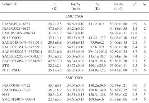
Table 1.Target information for the Magellanic YSO sample analysed using Herschel spectroscopy. References for the information in the source properties column are as follows: 1:Oliveira et al.(2013); 2:Breen et al.(2013); 3:Ward et al.(2017); 4:Oliveira et al.(2009); 5:

Seale et al.(2009); 6:Seale et al.(2011); 7:Imai et al.(2013) and references therein for a compilation of H2O maser sources in the LMC; 8:

Green et al.(2008) for a compilation of OH and CH3OH masers in the LMC; 9:Ward et al.(2016) and references therein for a recent review

of the N 113 region; 10: probable YSO detected with Herschel (Seale et al. 2014) but not detected with Spitzer; 11:Shimonishi et al.(2010). Radio detections for SMC YSOs are fromOliveira et al.(2013, and references therein); archival images (Hughes et al. 2007;Bozzetto et al. 2017) were inspected to identify radio counterparts of the LMC YSOs. Sources # 7A and 7B are not resolved in the PACS observations but a separate PACS spectrum was extracted for # 7C; these three sources are unresolved at SPIRE wavelengths. This results in 20 sources resolved across the full Herschel (PACS and SPIRE) wavelength range, but PACS spectra were extracted for 21 sources. The last column indicates which PACS spectral ranges from Table2are not observed for each object; all sources are observed with the SPIRE FTS except for #11 (N 113 YSO-4, see also top panel in Fig.1); a further four sources (#3, 8, 9 and 16) have been observed with SPIRE FTS but the signal-to-noise ratio for the line emission is too low for a reliable analysis (Sect.7).

# Source ID RA (J2000) Dec Source properties Ref. Lines not observed

(h:m:s) (◦_:′_:′′_{) or with low SNR}

SMC YSOs

1 IRAS 00430−7326 00:44:56.3 −73:10:11.6 ice; H2O maser; UCH ii; radio 1,2,3 OH 84 µm

2 IRAS 00464−7322 00:46:24.5 −73:22:07.3 ice 1 OH 84 µm, [O iii], H2O 108 µm, CO 186 µm

3 S3MC 00541−7319 00:54:03.6 −73:19:38.4 ice 1 low SNR SPIRE FTS

4 N 81 01:09:12.7 −73:11:38.4 protocluster; UCH ii; radio 3 OH 79 µm

5 SMC 012407−73090 (N 88A) 01:24:07.9 −73:09:04.1 protocluster; UCH ii 3 LMC YSOs

6 IRAS 04514−6931 04:51:11.4 −69:26:46.7 ice; radio 4 OH 79 µm

7A SAGE 045400.2−691155.4 04:54:00.1 −69:11:55.5 ice; H2O maser 5,6,7

7B SAGE 045400.9−691151.6 04:54:00.9 −69:11:51.6 ice 5

7C SAGE 045403.0−691139.7 04:54:03.0 −69:11:39.7 ice 5,6

8 IRAS 05011−6815 05:01:01.8 −68:10:28.2 H2O, OH, CH3OH masers 7,8 low SNR SPIRE FTS

9 SAGE 051024.1−701406.5 05:10:24.1 −70:14:06.5 ice 5,6 low SNR SPIRE FTS

10 N 113 YSO-1 05:13:17.7 −69:22:25.0 H2Omaser; radio 7,8,9

11 N 113 YSO-4 05:13:21.4 −69:22:41.5 H2O maser?; protocluster; UCH ii; radio 7,9 SPIRE FTS

12 N 113 YSO-3 05:13:25.1 −69:22:45.1 H2O, OH masers; protocluster; UCH ii; radio 7,8,9

13 SAGE 051351.5−672721.9 05:13:51.5 −67:27:21.9 ice; radio 5,6 OH 79 µm

14 SAGE 052202.7−674702.1 05:22:02.7 −67:47:02.1 ice; radio 5,6

15 SAGE 052212.6−675832.4 05:22:12.6 −67:58:32.4 ice; radio 5,6

16 SAGE 052350.0−675719.6 05:23:50.0 −67:57:19.6 ice; radio 5,6 low SNR SPIRE FTS

17 SAGE 053054.2−683428.3 05:30:54.2 −68:34:28.3 ice; radio 5,6 OH 79 µm

18 IRAS 05328−6827 05:32:38.6 −68:25:22.6 ice; radio 4

19 LMC 053705−694741 05:37:05.0 −69:47:41.0 HerschelYSO; radio 10 OH 79 µm

20 ST 01 05:39:31.2 −70:12:16.8 ice; radio 11

IRAS 00430−7326 and IRAS 00464−7322 exhibit extended out-flow morphologies in H21−0S(1) at 2.1218 µm; IRAS 00430−7326

(a H2O maser source,Breen et al. 2013) is particularly suggestive

of a wide, relatively uncollimated outflow that is bound by the pres-ence of a disc detected in CO bandhead emission (the first such de-tection in any extragalactic YSO). By contrast S3MC 00541−7319 is a compact emission line source.Ward et al.(2017) also analysed two well-known regions, N 81 and SMC 012407−73090 (N 88A). Both IR sources are in fact resolved into protoclusters. N 81 in-cludes a source that exhibits resolved bipolar H2 emission, while

N 88A is dominated by an expanding bubble of ionised gas (seen in Brγ emission) surrounded by a very conspicuous H2emission arc.

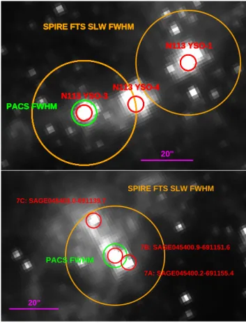
The sample includes YSOs in N 113, one of the most promi-nent star forming regions in the LMC.Sewiło et al.(2010) pro-vided a compilation of the indicators for ongoing star formation in the region (see their Fig. 2) that we summarise here. A dense dust lane seems to be heated and/or compressed by prominent Hα emis-sion bubbles (e.g.,Oliveira et al. 2006), seen also in the Magellanic Cloud Emission Line Survey (MCELS1_{) Hα, [O iii] and [S ii]}

im-ages. N 113 also hosts the largest number of H2O and OH masers

and the brightest H2O maser in the LMC (e.g.,Green et al. 2008;

Ellingsen et al. 2011). Figure1(top) shows the three conspicuous YSO sources in this region; N 113 YSO-1 and N 113 YSO-4 are at distances of ∼ 45′′ _{and 20}′′ _{respectively from N 113 YSO-3}2_. These three massive YSOs were analysed by Ward et al.(2016) using SINFONI/VLT (see above). They found that even though the Spitzer IRS spectra of the sources are similar (dominated by polycyclic aromatic hydrocarbon (PAH) and forbidden line emis-sion), the nature of the three sources are in fact quite different. N 113 YSO-1 is a single relatively quiescent and compact source, while N 113 YSO-3 is a protocluster dominated by an expanding ultra-compact Hii region (UCHii) accompanied by another more compact YSO and a bright H2source (suggestive of a YSO with an

outflow), all within a 3′′

FOV. N 113 YSO-4 is in turn resolved into

1 _{UM/CTIO MCELS Project/NOAO/AURA/NSF}

2 _{Sewiło et al. (2010) labelled N 113 YSO-1, while N 113 YSO-3 and}

N 113 YSO-4 were identified inWard et al.(2016); N 113 YSO-2 is located further away to the North (Sewiło et al. 2010).

SPIRE FTS SLW FWHM PACS FWHM N113 YSO-1 N113 YSO-4 N113 YSO-3 SPIRE FTS SLW FWHM PACS FWHM N113 YSO-1 N113 YSO-4 N113 YSO-3 SPIRE FTS SLW FWHM PACS FWHM N113 YSO-1 N113 YSO-4 N113 YSO-3 20" SPIRE FTS SLW FWHM PACS FWHM N113 YSO-1 N113 YSO-4 N113 YSO-3 20" SPIRE FTS SLW FWHM PACS FWHM 7C: SAGE045403.0-691139.7 7A: SAGE045400.2-691155.4 7B: SAGE045400.9-691151.6

Figure 1. Spitzer 3.6 µm image of N 113 (top) and SAGE 045400.9−691151.6 (bottom), identifying the YSO sources (red circles). Also indicated is the PACS beam full-width-at-half-maximum (green circle, FW H M = 9.′′5 at the wavelength of the [O i] 63 µm and [O iii] 88 µm lines, Altieri & Vavrek 2013), and the nominal SPIRE FTS beam (orange circle, FW H M = 40′′_{for SLW,Valtchanov 2017). Note that}

the FW H M for the [C ii] beam is ∼ 20% larger. North is to the top and East is to the left.

two continuum sources, one expanding UCHii and a more com-pact source. The complexity of this region is undeniable, and the origin of the observed maser emission remains unclear. Using data obtained with the Atacama Large Millimeter/Submillimeter Array (ALMA),Sewiło et al.(2018) reported on the first extragalactic de-tection of several complex organic molecules in two hot cores in the neighbourhood of N 113 YSO-1 and YSO-3.

Figure1 shows the Herschel pointings with multiple YSO sources: the N 113 region described above (top) and SAGE 045400.9−691151.6 and its neighbours (bottom; #7 in Ta-ble1). While resolved in the Spitzer IRAC bands, #7A and 7B are not resolved beyond 24 µm (their separation is approximately 6′′

); both sources are strong ice sources (Seale et al. 2009,2011) and are associated with a H2O maser (Imai et al. 2013). Another nearby

source (#7C, separation ∼ 20′′

) is a weak ice source (Seale et al. 2009,2011). These three sources are unresolved at Herschel SPIRE wavelengths; #7A & 7B are unresolved in the PACS spectra, but a PACS spectrum for #7C could be extracted from the observations (Sect.3.1). Other sources visible in Fig.1(bottom) are relatively blue, for instance they are not detected in the PACS 100 µm im-ages. Henceforth we will refer to unresolved sources #7A & 7B collectively as SAGE 045400.9−691151.6. All other pointings are relatively simple point sources at this resolution.

Table 2.Transitions observed with the PACS spectrometer (line spectroscopy mode). As described in the text, 19 pointings trans-late to 21 YSO sources resolved with PACS; the last column tallies how many sources are observed for each spectral region (see also Table1).

Species Transition Rest λ(µm) N

[O i] 3_P 0–3P2 63.18 21 OH 2_Π 1/2(J = 1/2) –2Π3/2(J = 3/2) 79.11, 79.18 19 OH 2Π3/2(J = 7/2 – J = 5/2) 84.4, 84.6 16 [O iii] 3P1–3P0 88.36 20 o-H2O 212– 101 179.52 21 [C ii] 2P3/2–2P1/2 157.74 21 o-H2O 221– 110 108.07 20 CO 14 – 13 185.99 20

3 HERSCHEL OBSERVATIONS AND DATA REDUCTION The observations discussed here were obtained as part of two Her-schelOpen Time programmes. These two programmes (proposal identifications OT1_joliveir_1 and OT2_joliveir_2) amounted to 73.4 h of Herschel observing time.

3.1 PACS spectra

All the targets in Table1were observed using the PACS spectrom-eter: an integral field unit made of 5 × 5 square spaxels – total FOV ∼47′′_×

47′′

) – operating in the 50 − 200 µm range. Selected wave-length ranges were targeted to obtain spectra that include molecu-lar and atomic lines of interest (Table2). All wavelengths quoted throughout this paper are rest wavelengths in vacuum. The spec-tral resolution varies between λ/∆λ ∼ 3000 (for [O i] at 83 µm) and ∼1000 (for H2O at 108 µm).

The targets are unresolved in all Spitzer and Herschel images, and thus single-pointing mode was used. The emission from the ISM surrounding the targets precluded the use of the chop/nod mode, and instead we observed all targets in unchopped line scan mode, selecting patches of sky with negligible 160 µm emission for the offset measurement (dominated by the emission from the telescope). For this observing mode the continuum level can be re-covered in a reliable way only for bright sources (Altieri & Vavrek 2013); many of our targets are relatively faint in all or some of the observed spectral ranges, therefore continuum uncertainties of at least ∼30% are expected. However, both the line profiles and strength are reliably recovered in this observing mode. The number of objects targeted for each PACS range is detailed in the last col-umn of Table2; ranges not observed for each target are listed in the last column of Table1.

Spectra were reduced as advised within the Herschel Inter-active Processing Environment (HIPE3_{, v.10.0.2, PACS calibration} tree version 48) using standard recipes for this type of observations. Reduced observations were retrieved from the database but spectral flatfielding was performed independently step-by-step: this is a cru-cial task for improving the signal-to-noise ratio (SNR) of the final spectra, and it is advised to monitor the task’s progress closely. For

3 _{HerschelInteractive Processing Environment HIPE is a joint development}

by the Herschel Science Ground Segment Consortium, consisting of ESA, the NASA Herschel Science Center, and the HIFI, PACS, and SPIRE con-sortia.

more information, the reader should refer to the “PACS Data Re-duction Guide: Spectroscopy”4_{. The spectra were checked against} subsequent database, software and calibration releases; no further improvements in the quality of the spectra were forthcoming.

For most pointings the intended target is located in the central spaxel. The spectrum for the central spaxel (2,2) was extracted from the rebinned data cubes (slicedFinalCubes) and a point source flux loss correction was applied (no correction for slight pointing offsets and pointing jitter can be applied to unchopped observations due to the uncertainties in the continuum level). Line flux measure-ments for the lines of interest (Table2) were performed on these extracted spectra, using standard spectral fitting tools within HIPE. All lines are spectrally unresolved. Line fluxes for all lines detected with PACS are listed in TableD1; example spectra are shown in Fig.C1.

Referring to Table1, sources SAGE 045400.2−691155.4 and SAGE 045400.9−691151.6 (#7A and 7B) are blended as observed with the PACS spectrometer (the observations are actually cen-tred on #7B); these two sources fall on the central spaxel (2,2) while SAGE 045403.0−691139.7 (#7C) falls on spaxel (1,3). N 113 YSO-4 was not directly targeted with a separate PACS observation, but it falls onto the FOV of the observations for both N 113 YSO-1 and N 113 YSO-3; this source is however better centred for the ob-servation of N 113 YSO-3, falling on spaxel (4,3). Spectra for those secondary sources are extracted from the spaxels mentioned and the point source flux loss correction is applied; centring on spaxels other than the central one is obviously not optimal, therefore for those sources there are additional flux losses that cannot be cor-rected for. To summarise, the sample comprises 19 PACS point-ings that result in 21 sources for which spectra were extracted. The analysis of all lines detected in the PACS range is described in Sec-tion6.

For some sources, [O i], [C ii] and [O iii] line emission is de-tected in spaxels other than the central spaxel (see Sect.6.1.1), i.e. a point source is superposed on an extended environmental contri-bution. In order to analyse the morphology of the emission region and to estimate the environmental contribution to the on-source line emission, we measured the emission line flux for these lines across all spaxels. Since rebinned data cubes do not have a regular sky footprint (they are organised spatially as a slightly irregular 5 × 5 grid of 25 spaxels), we projected the data from the irregular native sky footprint onto a regular 3′′

sky grid, producing line flux maps (we made use of final data product scripts available within HIPE). Such maps should not be used for science measurements but are ad-equate to estimate the contribution of the off-source emission. More detail on how these flux maps are used is given in Sect.6.1.1. When detected, H2O, OH and CO emission is present only in the central

spaxel; compact OH absorption is detected for a small number of sources (see Section6.2).

3.2 SPIRE FTS spectra

We observed our YSO targets using the SPIRE FTS in single-pointing mode with sparse image sampling to obtain spectra from 447 to 1546 GHz (∼ 190 − 650 µm) with spectral resolution ∆ν =1.2 GHz, covering the CO ladder from transitions12_{CO (4−3)}

to (13−12) (Table3). The full wavelength coverage was achieved by using two bolometer arrays (SPIRE Short/Long Wavelength, re-spectively SSW and SLW) providing a nominal 2′_{unvigneted FOV.}

4 _{http://herschel.esac.esa.int/hcss-doc-10.0/}

Table 3.Transitions in the SPIRE FTS range.

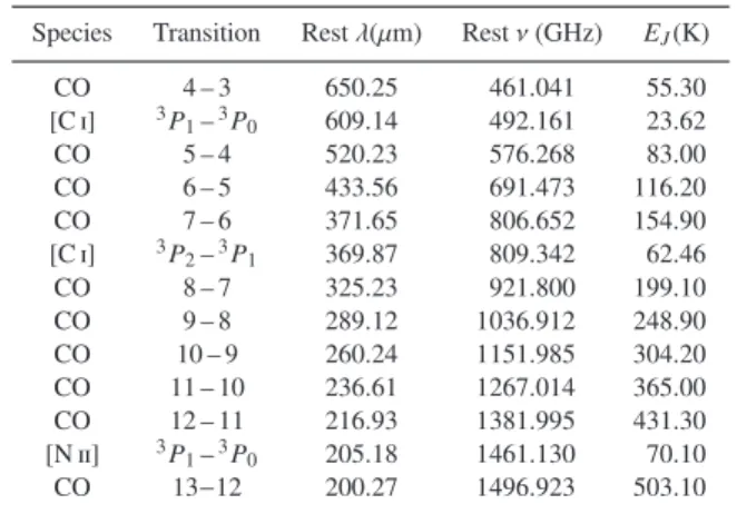
Species Transition Rest λ(µm) Rest ν (GHz) EJ(K)

CO 4 – 3 650.25 461.041 55.30 [C i] 3_P 1–3P0 609.14 492.161 23.62 CO 5 – 4 520.23 576.268 83.00 CO 6 – 5 433.56 691.473 116.20 CO 7 – 6 371.65 806.652 154.90 [C i] 3_P 2–3P1 369.87 809.342 62.46 CO 8 – 7 325.23 921.800 199.10 CO 9 – 8 289.12 1036.912 248.90 CO 10 – 9 260.24 1151.985 304.20 CO 11 – 10 236.61 1267.014 365.00 CO 12 – 11 216.93 1381.995 431.30 [N ii] 3_P 1–3P0 205.18 1461.130 70.10 CO 13−12 200.27 1496.923 503.10

In total 19 SPIRE FTS pointings were performed. No SPIRE FTS spectrum is available for N 113 YSO-4; even though it falls within the FOV of the observations of both YSO-1 and YSO-3 (Fig.1), the positions of the individual SSW and SLW bolometers do not allow for a spectrum to be extracted (see below). Referring to Table1, a single spectrum was extracted that includes the contributions of sources #7A, 7B and 7C (see also bottom panel in Fig.1).

FTS spectra were reduced as advised within HIPE3 _(v.10.0.1, SPIRE calibration tree spire_cal_11_0) using standard recipes for this type of observations (“SPIRE Data Reduction Guide: Spec-troscopy”5_{, see alsoFulton et al. 2016). Background subtraction} was performed using dedicated HIPE scripts; we found that using carefully selected off-axis detectors for the subtraction provided the best results (in terms of spectral shape and agreement between the SSW and SLW bands), compared to using dark sky observations from the same operational day (this is expected for relatively faint sources). The data products were checked against subsequent re-processings with more advanced HIPE and SPIRE calibration ver-sions for representative sources; no significant improvements were found. Finally the FTS spectra of the targets were extracted from the SLWC3 and SSWD4 detectors. Note that given the nature of the observations (single pointing sparse map), SSW and SLW detector alignment is only achieved for the intended source; thus we cannot extract fully calibrated spectra for other sources in the FOV (e.g., N 113 YSO-4).

The majority of SPIRE FTS spectra show a discontinuity be-tween the SSW and SLW bands. For most sources the disconti-nuity is such that the SSW flux drops below the SLW flux in the overlap region. This results from the fact that the SLW beam di-ameter is approximately a factor of 2 larger than that of SSW and it affects any sources that are semi-extended at these wavelengths. For such sources the final spectra are corrected to an equivalent beam size (a Gaussian beam of 40′′

) using the Semi-extended Correction Tool(SECT, for more details see the “SPIRE Data Reduction Guide: Spectroscopy” already mentioned). It should be noted that there is an implicit assumption that the spatial extension of the continuum and line emitting regions is the same. In total 15 sources out of 19 had a SECT correction applied.

For remaining four sources the discontinuity is reversed, i.e. the SLW flux drops below the SSW flux. This is a calibration effect due to rapidly changing detector temperatures after the cooler was

recycled; it affects observations taken at the beginning of an FTS observing block, as is the case for the four sources in question. Specialists at the Herschel Helpdesk reprocessed and corrected the FTS spectra affected.

Line emission intensities were obtained by fitting the un-apodised spectra with a low-order polynomial combined with a sinc profile for each line of interest (Table3), using standard spectral fitting tools within HIPE. Line fluxes for all lines and transitions detected with SPIRE FTS are listed in TableD2; example spectra are shown in Fig.C1. A full characterisation of the SPIRE FTS performance can be found inHopwood et al.(2015, and references therein), including discussions of line flux and velocity measure-ments and performance (see also Section7.1). For four of the 19 SPIRE FTS pointings the SNR for the CO line fluxes (TableD2) is deemed too low for a meaningful analysis (see also Table1); for these sources we compute total CO luminosities only, and no fur-ther analysis is performed. The analysis of emission lines in the SPIRE range (i.e. CO, [N ii] and [C i]) is described in Section7.

4 FAR-IR LUMINOSITY AND DUST TEMPERATURE Even though the Magellanic sample was selected trying to avoid sources with a complex background, this was not always the case. We have also found that the Spitzer IRAC and MIPS Magellanic photometric catalogues (Meixner et al. 2006;Gordon et al. 2011) are not always reliable or complete for massive Magellanic YSOs. Such sources are often marginally extended to the extent that they are absent from those point source catalogues (see discussion in

Sewiło et al. 2013). Furthermore, massive YSO fluxes at 70 µm of-ten seem anomalously high compared to for instance PACS fluxes. Since aperture photometry has been shown to perform better for samples such as ours (Gruendl & Chu 2009;Sewiło et al. 2013), we instead performed aperture photometry tailoring the parameters to each source environment. The measured fluxes are presented in TableA1. They are used to estimate the integrated IR luminosity for each target.

Sewiło et al.(2010) described the difficulties of using Spitzer-optimised YSO spectral energy distribution (SED) fitters (e.g.,

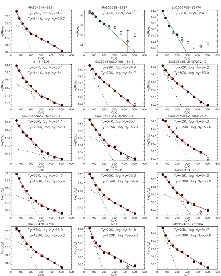
Robitaille et al. 2006) to fit simultaneous Spitzer and Herschel pho-tometry: the model components do not fully account for the en-velope of cooler dust and gas further away from the source that emits little at shorter wavelengths but contributes significantly in the Herschel bands. For the line emission analysis presented in this work, it is crucial to constrain the cold dust emission that is the spatial counterpart to the emission lines measured with PACS and SPIRE. The spatial resolution of the observations across the avail-able wavelength range (3.6 − 500 µm) is also very disparate. Im-proved SED models are available (Robitaille 2017) but limitations remain; namely only Galactic dust emission without the contribu-tion of PAH emission is included, and a single source of emission is assumed. Since for our analysis we simply require an estimate of the dust temperature and total integrated far-IR emission, we opt instead for the simpler approach of fitting a two temperature component modified blackbody function to the available photome-try. A cold blackbody component is responsible for the majority of the far-IR emission (details below), however a hotter component is needed to fit the Spitzer photometry at 24 µm.

To fit the two component modified blackbody we use the blackbody python code, available as part of the agpy

collec-tion of astronomical software6_{. It uses a Markov-chain Monte} Carlo (MCMC) Bayesian statistical analysis to constrain the mod-ified blackbodies’ temperatures and fluxes; we use an emissiv-ity spectral index β = 1.5 (see alsoSeale et al. 2014). We adopt gas-to-dust ratios of 400 and 1000 (e.g., Roman-Duval et al. 2014), and distances of 50 kpc and 60 kpc (e.g.,Schaefer 2008;

Hilditch, Howarth & Harries 2005), respectively for the LMC and SMC. For further details on the modified blackbody expression and adopted dust opacity κνrefer toBattersby et al.(2011). Examples

of the two component modified blackbody fits are shown in Fig.B1. Integrated total IR luminosity and cold dust temperature are listed in Table4; L(> 30 µm) accounts for the majority of the contribution of the cold dust blackbody, while L(> 10 µm) includes the contribution of the warm blackbody; the ratio L(> 30µm)/L(> 10 µm) ranges between 67% and 93% (median 77%). Cold dust temperatures vary between 22 and 39 K (median 31.6 K); the temperature of the warmer blackbody is not well con-strained. L(> 10 µm) varies between ∼ (5 − 32) ×103_L

⊙ (median

∼6.3 ×103_L

⊙). For the same integrated luminosity there is a

ten-dency for SMC sources to have higher blackbody temperatures, re-flecting higher dust temperature (see alsovan Loon et al. 2010a,b).

Seale et al.(2014) determined temperatures and far-IR luminosi-ties for a subset of our sources, using Herschel photometry only. In general the temperatures agree within the uncertainties, but in some cases our derived temperatures are higher given that we took into account additional photometry (70 µm MIPS fluxes are crucial in constraining the dust temperature). The integrated far-IR lumi-nosities fromSeale et al.(2014) are in good agreement with our L(> 70 µm) fluxes (not tabulated). In the subsequent discussions we adopt L(> 10 µm) as the object’s total IR luminosity LTIR. For these

type of objects LTIRdoes not differ significantly from the

bolomet-ric luminosity Lbol.

5 GALACTIC MASSIVE YSO COMPARISON SAMPLE One of the challenges in observing and interpreting the data of massive YSOs in the Magellanic Clouds lies with the fact that observations probe different spatial scales compared to Galactic massive YSOs. A sample of high luminosity Galactic YSOs was observed with Herschel (Karska et al. 2014), however the spatial scales probed (corresponding to the central PACS spaxel only) sam-ple very different spatial components in the massive YSO environ-ment compared to the Magellanic Herschel observations. Further-more, the [C ii] emission is often saturated for those sources. With this in mind, we instead compiled a Galactic comparison sample of massive YSOs observed with the Infrared Space Observatory (ISO,Kessler et al. 1996). In fact, the region sampled by PACS at 156 µm at a distance of the LMC (∼ 50 kpc) is equivalent to the region sampled by the ISO Long-Wavelength Spectrograph (ISO LWS,Clegg et al. 1996) at a distance of ∼ 8 kpc (ISO-LWS equiv-alent beam size information fromGry et al. 2003).

We identified 22 massive YSOs observed with ISO LWS with luminosities in the range ∼ (5−500) ×103_L

⊙ and located at

dis-tances in the range ∼ 1−10 kpc (see TableE1for individual ob-ject information); the spectra of these sources were retrieved from the ISO Data Archive7_{(IDA). Of these 22 spectra we selected 19}

6 _{agpy is authored by Adam Ginsburg and is available at}

https://github.com/keflavich/agpy.

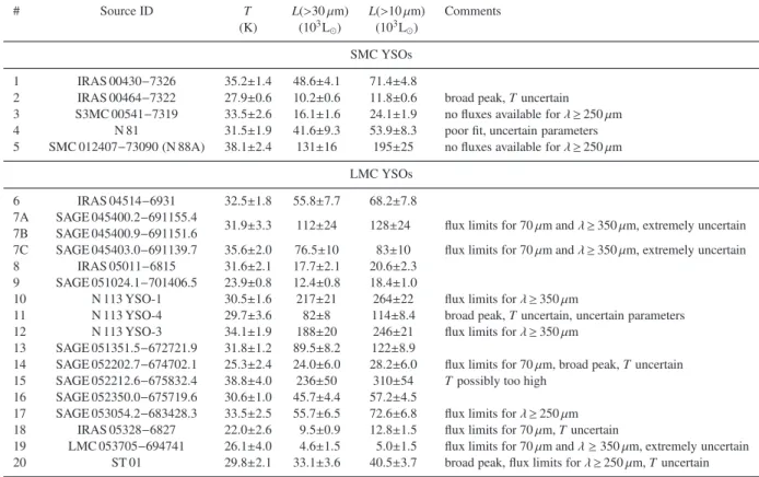
Table 4.Parameters for the modified blackbody fits to the available photometry (see Table A1). The emissivity spectral index is β = 1.5. Inte-grated luminosities are tabulated for wavelengths longer than 10 µm and 30 µm, L(>10 µm) and L(>30 µm) respectively. The temperature of the hotter modified blackbody that contributes to L(>10 µm) (see text) is poorly constrained (typically T ∼ 100 K). The comments column in-dicates missing fluxes and provides an empirical assessment of the reliability of the fitted parameters. For LMC053705−694741 the tabulated parameters are particularly uncertain: there are two bright sources within ∼ 25′′

, and the fit is rather conservative meaning the luminosities could easily be higher by a factor 2. L(>10 µm) is adopted as LTIRfor all subsequent discussions.

# Source ID T L(>30 µm) L(>10 µm) Comments

(K) (103L⊙) (103L⊙)

SMC YSOs 1 IRAS 00430−7326 35.2±1.4 48.6±4.1 71.4±4.8

2 IRAS 00464−7322 27.9±0.6 10.2±0.6 11.8±0.6 broad peak, T uncertain 3 S3MC 00541−7319 33.5±2.6 16.1±1.6 24.1±1.9 no fluxes available for λ ≥ 250 µm 4 N 81 31.5±1.9 41.6±9.3 53.9±8.3 poor fit, uncertain parameters 5 SMC 012407−73090 (N 88A) 38.1±2.4 131±16 195±25 no fluxes available for λ ≥ 250 µm

LMC YSOs 6 IRAS 04514−6931 32.5±1.8 55.8±7.7 68.2±7.8 7A SAGE 045400.2−691155.4

31.9±3.3 112±24 128±24 flux limits for 70 µm and λ ≥ 350 µm, extremely uncertain 7B SAGE 045400.9−691151.6

7C SAGE 045403.0−691139.7 35.6±2.0 76.5±10 83±10 flux limits for 70 µm and λ ≥ 350 µm, extremely uncertain 8 IRAS 05011−6815 31.6±2.1 17.7±2.1 20.6±2.3

9 SAGE 051024.1−701406.5 23.9±0.8 12.4±0.8 18.4±1.0

10 N 113 YSO-1 30.5±1.6 217±21 264±22 flux limits for λ ≥ 350 µm

11 N 113 YSO-4 29.7±3.6 82±8 114±8.4 broad peak, T uncertain, uncertain parameters 12 N 113 YSO-3 34.1±1.9 188±20 246±21 flux limits for λ ≥ 350 µm

13 SAGE 051351.5−672721.9 31.8±1.2 89.5±8.2 122±8.9

14 SAGE 052202.7−674702.1 25.3±2.4 24.0±6.0 28.2±6.0 flux limits for 70 µm, broad peak, T uncertain 15 SAGE 052212.6−675832.4 38.8±4.0 236±50 310±54 Tpossibly too high

16 SAGE 052350.0−675719.6 30.6±1.0 45.7±4.4 57.2±4.5

17 SAGE 053054.2−683428.3 33.5±2.5 55.7±6.5 72.6±6.8 flux limits for λ ≥ 250 µm 18 IRAS 05328−6827 22.0±2.6 9.5±0.9 12.8±1.5 flux limits for 70 µm, T uncertain

19 LMC 053705−694741 26.1±4.0 4.6±1.5 5.0±1.5 flux limits for 70 µm and λ ≥ 350 µm, extremely uncertain 20 ST 01 29.8±2.1 33.1±3.6 40.5±3.7 broad peak, flux limits for λ ≥ 250 µm, T uncertain

for which both the [O i] and [C ii] lines are in emission. The rel-atively low SNR of the spectra, especially at shorter wavelengths, implies we were only able to measure fluxes for the strongest emis-sion lines: [C ii] at 158 µm, [O i] at 63 and 145 µm, [O iii] at 88 µm, [N ii] at 122 µm and CO at 186 µm. To ensure uniformity in the way fluxes are estimated, we measured all line fluxes from archival spectra rather than using published measurements. More details on this massive YSO comparison sample are provided in AppendixE. The Magellanic and Galactic sample properties are further dis-cussed in Sect.8.2.2.

6 RESULTS: PACS SPECTRA 6.1 [C ii], [O i] and [O iii] emission 6.1.1 Emission line morphology

[C ii], [O i] and [O iii] emission is often detected beyond the central spaxel. [C ii] emission is usually present across the FOV, covering it completely for all but two sources. [O i] emission completely cov-ers the FOV in 11 out of 19 pointings, and is present beyond the central spaxel in eight others. Crucially there is always a flux en-hancement in the central spaxel related to the point source targeted, i.e. the point source contribution is superposed on extended diffuse environmental emission.

We investigate the morphology of the extended emission lines

observed, making use of the line emission maps described in Sect.3.1. Taking into account the beam size for each line, these maps are used to estimate the environmental contribution as a frac-tion of the peak flux at the source posifrac-tion; that contribufrac-tion is subtracted from the measured line flux for the source, and a point source correction is applied (Sect.3.1). For [O i] the environmen-tal emission accounts for typically 20% (maximum 70%) in the LMC and 7% (maximum 11%) in the SMC; for [C ii] it accounts for typically 42% (maximum 85%) in the LMC and 30% (maxi-mum 50%) in the SMC. Clearly the extended diffuse contribution is more important for [C ii] emission than for [O i] emission (see also

Lebouteiller et al. 2012), but it is also more significant for LMC sources compared to SMC sources. Furthermore, the morphology of the [C ii] and [O i] extended emission follows the dust emission (e.g., 100 µm PACS emission), even if the [O i] emission is gener-ally less extended (Fig.2).

The [O iii] emission line morphology is as expected some-what different, given its distinct physical origin (see discussion in next section). Out of the 18 observations in this spectral range (IRAS00464−7322 was not observed), six sources are not detected in [O iii] line emission and four sources exhibit compact emission at the central spaxel only. For the other eight pointings, emission extends across the FOV: for two of these the intended target (that falls on the central spaxel) is the source of the strongest emission; we discuss below the remaining six pointings in more detail.

[OI] [OIII] [CII] N 113 20 arcsec SAGE052212.6-675832.4 20 arcsec SAGE051351.5-672721.9 20 arcsec SAGE04500.9-691151.6 20 arcsec YSO−1 YSO−4 YSO−3 S04503.0−691139.7 S04500.2−691155.4 S04500.9−691151.6

Figure 2. Line emission maps for [C ii] (red), [O iii] (green) and [O i] (blue). The YSOs in N 113, SAGE 052212.6−675832.4, SAGE 045400.9−691151.6 and SAGE 051351.5−672721.9 (clockwise from top left) are shown (black circles with diameter 9.′′

5, the FW H M of the [O i] and [O iii] beams). North is to the top and East to the left in all maps.

N 113, YSO-1 and YSO-4 are strong [O iii] emission line sources, while YSO-3 is actually consistent with environmental emission or contamination from YSO-4 (the strongest [O iii] emitter in this region). Strong emission also originates from locations at the FOV’s northern and western edges. For four other pointings the peak [O iii] emission is displaced from the central spaxel. Fig-ure2 (bottom right) shows the line emission in the region of SAGE 045400.9−691151.6. While the spatial distributions of [O i] and [C ii] emission are similar (tracing the dust emission), the [O iii] emission is clearly offset. This morphology is very suggestive of a large ionised gas bubble (as seen also in MCELS images) with the three YSOs embedded in the dust at its rim. The observed emis-sion for SAGE 045400.9−691151.6 and N 113 above are reminis-cent of the emission line maps of LMC-N 11, in which the spatial distribution of [O iii] emission seems anti-correlated to that of [C ii] (Lebouteiller et al. 2012).

Two other sources with off-source [O iii] peak emission are also shown in Fig.2: SAGE 051351.5−672721.9 (bottom

left) and SAGE 052212.6−675832.4 (top right) are also de-tected in the MCELS [O iii] map. While there might be a slight problem with source centring on the spaxel, it is nev-ertheless very clear that the [O iii] emission is not point-source like. Instead it originates from the immediate surround-ing H ii regions: SAGE 051351.5−672721.9 is situated ∼20′′

from the ionising B[e] supergiant Hen S22 (Chu et al. 2003), while SAGE 052212.6−675832.4 is just ∼10′′ _{away from an}

O7V star within N 44C (Chen et al. 2009). Therefore we con-clude that the observed emission for SAGE 051351.5−672721.9 and SAGE 052212.6−675832.4, as well as N 113 YSO-3 and SAGE 045400.9−691151.6 above, is likely mostly ambient.

A final source, SAGE 053054.2−683428.3 (not shown in Fig.2), exhibits compact [O iii] emission centred on spaxel (2,3) su-perposed on more extended environmental emission. Inspection of the emission line centroids for several spaxels reveals wavelength shifts that are a tell-tale sign that the source is not well centred in the central spaxel and is offset in the dispersion direction (i.e. from

spaxel (2,2) to spaxel (2,3), for more details refer toVandenbussche 2011). Thus, the observed compact [O iii] emission is very likely associated with the source on the central spaxel but it is affected by poor source centring.

In brief, [O iii] emission associated with the YSO targets is detected for a total of nine sources, six in the LMC and three in the SMC.

6.1.2 Emission line diagnostics and correlations

In this section we compare line emission for [C ii], [O i] and [O iii] for the Magellanic sample and the Galactic ISO sample. Emission lines like [O i] and [C ii] are often used to diagnose the environmental conditions of massive YSOs, since they are amongst the main contributors to line cooling. The difficulty is that such lines can originate from distinct components within the star formation environment. In particular in their later evolution-ary stages, massive YSOs are copious producers of ultraviolet pho-tons; as a result they often exhibit expanding compact H ii re-gions, even while still actively accreting from their envelopes (e.g.,

Beuther et al. 2007). These emerging H ii regions help shape the structure and chemistry of the YSO environment. In schematic terms (seeKaufman, Wolfire & Hollenbach 2006, for an actual di-agram and further details), two main regions can be distinguished: the H ii region itself marks the sphere of influence of H-ionising photons (hν ≥ 13.6 eV); less energetic far-untraviolet (FUV) pho-tons (6 eV ≤ hν ≤ 13.6 eV) penetrate into the adjacent neutral and molecular hydrogen gas and play a significant role in the chem-istry, heating and ionisation balance of these photodissociation re-gions (e.g.,Tielens & Hollenbach 1985). PDRs include both the neutral dense gas near the YSOs but also the neutral diffuse ISM. Energetic outflows are also a ubiquitous phenomenon in mas-sive star formation, driving shocks through the surrounding gas (e.g., Beuther et al. 2007; Bally 2016). Both PDRs and shocks contribute to the excitation of far-IR [O i], [C ii] and CO emis-sion (e.g.,Hollenbach & McKee 1989;Kaufman et al. 1999,2006), while shocks are particularly important to H2O and OH excitation

(e.g.,van Dishoeck et al. 2011;Wampfler et al. 2013).

The ionisation potential for neutral carbon C0_{is just 11.26 eV,}

therefore [C ii] emission can originate not only in H ii regions, but also in PDRs and diffuse atomic and ionised gas (e.g.,

Kaufman et al. 1999, 2006). On the other hand, [O i] is only found in neutral gas (the ionisation potential for O0 _{is 13.62 eV,}

just above that for hydrogen), and emission arises from warm, dense regions. [O i] emission can originate from deeper inside the PDR than [C ii] since some atomic oxygen remains in re-gions where all carbon is locked into CO. [O i] emission also originates from shocks in molecular outflows that can contribute in a small fraction to [C ii] emission (resulting in [O i]/[C ii] flux ratios of >∼ 10, Hollenbach & McKee 1989). Given the relatively high ionisation potential for O+

(35 eV), [O iii] emission originates from H ii regions, rather than the diffuse interclump medium (e.g.,

Cormier et al. 2015, for a thorough description of these line proper-ties). We note that the ionised gas emitting [O iii] emits little [C ii] (the ionisation potential for C+_{is 24.38 eV); ionised [C ii]-emitting}

gas is traced instead by [N ii] emission (the ionisation potential for N0_{is 14.53 eV).}

It is important to quantify the contribution of ionised gas to [C ii] emission, before comparing [C ii] and [O i] line fluxes. Con-sidering an integrated PDR and H ii region model,Kaufman et al.

(2006) find that for solar metallicity [C ii] emission is always dom-inated by the PDR contribution as opposed to the contribution of

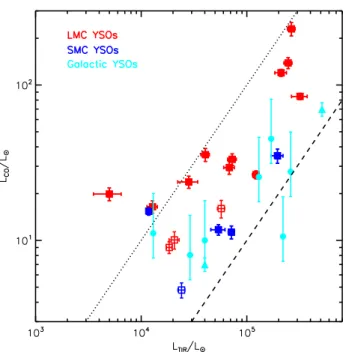
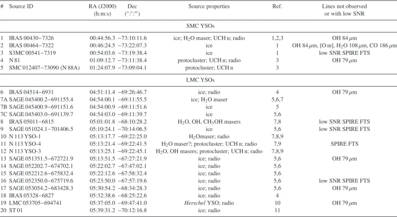
Figure 3. FIR line correlations: [C ii] versus [O i] luminosities (top panel), [C ii] luminosity versus LTIRluminosity (middle) and [O iii] versus [O i]

lu-minosities (bottom). Squares represent Magellanic YSOs (respectively red and blue for the LMC and the SMC) and circles represent Galactic YSOs. Line luminosities for both samples have been corrected for the ionised gas contribution to [C ii] emission (for sources with [N ii] emission (yellow sym-bols), see text). Only the Magellanic sample has been corrected for contribu-tion of the extended diffuse emission (see text for details); the colour-coded lines indicate the size of this correction.

the ionised gas in the H ii region; furthermore the H ii region contri-bution increases for higher metallicity environments. As described in Sect.7.5.1, we estimated the ionised gas contribution to [C ii] for the eleven Magellanic YSOs for which [N ii] 205 µm emission is detected with the SPIRE FTS; this contribution is typically ∼ 20%. For the Galactic sample, we detect [N ii] emission at 122 µm for seven out of 18 sources; the ionised gas contribution is ∼ 40% (Ap-pendixE). These contributions are consistent with other estimates available in the literature, and with an increased contribution for high metallicity environments (further discussion in Sect.7.5.1).

As mentioned in Sect.6.1.1, for the Magellanic sample we cor-rected the [O i] and [C ii] line fluxes for the contribution of more extended diffuse gas; the [C ii] ionised gas correction is generally smaller than the extended gas contribution. We do not have ex-tended gas estimates for the Galactic sample; however this would tend to enhance the observed differences between the Magellanic and Galactic samples (see discussion below and Figs.3and4).

In Fig.3we compare [C ii], [O i] and TIR luminosities for the Magellanic and Galactic samples. Firstly, for both samples the [O i] and [C ii] luminosities are strongly correlated (top panel, Spear-man’s rank correlation ρ ∼ 0.89 and the probability that the two quantities are uncorrelated is p < 10−6

). Even though [O i] emis-sion at 63 µm can be affected by optical depth effects, this strong correlation suggests a common origin for the majority of the emis-sion being measured. Secondly, [C ii] luminosity correlates with the YSO’s LTIR emission (middle panel, ρ ∼ 0.81, p < 10−5)

ex-citation. Furthermore, the [O i]/[C ii] flux ratios are relatively low (∼ 0.3−5) suggesting negligible contribution from shock excitation (Hollenbach & McKee 1989). Put together, this points to both [C ii] and [O i] emission originating predominantly from a PDR compo-nent, at the spatial scales sampled here (i.e. “integrated” over the whole complex YSO environment). The ratio [O i]/[C ii] correlates with line emission, more strongly with [O i] than [C ii] emission (Spearman’s ρ respectively 0.86 and 0.56). This is likely related to uncertainties in the large corrections for the diffuse emission. Fig.3

also shows that the line emission to dust continuum ratio is typi-cally higher in the Magellanic Clouds compared to the Galaxy (by a factor ∼ 4.5 for L([C ii])/LTIRand ∼ 3.5 for L([O i])/LTIR,

com-paring line luminosities uncorrected for extended emission contri-bution), as seen also for instance byIsrael & Maloney(2011, and references within).

Figure3 (bottom) shows that the Magellanic and Galactic samples are not significantly distinct in terms of [O iii] emission: the mean L([O iii])/L([O i]) ratio uncorrected for diffuse emission is ∼1 with a large scatter for both samples. This is broadly consistent with a typical ratio of ∼ 0.8 measured for another sample of Mag-ellanic YSOs using Spitzer MIPS spectroscopy (van Loon et al. 2010a,b). As described in Sect.6.1.1, the emitting regions are com-plex and extended, and it is not always clear what is the origin of the [O iii] emission. There is a weak correlation between [O iii] and [O i] and [C ii] emission, suggesting a mild luminosity scaling ef-fect. The L([O iii])/L([O i]) ratio can be a probe of the filling factor of ionised gas compared to that of the PDR gas. In dwarf galax-ies and resolved Magellanic star forming regions (SFRs), this ra-tio is high (∼ 3,Cormier et al. 2015, see alsoJameson et al. 2018). However, such discussion of relative filling factors of different gas phases is likely only meaningful over large scales of whole SFRs or unresolved galaxies, not on smaller YSO scales (i.e. on the scales of a single PACS spaxel).

6.1.3 Photoelectric heating efficiency

Figure4shows the traditional PDR diagram used to diagnose emit-ting gas conditions, i.e. line ratio [O i]/[C ii] versus the total line fluxes compared to the total TIR emission ([O i]+[C ii])/FTIR. The

line emission is unresolved, therefore we implicitly assume that the beam filling factor is the same for both emission lines. The Galac-tic and Magellanic YSOs have been corrected for the contribution of ionised gas to [C ii] emission, and Magellanic YSOs have fur-ther been corrected for the contribution of more diffuse extended gas (corrections shown in Fig.4). It is clear that the YSO samples occupy different regions in this diagram: similar line ratios are ob-served, but the line emission is more prominent in the Magellanic Clouds for the same dust emission as measured by TIR emission, compared to Galactic sources.

We also include a sample of resolved Magellanic SFRs (Cormier et al. 2015), for which line and dust emission fluxes are summed over the whole regions mapped. Line intensity and ra-tios vary across the regions mapped; furthermore the fraction of line intensity compared to dust emission decreases from the diffuse medium to denser regions in SFRs (in the LMC,Rubin et al. 2009). Therefore the massive YSO sample has weaker line emission rela-tive to dust emission when compared to integrated SFRs (see also

Jameson et al. 2018). As described inChevance et al.(2016), FTIR

can also include a contribution from ionised gas; such contribu-tion is traced for instance by the [O iii] emission. We find that the ([O i]+[C ii])/FTIR ratio is not anticorrelated with the [O iii]/[C ii]

ratio, as would be expected if a significant fraction of FTIRresulted

Figure 4. PDR diagnostic diagram using [C ii], [O i] and FTIRfluxes, for

Galactic and LMC sources (top) and LMC and SMC sources (bottom). Plotting symbols are as in Fig.3; open squares are resolved SFRs in the Magellanic Clouds (Cormier et al. 2015). The black cross gives the size of 25% systematic uncertainties. For the Magellanic sources corrections for the ionised [C ii] gas fraction and extended emission are applied; for the Galactic sources only an ionised [C ii] fraction correction is applied (see text for further details). Observations are compared to models from the PDR Toolbox (Kaufman et al. 1999,2006), for Galactic ISM conditions (top) and adapted for SMC ISM conditions (Jameson et al. 2018).

from the ionised gas contribution. Therefore, we conclude that FTIR

is mostly tracing dust cooling.

The ratio ([O i]+[C ii])/FTIR is often used as a proxy for the

photoelectric heating efficiency. Dust grains absorb incident ra-diation and emit electrons that in turn heat the gas; given that [O i] and [C ii] are the main coolants in dense PDRs, and far-IR continuum emission (as well as PAH emission) cools the dust, this ratio provides a measure of the efficiency of the photoelec-tric heating (e.g.,Kaufman et al. 1999). From Fig.4this efficiency is higher for Magellanic YSOs when compared to Galactic YSOs, with medians respectively 0.25% and 0.1%, with a large scatter. These estimates are broadly consistent with other estimations in the Galaxy (e.g.,Salgado et al. 2016) and the Magellanic Clouds (van Loon et al. 2010b). There seems to be no clear difference be-tween the LMC and SMC samples (as found also byvan Loon et al. 2010b). The photoelectric heating efficiency can be enhanced if the grains are less positively charged, leading to more, and more ener-getic, electrons being released. IndeedSandstrom et al.(2012) and

Oliveira et al.(2013) suggested that observed PAH emission ratios in the SMC are consistent with a predominance of small neutral PAHs.

In Fig.4we also compare the YSO ratios with the PDR model predictions8 _{from the PDR Toolbox (Kaufman et al. 1999,2006).} The emission is parameterised in terms of the cloud density n and the strength of the FUV radiation field G0(in units of the Habing

Field, 1.6 × 10−3_{ergs cm}−2_s−1_{). We show two sets of PDR}

mod-els: for standard Galactic conditions (top) and using modified grain extinction, grain abundances, and gas-phase abundances appropri-ate for SMC ISM conditions (bottom, full details can be found in

Jameson et al. 2018). Figure4suggests that the range of parame-terised densities is similar (n <∼ 1 − 3 ×104cm−3_{), however the}

Mag-ellanic YSOs are consistent with lower values of G0(G0<∼ 2 ×103, bottom), i.e. weaker radiation field at the surface of the PDR, when compared to Galactic YSOs (G0>∼ 1 ×103, top). Therefore the G0/n

ratio is lower for Magellanic YSOs.

From a study of low metallicity dwarf galaxies,Cormier et al.

(2015) interpreted lower G0/nratios as an indication of a change

in ISM structure and PDR distribution. Very schematically, low-metallicity H ii regions fill a larger gas volume meaning that PDR surfaces are at larger average distances from the FUV source, ef-fectively reducing G0. The mean free path of UV photons is longer

(UV field dilution, see alsoMadden et al. 2006;Israel & Maloney 2011) leading to reduced grain charging. There is also evidence that the ISM is more porous in lower metallicity galaxies (Madden et al. 2006;Cormier et al. 2015), allowing ionising radiation to more eas-ily leak into pristine ISM. This would imply that the region of influ-ence for massive YSOs in the Magellanic Clouds is generally larger with important consequences for feedback processes (Ward et al. 2017). Our analysis lends support to distinct ISM properties at lower metallicity also on scales of a few parsecs.

6.2 Other lines in the PACS range

In this section we discuss other lines detected in the PACS spectra. While atomic line emission seems to originate predominantly from PDRs, H2O and OH emission originates from shocks impacting on

8 _{A factor 2 correction to modelled F}

TIR is applied, since the observed

optically thin dust emission arises from the front and back of the cloud, while the model accounts for the emission from the FUV exposed face only (Kaufman et al. 1999).

dense protostellar envelopes in complex YSO environments (e.g.,

van Dishoeck et al. 2011;Wampfler et al. 2013), with some contri-bution from outer, more quiescent envelopes to ground-state H2O

emission (van der Tak et al. 2013). The origin of CO emission in either PDRs or shocks is discussed in the next section.

6.2.1 H2O lines

For our sample of 21 sources with PACS spectra all sources were observed in the range that includes the H2O line at 179.5 µm, and

all but one SMC source (IRAS 00464−7322) were observed in the range that includes the H2O line at 108 µm (Tables1and2); the

H2O 180.5 µm line falls too close to the edge of the spectrum to be

usable. In the LMC six sources exhibit H2O emission; in the SMC

there is only one source with a tentative H2O emission detection.

H2O absorption is not detected in the spectra of any LMC or SMC

source.

In the LMC sample the following sources exhibit 179.5 µm H2O emission: N 113 YSO-1, N 113 YSO-3, N 113 YSO-4,

IRAS 05011−6815 (all H2O maser emitters, e.g., Imai et al.

2013), and IRAS 04514−6931 (YSO with strong 15 µm CO2 ice

absorption in its Spitzer-IRS spectrum, from which strong H2O ice

absorption can be inferred,Oliveira et al. 2009). The remaining LMC H2O maser source in the sample, SAGE 045400.9−691151.6

(#7A&B in Table1), exhibits no detectable H2O emission lines,

but another source in that protocluster, SAGE 045403.0−691139.7 (#7C) does. N 113 YSO-3 is the only source with definite H2O

emission both at 179.5 and 108 µm. Towards the H2O maser source

in the SMC (IRAS 00430−7326, Breen et al. 2013) emission at 108 µm is tentatively detected. Spectra are shown in Fig.C2.

Karska et al. (2014) analysed PACS range spectroscopy (55 − 190 µm) for ten Galactic massive YSOs, covering a range of luminosities ∼ (1−5)×104_L

⊙ (see their Table 1). All but two

sources in that sample show a combination of H2O emission and

absorption lines; two sources show H2O absorption lines only. Only

W3 IRS5 exhibits 179.5 µm emission, accounting for less than 2% of the total H2O line emission. This source is one of the most

evolved in theKarska et al.(2014) sample, and it is also one of the sources with the largest contribution of H2O luminosity to the

total molecular cooling in the PACS range (∼ 35%, correspond-ing to ∼ 30% of the total, atomic and molecular, line coolcorrespond-ing). W3 IRS5 also exhibits H2O maser emission and ice absorption

fea-tures (Gibb et al. 2004, and references therein).

More recently,Karska et al.(2018) analysed a large sample of low-luminosity Galactic YSOs. All sources exhibit H2O

emis-sion; 55% of the sources show emission at either 179.5 or 108 µm (see alsoKarska et al. 2013;Mottram et al. 2017). The 179.5 µm line accounts for ∼ 8% of the total H2O luminosity9with a large

scatter (Karska et al. 2013,2018). Typically the ratio of 179.5 µm to 108 µm emission is ∼ 0.9 (range 0.6 − 1.3,Karska et al. 2013), therefore both lines together account for ∼ 18% of the total H2O

line luminosity. These fractions will be used in Sect.8.2to estimate the total H2O line luminosity for the Magellanic sample.

9 _{By total H}

2O and OH luminosities we mean integrated luminosities over

all lines in the PACS range spectroscopy mode: 50 − 210 µm (see e.g.,

6.2.2 OH lines

The full sample of 21 sources with PACS spectra was observed in spectral ranges that cover at least one of the OH doublets listed in Table2: for twelve LMC and two SMC sources we have spec-tra for both OH doublets at 84 and 79 µm; for a further four LMC and three SMC sources we have observations for only one doublet (see Table1). For the 84 µm doublet, we have detected emission for the bluest component (84.4 µm) for two sources: N 113 YSO-3 and IRAS 04514−6931; no absorption features are detected. For the 79 µm doublet, two sources exhibit weak absorp-tion (SAGE 052350.0−675719.6 and SAGE 052212.6−675832.4), three sources show emission (N 113 YSO-3, N 113 YSO-4 and SAGE 045400.9−691151.6), and N 113 YSO-1 shows emission for the bluest component (79.11 µm) only. Most sources that show OH emission exhibit H2O emission (the exception is

SAGE 045400.9−691151.6). No OH emission or absorption is de-tected for SMC targets. Spectra are shown in Fig.C3.

Referring to theKarska et al.(2014) study of Galactic mas-sive YSOs, while most sources show some OH emission, the OH doublets at 84 µm and 79 µm are seen mostly in absorption for most sources. This is in contrast with low- and intermediate-mass YSOs, for which these OH doublets are seen mostly in emission, e.g., 63% sources show the 84 µm doublet in emission (Karska et al. 2018). Based on the samples described in Wampfler et al.

(2013), the typical flux ratios are F(79.11)/F(79.18) ∼ 1.0 (range 0.6 − 1.8) and F(84.42)/F(84.60) ∼ 1.34 (range 0.8 − 2.9) for the doublet components, F(79.18)/F(84.42) ∼ 0.7 (range 0.3 − 0.86), and F(79)/F(84) ∼ 0.77 (range 0.4 − 1.23). In terms of fraction of total OH luminosity9_{, the 79 and 84 µm doublets account for ∼ 24%} and ∼ 31%, respectively.

The observed ratios for the Magellanic sources are consistent with the values above, with large uncertainties. Where only one doublet component is detected, the upper limits are also consistent with these ratios. We take the estimated luminosity fractions above to predict total OH luminosities from our measured line fluxes. We will discuss the emission line budget for the LMC and SMC sources in Section8.2.

6.2.3 CO (14−13) line emission

We only detected CO (14−13) emission for eight sources (out of 19 sources observed); since we detected CO emission lines in the SPIRE range for all sources (see next section), this is probably just due to the low SNR ratio of the PACS spectra. Given the very differ-ent beam sizes for PACS and SPIRE and the fact that the emission beam filling factor is unconstrained, our analysis of the CO rota-tional diagram is based solely on those lines in the SPIRE spectral range.

7 RESULTS: SPIRE FTS SPECTRA

Table1provides an overview of the SPIRE FTS observations. One source in the sample was not observed with this instrument mode. A further four sources (three in the LMC and one in the SMC) re-sulted in FTS spectra with low continuum and line SNR (< 5 for all CO ladder transitions); for those sources we only compute the total CO luminosity LCO but we are not able to reliably identify other

emission lines nor analyse the CO rotational diagrams. That leaves fifteen sources that are discussed in more detail in this section.

7.1 Line identifications

While most CO ladder transitions for these fifteen sources are usu-ally well identified and measured, the process is somewhat more complicated for weaker emission lines that are detected at gener-ally lower SNR, as is the case for the [C i] and [N ii] lines (Ta-ble3). As described inHopwood et al.(2015), the SNR ratio below 600 GHz is significantly diminished and this strongly impacts on the measured centroid line position (derived from sinc profile fit-ting, see Section3.2) for individual transitions (see their Fig. 16). Note that the line emission SNR for the point-source stellar cali-brators discussed in theHopwood et al.(2015) analysis is typically much higher than the SNR for all line detections discussed here (at most we achieve SNR ∼ 40).

We measured the variation of the centroid velocity position for the CO line emission for our sample; typical values are ∼ 40 km s−1

and ∼ 70 km s−1 _{for sources with typical SNR larger and smaller}

than 10, respectively (the median velocity is always consistent with the typical systemic velocity of the LMC and SMC, ∼ 250 km s−1

and ∼ 160 km s−1 _{respectively). Even for spectra with the highest}

SNR overall (N 113 YSO-1, SNR = 22 − 41), the velocity position for the CO (4−3) line at 461.041 GHz deviates by ∼ 3-σ from the median centroid velocity for the other nine CO lines.

The [C i] line at 492.161 GHz is especially affected by these uncertainties in the centroid line position. After careful inspection, we consider this line to be appropriately detected if SNR ≥ 5 and the velocity position is consistent with that of the nearest CO lines; this is the case for five LMC sources and one SMC source. The other [C i] line at 809.342 GHz is detected for all sources except for one SMC source (#4, N 81). The [N ii] line at 1461.13 GHz is located in a more favourable part of the spectrum (better continuum SNR); this line is detected (SNR ≥ 5) for nine LMC and two SMC sources. These emission lines are further discussed in Sect.7.5.

7.2 Total CO luminosity measured over the SPIRE range In Fig.5we plot the total CO luminosity LCO measured over the

SPIRE range– CO (4−3) to CO (13−12) – against LTIR; there is

a strong correlation between the two luminosities: the Spearman’s rank correlation is ρ = 0.74 and the probability that the two quanti-ties are uncorrelated is p < 0.0016. Since the energy that heats the gas derives in some form from the YSO, such correlation is not un-expected. There is no correlation between LCOand the dust

temper-ature. These findings are consistent with results for low-luminosity Galactic samples (Manoj et al. 2013,2016;Yang et al. 2018). Typ-ically LCO/LTIR is ∼ 0.06% and ∼ 0.02% for the LMC and SMC

sources respectively, with a large scatter. There is a tendency for SMC sources to be weaker CO emitters. The LMC LCO/LTIRratio

is consistent with that found byLee et al.(2016) across their SPIRE CO maps for the SFR N 159W, LCO/LTIR∼0.08%.

For the massive Galactic comparison sample observed with the ISO-LWS, CO (14−13) fluxes were measured for seven YSOs (Sect.5and TableE1). For the eight Magellanic sources with PACS CO (14−13) measurements (Sect.6.2.3), we estimate a typical frac-tion L(CO(14−13))/LCO∼0.12 ± 0.06. This is consistent with a

ra-tio L(CO(14−13))/LCO∼0.09 ± 0.04 measured for a larger sample

of Galactic sources (Green et al. 2016;Yang et al. 2018)10_. Ac-cordingly, we adopt L(CO (14−13))/LCO=0.09 to estimate LCOfor

10 _{The fluxes available inGreen et al.(2016) have been revised according}

to the procedure described inYang et al.(2018). The revised fluxes used here were obtained directly from the authors.