Mountain glaciers of NE Asia in the near future: a projection based on climate-glacier systems' interaction

HAL Id: hal-00298533

https://hal.archives-ouvertes.fr/hal-00298533

HAL is a multi-disciplinary open access

archive for the deposit and dissemination of sci-entific research documents, whether they are pub-lished or not. The documents may come from teaching and research institutions in France or abroad, or from public or private research centers.

L’archive ouverte pluridisciplinaire HAL, est destinée au dépôt et à la diffusion de documents scientifiques de niveau recherche, publiés ou non, émanant des établissements d’enseignement et de recherche français ou étrangers, des laboratoires publics ou privés.

Mountain glaciers of NE Asia in the near future: a

projection based on climate-glacier systems’ interaction

M. D. Ananicheva, A. N. Krenke, E. Hanna

To cite this version:

M. D. Ananicheva, A. N. Krenke, E. Hanna. Mountain glaciers of NE Asia in the near future: a projection based on climate-glacier systems’ interaction. The Cryosphere Discussions, Copernicus, 2008, 2 (1), pp.1-21. �hal-00298533�

TCD

Full Screen / Esc

Printer-friendly Version Interactive Discussion

EGU

The Cryosphere Discuss., 2, 1–21, 2008 www.the-cryosphere-discuss.net/2/1/2008/ © Author(s) 2008. This work is licensed under a Creative Commons License.

The Cryosphere Discussions

The Cryosphere Discussions is the access reviewed discussion forum of The Cryosphere

Mountain glaciers of NE Asia in the near

future: a projection based on

climate-glacier systems’ interaction

1

Institute of Geography, Russian Academy of Sciences, Moscow, Russia

2

Department of Geography, University of Sheffield, UK

Received: 22 November 2007 – Accepted: 26 November 2007 – Published: 7 January 2008 Correspondence to: E. Hanna (ehanna@sheffield.ac.uk)

TCD

Full Screen / Esc

Printer-friendly Version Interactive Discussion

EGU

Abstract

In this study we consider contrasting continental (Orulgan, Suntar-Khayata and Cher-sky ranges located in the Pole of Cold area at the contact of Atlantic and Pacific in-fluences) and maritime (Kamchatka under the Pacific influence) Russian glacier sys-tems. Our purpose is to present a simple method for the projection of change of the

5

main parameters of these glacier systems with climate change. To achieve this aim, we constructed vertical profiles of mass balance (accumulation and ablation) based both on meteorological observations for the mid to late 20th century and an ECHAM4 GCM scenario for 2040–2069. The observations and scenario were used for defining the recent and future equilibrium line altitude (ELA) for each glacier system. The altitudinal

10

distributions of the areas covered with glacier ice were determined for present and fu-ture states of the glacier systems, taking into account the correlation of the change of the ELA and glacier-termini levels. We also give estimates of the possible changes of the areas and morphological structure of North-eastern Asia glacier systems and their mass balance characteristics from the ECHAM4 scenario. Finally, we compare

char-15

acteristics of the continental and maritime glacier systems stability under conditions of global warming.

1 Introduction

The projection of glacier change, not only for individual glaciers but also for groups of them (glacier systems), is a very important goal of global environmental change studies

20

(e.g. Dowdeswell and Hagen 2004). The term “glacier system” is considered as a set of glaciers united by the joint links with the environment: the same mountain system or archipelago and similar atmospheric circulation patterns; the glaciers are related to each other usually by parallel links from atmospheric inputs and topographical forms to hydrological and topographical outputs, and demonstrate common spatial regularities

25

prog-TCD

Full Screen / Esc

Printer-friendly Version Interactive Discussion

EGU

nosis of change in glacier systems’ parameters and the application of this method for the region of Northeast Asia.

From the glacier systems of NE Asia we have chosen to study the continental glacier systems of North-eastern Siberia – Orulgan (a part of Verkhonyansk Range in Fig. 1), Suntar-Khayata and Chersky ranges – and the marine glacier systems of Kamchatka

5

– Sredinniy, Kronotsky ranges, Kluchevskaya, Tolbechek, Chiveluch volcano groups, etc (Fig. 1, Table 1). Observations of both these glacier regimes are available only for one or two benchmark glaciers, so we used the data from The USSR Glacier Inventory (1965–1982)1, which was based on remote sensing data of these regions’ glaciers (Orulgan Range – 1958, 1963; Suntar-Khayata Mountains – 1945, 1959, and 1970;

10

Chersky Range – 1970s, Kamchatka – 1950). NE Siberia has undergone both winter and, to a lesser extent, summer warming since around 1960 until present, as well as the intensification of cyclonicity and precipitation (Ananicheva et al., 2003; IPCC, 1995). Due to these climatic tendencies the proportion of solid precipitation here is increasing (Ananicheva and Krenke, 2005). Significant warming is also observed in Kamchatka

15

(Shmakin and Popova, 2006).

2 Glaciers studied

2.1 The Suntar-Khayata range

The Suntar-Khayata Range serves a watershed between the river basins of Aldan and the Indigirka tributaries entering the Arctic Ocean. Its elevations reach almost 3000 m.

20

It is one of the largest knots of present glaciations in NE Russia – about 195 glaciers cover 163 km2 (Ananicheva et al., 2006). The main source of the glacier systems’

1

We used the following parts of the USSR Glacier Inventory: vol. 17 (Lena-Indigirka basins region), issue. 2, part 2 (Orulgan), 1972, 43 pp.; issue 3, part 1, issue 5, part 2, issue 7, parts 2 and 3, 1981, 88 pp.; vol. 19 (North-East), part 3, 1981; vol. 20 (Kamchatka), parts 2–4, 1969, 74 pp.

TCD

Full Screen / Esc

Printer-friendly Version Interactive Discussion

EGU

nourishment is moisture that has been brought from the Pacific and the Okhotsk Sea in particular in spring, summer and early autumn. For the Northern glacier massive of the range, Arctic air invasions are also significant in winter.

2.2 The Chersky Range Mountain system

The Chersky Range Mountain system (which contains a number of ridges)

occu-5

pies the inner part of NE Siberia located to the north of the Suntar-Khayata Range and closer to the Aleutian Low, in the area of prevailing moisture nourishment from the Pacific Ocean. Therefore the basic equilibrium line altitude (ELA) here is lower: 2150–2180 m against 2350–2400 m in Suntar-Khayata Range. According to the lat-est assessments the Chersky Range contains about 300 glaciers which cover 113 km2

10

(Ananicheva at al., 2006). 2.3 Orulgan Ridge

The glaciers of Orulgan Ridge (Verkoyansky Range) were first mapped in the 1940s. The present glaciation is located along the main watershed line, mainly on leeward (eastward-facing) slopes in concave relief forms – in two sites stretching 112 km and

15

25 km north to south. Glaciers of Orulgan (basically corrie and hanging by morphology; about 80 glaciers covering 20 km2) exist on account of climate since the topography is relatively low. The modern glaciation is the only one in continental Russia where glacier termini descend to 1500 m; the ELA is lower than 2000 m, and the glaciers face incoming cyclones from the Atlantic and western sector of Arctic.

20

2.4 Kamchatka glaciation

The Kamchatka glaciation consists of 448 glaciers, with a combined area of about 906 km2. Of these glaciers, 38% are located in the regions of active volcanism, 44% on ancient volcanic massifs (regions of Quaternary volcanism), and less than 19% in

TCD

Full Screen / Esc

Printer-friendly Version Interactive Discussion

EGU

non-volcanic regions. Notably, out of all the glaciated regions considered in this study, volcanism is the characteristic feature only for Kamchatka glaciers.

The Kamchatka Glaciation lies between 50 and 60◦_{N, near the Pacific Ocean and the} Sea of Ohkotsk, which feed the glaciers with moisture from cyclones related mainly to the Aleutian Low. Within the Kamchatka Peninsula precipitation is higher than over any

5

other region of Russia and shows seasonal variations being under the influence of the monsoon (Muraviev, 1999). Precipitation increases from north-west (400 mm year−1₎ to south-east (up to 2000 mm yr−1_{) according to lowland weather stations (Russian} Hydrometeorological Service,http://www.meteo.ru). The temperature and precipitation regimes, other climatic factors, relief and geological structures have led to the modern

10

marine-type glaciation. Due to abundant precipitation on Kronotsky Peninsula, which faces the Pacific Ocean coast, the glaciers there descend down to 250–500 m a.s.l.

3 Method/data

Our method for defining the morphology and regime of glacier systems is based on average changes of the mean ELA (which are defined by the ratio of accumulation

15

and ablation mass-balance profiles) under climate-change scenarios. The method is consistent with both GCM and palaeo-analogue scenarios. We chose the ECHAM4 /OPYC3 – GGa11, scenario, which predicts one of the greatest warmings by 2100 in comparison with other GCMs: thus we evaluate the maximum likely reduction of the glaciation. The model is a spectral transform model with 19 atmospheric layers, and

20

the results used here derive from experiments performed with spatial resolution T42, which corresponds to about 2.8◦_{longitude/latitude resolution (Bacher et al., 1998). The} choice is conditioned by the purpose to understand how much the glacier systems of the NE Asia, which are now under warming, change if regional climate change either persists at the current rate or is somewhat enhanced.

25

We considered 17 glacier systems from the two different climate and relief regions of Russian Asia – NE Siberia (7), and the Kamchatka Peninsula (10).Using climatic data

TCD

Full Screen / Esc

Printer-friendly Version Interactive Discussion

EGU

from the second half of the 20th century (Russian Hydromet Service archives, http:

//www.meteo.ru) and climatic scenarios the mean vertical mass-balance (accumulation and ablation) profiles for these regions were constructed. These profiles became the basis for our projection of glacier evolution. The cross-sections of the vertical mass-balance profiles (i.e. where the accumulation and ablation profiles intersect) give the

5

values of the present-day and projected future ELA.

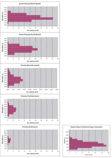
By using the USSR Glacier Inventory for each system we constructed hypsographic schemes showing the distribution of glaciated area versus altitude (Fig. 2: examples of hypsographic curves for NE Siberia). The ELA was assumed, when unknown, to be the arithmetic mean of the highest and lowest point of a glacier in the system.

10

This assumption, based on the Gefer/Kurowski method (e.g. Hess, 1904; Kalesnik, 1963), is used where glaciers are in balance with climate, which can reasonably be assumed to be the case for the USSR Glacier-Inventory data (1950s to 1970s). The area share of elevation intervals occupied with ice, is assumed at this stage of the work to linearly decrease with altitude while a glacier is retreating. These elements

15

constitute the essence of our new approach for assessing glacier-system change due to climatic fluctuations.

3.1 Precipitation/temperature data

Glacier systems analysed in this paper, represent a wide spectrum of morphology and regime types – from small corrie glaciers of the Orulgan range to large dendritic

20

glaciers of the Chersky Range and specific volcano-glacier complexes of Kamchatka. The glacier nourishment conditions also vary widely – from plentiful (monsoon type) in the eastern parts of Kamchatka (glaciers of the Kronotsky range) to insufficient on the south-east of Orulgan. The Chersky and Suntar-Khayata ranges hold an intermediate position in terms of glacier accumulation-ablation rate. Correspondingly we may expect

25

different reactions of these glacier systems to climate warming.

According to our chosen scenario the mean summer temperature would increase by between 3.1◦ _{and 4.0}◦_{N throughout the study region by 2040–2069, greatly}

exceed-TCD

Full Screen / Esc

Printer-friendly Version Interactive Discussion

EGU

ing the temperature difference between 30-year periods before and after the start of warming around 1960 (Ananicheva et al., 2002). The daily total precipitation, given by this GCM, was recalculated to solid precipitation (for the accumulation on glaciers) in monthly amounts, using the Bogdanova method (Bogdanova, 1976; Bogdanova et al., 2002), which calculates the solid-precipitation fraction according to mean monthly

5

temperature and elevation, and taking account of the model baseline and increased (projected) temperatures. In north-east Siberia under the scenario of intense warm-ing, solid precipitation would tend to grow everywhere except the Southern Massive of Suntar-Khayata. The situation on Kamchatka is the opposite: solid precipitation would decline except in the south-east, where it might increase slightly.

10

To calculate the vertical distribution of present mass-balance components we used all available climatic data, which mainly cover the second half of the Twentieth Century. This timeframe corresponds to the baseline (1959–1990) period used for reference in the ECHAM4 scenario of climate change for the next 80 years. Our baseline period approximately corresponds to the state of the glaciation reflected in the USSR Glacier

15

Inventory and partly covers the time preceding its compilation.

To complement rare meteorological-station data for high elevations (above 1000 m), we used accumulation at the mean ELA for whole glacier systems, which was cal-culated from the Glacier Inventory data or obtained from their maps (Krenke, 1982; Ananicheva and Krenke, 2005). Among glacier regime characteristics related to high

20

altitudes, ablation is considered more reliable than accumulation because it is relatively easy to calculate based on air temperature, since temperature lapse rates are easier to define and therefore better known than precipitation lapse rates (e.g. Hanna and Valdes, 2001). Accumulation is then set equal to equal to ablation of the mean ELA.

For each glacier system mentioned above, vertical profiles of ablation (A) and

accu-25

TCD

Full Screen / Esc

Printer-friendly Version Interactive Discussion

EGU

3.2 Present accumulation/ablation calculation

Accumulation was calculated based on solid precipitation measurements from meteo-rological stations; Ablation by the relationship of ablation and mean summer air tem-perature. For NE Siberia precipitation and temperature data were available only up to the height of 1400 m except for the high altitude (2068 m a.s.l.) meteorological station

5

“Suntar-Khayata”, which operated for 9 years (1957–1966) at the terminus of Glacier 31 in the Northern Massive of Suntar-Khayata Range. Based on this station’s data and data from an intermediate station at Nizhnya Baza (1350 m), located in the western slope of Suntar-Khayata Range, temperature gradients of 0.68◦_{/100 m below 1000 m,} 0.50◦

/100 m between 1000–1500 m and 0.60◦

/100 m above 1500 m were used for

sum-10

mer.

Weather stations on Kamchatka are situated within the altitude range of 100– 400 m a.s.l. In situ meteorological observations in Avachinskaya Volcano group (1963– 1974 and 1975–1979) were conducted to a height of 1500 m. The temperature gradient everywhere increases with altitude. However, inversions are not characteristic for this

15

region, in contrast to North-east Siberia (Matsumoto et al. 1999). Based on these observations, we adopted lapse rates of −0.35◦_{C/100 m between 100 and 1000 m,} −0.55◦C/100 m between 1000 and 2000 m, and −0.60◦C/100 m above 2000 m (Vino-gradov, 1975; Vinogradov and Martiaynov, 1980)

We extrapolated precipitation in NE Siberia according to the Suntar-Khayata

mete-20

orological station and in Kamchatka by pluvial gradients identified by observation at 1500 m, incorporating corrections based on accumulation (C) values at the ELA – with C defined based on its equity to ablation (A) at this level. The next step was to con-struct a corresponding vertical profile of ablation for present-day climate (the baseline period). In NE Siberia where glaciers are cold-based, the superimposed nourishment

25

prevails; therefore a significant fraction of meltwater refreezes and then melts again at the surface. In this case it is possible to use a regional variant of the global formula relating ablation to summer temperature, presented by Krenke and Khodakov 1966 In

TCD

Full Screen / Esc

Printer-friendly Version Interactive Discussion

EGU

Krenke, 1982), which was proposed by Koreisha (1991) and confirmed in calculations for Glacier 31 for reconstruction of the Suntar-Khayata glaciation during the Holocene optimum (Ananicheva and Davidovich, 2002):

A = (Tsum+ 7)3 (1)

where A is ablation in mm, and T_sum is the mean summer air temperature over the

5

glacier surface for June, July, and August.

In Kamchatka, in marine climate conditions we used a slightly modified variant of the formula (Krenke, 1982):

A = 1.33(Tsum+ 9.66)2.83 (2)

In both cases Tsumover the glacier surface (Tg) was obtained according to:

10

T_g = 0.85Tng− 1.2, (3)

where T_ng is the temperature over the rocky surrounding surface, as described in Davi-dovich and Ananicheva (1996).

The calculation of accumulation profiles consists of transformation with the help of a coefficient of concentration (Kc). The solid precipitation share for each month, and then

15

annually was defined, as explained above, by the Bogdanova method (Bogdanova, 1976; Bogdanova et al., 2002). Then, to take account of the morphological type of a glacier in the glacier system, we introduced the concentration coefficient for snow drift, avalanche snow transfer on glaciers, and its drift from volcano slopes.

According to recommendations given by Krenke (1982), in the situation where corrie

20

type glaciers prevail (such as in the Orulgan, Valagiskiy, Tumrok and Gemchen ranges) Kc is assumed to be 1.6. For the Chersky, Suntar-Khayata, and Sredinny ranges,

where medium-sized valley glaciers dominate, Kcis assumed to be 1.4. For volcanoes

covered by ice caps on the cones in combination with large valley glaciers, we used K_c as suggested as 1.4 until the cone end, and then decreased Kcfrom 1.0 to 0.6–0.7 on

25

TCD

Full Screen / Esc

Printer-friendly Version Interactive Discussion

EGU

For some glacier systems of Kamchatka we also used the mass-balance component profiles, obtained by Davidovich (2006) via the same approach. Examples of mass-balance (accumulation and ablation) curves for both Northeast Siberia and Kamchatka are given in Fig. 3.

3.3 Method of glacier change projection

5

This section of the work involved the construction of projected ablation and accumula-tion curves, Cpand Cp, for the climate of 2040–2069, based on A and N for the present

time period. For ablation/accumulation we used the assumption that the temperature shift, presented in the scenario for each grid point within which the given glacier system is located, spreads over the entire (real-surface) altitudinal range encompassed by that

10

pixel. If the glacier system is covered by a number of grid points, we used the mean value of the temperature shift.

3.4 Projected accumulation/ablation calculation

For all glacier systems considered, the mean summer temperature increase from current conditions is projected to lie within the 3.1◦_–4.0◦_{N range. These}

summer-15

temperature increases were incorporated in the calculation of ablation described above. It should be noted that we used the temperature increase at the ice-rock bound-ary because – due to microclimatic influences and the melt process – glacier surfaces depress air temperature compared with non-glacier surfaces and so experience a re-duced warming rate.

20

We used modelled daily precipitation to calculate monthly values of solid precipitation for both the baseline and projected time period using the Bogdanova (1976, 2002) method and the modeled (increased) temperatures. The purpose was to obtain ratio coefficients of solid precipitation for the projected compared with present periods for all glacier systems. Note that in NE Siberia, under the significant warming of the given

25

TCD

Full Screen / Esc

Printer-friendly Version Interactive Discussion

EGU

1.09 to 1.46) except for the Southern Massif of Suntar-Khayata (0.99). In Kamchatka the situation is the opposite: solid precipitation decreases slightly (0.74–0.96) except for the South-east where it rises slightly (1.08). Thus the southern parts of the region under consideration will be so warm that the share of solid precipitation will decrease due to the longer time period with positive temperatures.

5

For the use of these coefficients in the calculation of accumulation for the projected period, we assumed that this ratio did not change with altitude. As a result we obtained vertical curves of Npfor all glacier systems in 2040–2069.

The cross-sections with the scenario-based curves Apare taken to obtain the mean

ELA for 2040–2069 for the glacier system – ELA_p. Its shift is rarely higher than the

10

highest point of the area of accumulation (H_high) in the system (a scenario which would mean that the glaciation should disappear).

3.5 The projection of the glacier termini shift

In other cases it is assumed that after adaption of the glacier to the new climate in accordance with the Gefer method of ELA identification (according to which the ELA

15

is the arithmetic mean of the highest and the lowest glacier points; Kalesnik 1963), the elevation difference between the top of the glacier Hhighand ELAp is equal to the

elevation difference between ELApand glacier terminus (Hends). Under the assumption that the same is valid for whole glacier systems, we derive the following formula for the altitude of the lowest glacier height position:

20

H_{ends= ELAp}− (Hhigh− ELAp) = 2ELAp− Hhigh (4)

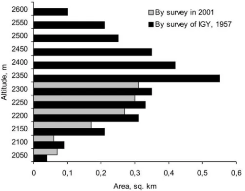
Using this equation, we obtained projected distributions of ice against altitude for the glacier systems under consideration for the period 2040–2069. Their lowest point co-incides with Hends, where glaciated area equals zero, and the highest point remains unchanged. The ice distribution of intermediate steps in elevation changes in

propor-25

tion to altitude from zero (at Hhigh) to unity (at Hends) relative to the baseline period. This assumption was based on observed data: for example, Fig. 4 shows the proportional

TCD

Full Screen / Esc

Printer-friendly Version Interactive Discussion

EGU

change of ice area by altitude for Glacier 31 (Northern Massif of Suntar-Khayata) for 1957 (the International Geophysical Year, when many such measurements began) and 2001.

Projected ice areas for the glacier systems were multiplied by A_pand C_pto derive the distribution of projected ablation/accumulation versus altitude for the climatic conditions

5

of the scenario (2040–2069). See Fig. 3, where projected balance profiles are indicated in broken line.

The comparison of the projected mass-balance components’ profiles with the eleva-tions of the “beginnings” and “ends” of glaciers with the USSR Inventory data (1940– 1970) also enables an estimation of the change of the ratio of glacier morphology types

10

and related parameters - not just glacier balance and area – under climate-change sce-narios.

4 Results and discussion

As a result of the ECHAM4 scenario described above, we obtained the following pro-jected assessments of the ELA change. The shift upward of the ELA altitude, ∆Hela, is

15

less in northern parts of NE Siberia than in the south (230 m as against 500 m in the south). In Kamchatka ∆Helaas a rule is more significant and depends on precipitation rate. The largest ∆Hela (up to 1210 m) was found in the south of Ichinskiy Volcano, located in the “rain shadow” of the Sredinniy Range (Table 1).

The change in glaciated area is anticipated to range from a complete

disappear-20

ance of some minor glacier systems, to the preservation of 70% of the present area (Kluchevskaya volcano group) and 50% of contemporary glaciated area (Shiveluch and Tolbachek volcanoes). Under the warming scenario as calculated by our approach, glaciers will not be present in southern systems of NE Siberia – southern knots of Orulgan glaciation and the Suntar-Khayata Mountains, on the Sredinniy Range of

Kam-25

chatka and around Ichinskiy Volcano. Those glaciers covering the volcanoes of SE Kamchatka and receiving intensive nourishment due to the elevation of the peaks and

TCD

Full Screen / Esc

Printer-friendly Version Interactive Discussion

EGU

proximity of the Pacific Ocean would preserve more than 40% of their area.

As for the intensity of mass exchange at the ELA, we can expect the following changes in ablation and accumulation during the projected period compared with the baseline period. ∆A,C at the ELA is greater for NE Siberia on the north of the Orul-gan, Chersky, and Suntar-Khayata ridges, where precipitation due to warming will grow

5

(Orulgan derives moisture from the Atlantic; the Chersky, while Suntar-Khayata ridges also receive moisture from the Pacific Ocean) – from 200 to almost 500 mm (accumula-tion=ablation at the ELA). In glacier systems of Kamchatka only the Kronotsky Range and volcanoes of the South-east part of the peninsula are characterized by high ∆A, C at the ELA – from 200 to 450 mm (these are areas of plentiful precipitation, and despite

10

the solid precipitation portion reducing during warming, it would still be a large abso-lute value). In the rest of the Kamchatka systems ∆A, C will range from 30 to 150 mm as a result of reduced snow nourishment because of strong warming. The glaciers of the Shiveluch Volcano attain negative ∆A, C values at the ELA due to rather abrupt decrease of the solid-precipitation fraction.

15

Judging from the glacier-balance averages both for the baseline and projected peri-ods, the glacier systems have different sensitivities to current climatic conditions and predicted future climate change. Under a constant climate, when glacier mass balance is close to zero, the glacier will not change; but assuming the same constant climate, if mass balance is positive the glacier will expand, while if it is negative it will shrink. The

20

balance trend, stability or change, and its sign are controlled by climatic conditions. A glacier can “keep up” with climate change – in this case its balance also remains near zero as well as consistent with climate. Among the glaciations considered, only that of the Chersky Range has been in this state during the baseline period. Glaciers of the Orulgan, the western slope of Sredinniy Range, the Kluchevskya Volcano group

25

and Tolbachek in Kamchatka were growing at that time. The rest have already re-treated. For the 2040–2069 period the northern knot of Orulgan glaciers and glaciers of the Kluchevskya and Tolbachek volcanoes are predicted to come into equilibrium with climate. Despite the intensive warming scenario, the Chersky glaciers will still

TCD

Full Screen / Esc

Printer-friendly Version Interactive Discussion

EGU

be consistent with climate: this is due to a combination of elevation, relief forms and corresponding glacier morphology and regime, leading to their quite slow movement and change. Glaciers of the Sredinniy and Kronotsky ranges, Shiveluch and southeast Kamchatka volcanoes will undergo accelerated retreat and provide evidence of a time lag when compared with the warming rate.

5

5 Conclusions

A new approach involving calculating the average ELA and glacier-termini level for present and projected future climate states has been used to assess glacier-system change due to predicted climate change. We have used this approach to study glacier systems with a wide spectrum of morphology and regime types from small corrie

10

glaciers of the Orulgan range to large dendritic glaciers of the Chersky Range and specific volcano-glacier complexes of Kamchatka. Glacier nourishment conditions vary widely. The reaction of these glacier systems to climate warming is found to vary con-siderably. Calculation of projected changes predict that the upward shift of ELA, ∆Hela, is less in northern parts of NE Siberia (230 m as against 500 m in the south), while

15

in Kamchatka ∆Hela as a rule is greater and depends on precipitation rate. Our cal-culations also predict the disappearance of some glacier systems, while others will preserve 70% of their present area.

Our simple, climate-based approach allows the evaluation of the behavior of moun-tain glacier systems under specified climatic scenarios for any glaciated mounmoun-tains

20

worldwide and can serve as a tool for glacier morphology and regime forecasts for the medium-term future. The originality of our approach consists in the definition of glacier-climate characteristics for a glacier system, and we have applied this here for the first time to a projection of glacier-system change. By so doing, we have derived important information about the climate sensitivity of glaciers in Northeast Siberia and

25

TCD

Full Screen / Esc

Printer-friendly Version Interactive Discussion

EGU

References

Ananicheva, M. D., Davidovich, N. V., and Mercier, J.-L.: Climate change in North-East of Siberia in the last hundred years and recession of Suntar-Khayata glaciers – Data of

glacio-logic studies – Moscow, Pub. 94, 216–225 , 2003, (in Russian with English summary and

figure captions).

5

Ananicheva, M. D. and Davidovich, N. V.: Reconstruction of the Suntar-Khayata glaciation’s in the periods of Quaternary climatic optima, Data of glaciological studies, Publ. 93, 73–79, 2002 (in Russian with English summary and figure captions).

Ananicheva, M. D. and Krenke, A. N.: Evolution of Climatic Snow Line and Equilibrium Line Altitudes- North-Eastern Siberia Mountains in the 20th Century – Ice and Climate News, The

10

WCRP Climate and Cryosphere Newsletter, N 6, July 2005, 1–6, 2005.

Ananicheva, M. D., Kapustin, G. A., and Koreysha, M. M.: Glacier changes in Suntar-Khayata mountains and Chersky Range from the Glacier Inventory of the USSR and satellite images 2001–2003, Data of glaciologic studies, Moscow, 2006, Pub. 101, 163–169, 2006 (in Russian with English summary and figure captions).

15

Bacher, A., Oberhuber, J. M., and Roeckner, E.: ENSO dynamics and seasonal cycle in the tropical Pacific as simulated by the ECHAM4/OPYC3 coupled general circulation model, Clim. Dynam., 14, 431–450, 1998.

Bogdanova, A. G.: Method of for calculation of solid and mixed precipitation proportion in their monthly standard, Data of Glaciological Studies, publ. 26, 202–207, 1976 (in Russian with

20

English summary and figure captions).

Bogdanova, E. G., Ilyin, B. M., and Dragomilova, I. V.: Application of a comprehensive bias correction model to precipitation measured at Russian North Pole drifting stations, J. Hy-drometeorol., 3, 700–713, 2002.

Davidovich, N. V.: Kamchatka glaciation during the Holocene Optimum (2006) Data of

glacio-25

logic studies, publ. 101, 221–229, 2006 (in Russian with English summary and figure cap-tions).

Davidovich, N. V. and Ananicheva, M. D.: Prediction of possible changes in glacio-hydrological characteristics under global warming: south-eastern Alaska, USA, J. Glaciol., 42, 407–412, 1996.

30

Dowdeswell, J. A. and Hagen, J. O.: Arctic ice caps and glaciers, in: Mass Balance of the Cryosphere: Observations and Modelling of Contemporary and Future Changes, edited by:

TCD

Full Screen / Esc

Printer-friendly Version Interactive Discussion

EGU

Bamber, J. L. and Payne, A. J., Cambridge University Press, pp. 527–557, 2004.

Hanna, E. and Valdes, P.: Validation of ECMWF (re)analysis surface climate data, 1979–98, for Greenland and implications for mass balance modelling of the Ice Sheet, Int. J. Climat., 21, 171–195, 2001.

Hess, H.: Die Gletscher, Brounshweig: Verlag von F. Vieweg u. S., 426 pp., 1904.

5

IPCC Second Assessment Report: The science of Climate Change 1995, edited by: Houghton, J.T., Meira Filho, L.G., Callander, B.A., Harris, N., Kattenberg, A., and Maskell, K., Cam-bridge University Press, UK, 572 pp., 1996.

Kalesnik, S. V.: Ocherki glyasiologii (Glaciological essays), Moscow, Ychpedgiz, 182, 1963 (In Russian).

10

Koreisha, M. M.: Glaciation of Verkhoyansk-Kolyima Region, Moscow, 143 pp., 1991 (in Rus-sian).

Krenke, A. N.: Mass exchange in glacier systems on the USSR territory. Leningrad, Hydrome-teoizdat, 288, 1982 (In Russia, extended English summary).

Matsumoto, K. Y., Shiraiwa, T., Yamaguchi, S., Sone, T., Nishimira, K., Muravyev, Y. D.,

Kho-15

mentovsky, P. A., and Yamagata, K.: Meteorological observations by automatic weather sta-tions (AWS) in alpine regions of Kamchatka, Russia, 1996–1997, Cryospheric studies, in Kamchatka II, Hokkaido University: Sapporo, 155–170, 1999.

Muraviev Y. D.: Present-day glaciation in Kamchatka –distribution of glaciers and snow, Cryospheric studies in Kamchatka II, Institute of Low Temperature Science, Hokkaido

Uni-20

versity, 1–7, 1999.

Shmakin, A. B. and Popova, V. V.: Dynamics of climate extremes in northern Eurasia in the late 20th century, Izvestiya AN, Fizika Atmosfery i Okeana, 42, 157–166, 2006 (In Russian, English summary and figure captions).

Vinogradov, V. N.: Present glacatiotion of the areas of active volcanism, Moscow, “Nauka”, 103

25

pp., 1975 (in Russian, extended English summary).

Vinigradov, V. N. and Martiyanov, V. L.: Heat balance of Kozelskiy Glacier (Avachnskaya Vol-cano group), Data of glacier studies, Moscow, publ. 37, 182–187, 1980 (In Russian, English summary and figure captions).

TCD

Full Screen / Esc

Printer-friendly Version Interactive Discussion

EGU

Table 1.

Change of the glacier systems characteristics in NE Siberia and Kamchatka up to the mid-21st Century (2040–2069 rr.).

Glacier system The shift of ∆Hela

(from basic to pro-jected period), m

The elevation diapa-son of the glacier system, m Glaciated area, km2, % Ablation-accumulation at the H_ela, mm Balance, cm/year Basic period Projected period Basic period, km2 Projected period, km2_(%) Basic period Projected period Basic period Projected period NE Siberia

Orulgan Northern Knot 250 750 400 7 2(27) 740 1230 +23 0

Orulgan Southern Knot 500 760 0 12 0 580 0 +14 –

Chersky – Erikit knot 320 700 200 7 1 (10) 710 1020 +7 0

Chersky-Buordakh 300 1640 1280 63 18(29) 700 1050 −2 −11 Chersky-Terentykh 300 1520 1180 28 8 (29) 720 1130 +2 + 6 Suntar-Khayata, North 350 1080 520 111 26(23) 620 850 −26 −70 Suntar-Khayata, South 500 1110 60 22 0,4(2) 460 650 −40 −30 Kamchatka Sredinny Range Eastern Slope 600 2850 2160 124 24(20) 1430 1460 −44 −170 Sredinny Range Western Slope 570 1900 1330 264 55(21) 1430 1470 +20 −44 Shiveluch Volcano 600 3240 2720 30 16(52) 1160 1080 −36 −50 Kluchevskaya Group 420 3950 3660 124 85(69) 1000 1100 +31 −4 Tolbachek Volcano 580 3085 2680 70 33(47) 1200 1350 +50 +3

Tumrok and Gemchen ranges 430 1020 0 11 0 1710 0 −81 –

Khronotsky Range 510 1150 260 91 9(10) 3350 3800 −48 −116 Valaginsky Range 610 1000 0 9 0 1400 0 −40 – Volcanows of South-Eastern Kamchatka 300 2660 2340 34 14(41) 1350 1550 −44 −60 Ichinsky Volcano 740 2080 780 29 6(22) 1510 1550 +17 +3

Ichinsky Volcano (with ac-count of blow-out from the slopes)

1210* 2080 0 29 0 1510 800* +17 –

∗ The projected elevations are higher than the real topography, so the glaciation in these cases will not exist under the scenario used.

TCD

Full Screen / Esc

Printer-friendly Version Interactive Discussion

EGU

TCD

Full Screen / Esc

Printer-friendly Version Interactive Discussion

EGU

460

Fig. 2. Examples of hypsographic curves (distribution of ice area via altitude) for NE Siberia

TCD

Full Screen / Esc

Printer-friendly Version Interactive Discussion

EGU

Fig. 3. Vertical profiles of ablation and accumulation for baseline/present (solid lines) and

projected by ECHAM scenario for 2040–2069 (broken lines) for two different glacier systems:

(a) Northern massif of Suntar-Khayata (NE Siberia); and (b) Kluchevskaya volcano group of

glaciers (Kamchatka). The method of construction of these profiles is explained in detail in the main text.

TCD

Full Screen / Esc

Printer-friendly Version Interactive Discussion

EGU

475

Fig. 4. Distribution of ice area via altitude of Glacier 31 (Suntar-Khayata Range) derived from