How can remote sensing contribute in groundwater modeling?

How can remote sensing contribute in groundwater modeling?

P. Bauer-Gottwein&W. Kinzelbach

Abstract Groundwater resources assessment, modeling and management are hampered considerably by a lack of data, especially in semi-arid and arid environments with a weak observation infrastructure. Usually, only a limited number of point measurements are available, while groundwater models need spatial and temporal distribu-tions of input and calibration data. If such data are not available, models cannot play their proper role in decision support as they are notoriously underdetermined and uncertain. Recent developments in remote sensing have opened new sources for distributed spatial data. As the relevant entities such as water fluxes, heads or trans-missivities cannot be observed directly by remote sensing, ways have to be found to link the observable quantities to input data required by the model. An overview of the possibilities for employing remote-sensing observations in groundwater modeling is given, supported by examples in Botswana and China. The main possibilities are: (1) use of remote-sensing data to create some of the spatially distributed input parameter sets for a model, and (2) constraining of models during calibration by spatially distributed data derived from remote sensing. In both, models can be improved conceptually and quantitatively.

Résumé L’évaluation, la modélisation et la gestion des ressources d’eau souterraine sont considérablement entra-vées par un manque de données, particulièrement dans les régions semi-arides et arides possédant peu d ’infrastruc-tures d’observation. Généralement, seul un nombre limité de points de mesure sont disponibles, alors que les modèles hydrogéologiques demandent des distributions

spatiales et temporelles de données d’entrée et de calibration. Si de telles données ne sont pas disponibles, les modèles ne peuvent pas jouer leur rôle d’appui à la décision puisqu’ils sont notoirement de mauvaise résolu-tion et incertains. De récentes avancées en télédétecrésolu-tion constituent de nouvelles sources pour les données spatiale-ment distribuées. Comme les entités utiles telles que les flux et les niveaux d’eau ou les transmissivités ne peuvent pas être observées directement par télédétection, il con-vient de trouver des moyens de relier les quantités observables aux données d’entrée nécessaires aux mod-èles. A travers des exemples au Botswana et en Chine, un aperçu des possibilités d’utilisation des observations issues de la télédétection en modélisation hydrogéolo-gique est présenté. Les principales possibilités sont: (1) l’utilisation de données de télédétection pour créer une partie des données d’entrée spatialement distribuées d’un modèle, et (2) la contrainte des modèles lors de la calibration avec des données spatialement distribuées dérivées de la télédétection. Dans les deux cas, les modèles peuvent être conceptuellement et quantitative-ment améliorés.

Resumen La evaluación, modelizado, y gestión de recursos de agua subterránea, se dificulta considerable-mente por la falta de datos, especialconsiderable-mente en ambientes áridos y semi-áridos donde existe una infraestructura débil de vigilancia. En esto ambientes normalmente solo se cuenta con un número limitado de mediciones puntuales mientras que los modelos de agua subterránea necesitan distribuciones temporales y espaciales de datos de entrada y calibración. Si estos datos no están disponibles los modelos no pueden jugar su rol apropiado en el apoyo de decisiones ya que en estas circunstancias son bastante inciertos e indeterminados. Los desarrollos recientes en sensores remotos han abierto nuevas fuentes para datos con distribución espacial. Debido a que las entidades relevantes tal como flujos de agua, presiones o trans-misividades no pueden observarse directamente mediante sensores remotos, tienen que encontrarse maneras para vincular las cantidades observables a datos de entrada que requiere el modelo. Se proporciona una revisión de las posibilidades de utilizar observaciones de sensores remo-tos en los modelos de agua subterránea apoyándose en ejemplos de Bostwana y China. Las dos posibilidades son: (1) uso de datos de sensores remotos para crear algunos de Received: 24 March 2006 / Accepted: 19 October 2006

Published online: 25 November 2006 ©Springer-Verlag 2006

P. Brunner

:

:

:

Institute of Environmental Engineering, ETH Zurich,

Zurich, Switzerland

e-mail: Kinzelbach@ifu.baug.ethz.ch P. Bauer-Gottwein

Institute of Environment and Resources, Technical University of Denmark, Lyngby, Denmark

los parámetros de entrada distribuidos espacialmente para un modelo, y (2) restricción de modelos durante la calibración mediante datos distribuidos espacialmente obtenidos de sensores remotos. Para ambas posibilidades los modelos pueden mejorarse conceptual y cuantitativamente.

Keywords Remote sensing . Numerical modeling . Geophysics . Spatial data analysis . Model calibration

Introduction

The term remote sensing should not be confined to Earth observation systems with sensors measuring in the visible, infrared and radio wave regions of the electromagnetic radiation spectrum. It also includes geophysical surveys of gravity, magnetics, and electromagnetics. Only the geo-physical surveys offer the possibility of exploring the subsurface. Remotely sensed data can be obtained from various platforms such as satellites, airplanes, drones, blimps and masts. The ways in which remote sensing can contribute to groundwater modeling are so numerous that this review paper can by no means cover all aspects. The selection is based on the authors’ experiences. Other aspects are covered, for example, in Becker (2006).

Regional hydrological models such as groundwater models require distributed input data. Classical hydrological measurements provide only point data obtained for example at a weather station, a gauging station, or a borehole. One of the main problems in hydrological research today is how to pass from point information to regional distributed informa-tion. Remote sensing offers a possibility to do this for certain parameters required in groundwater modeling. In principle, the patterns from remote sensing can be translated into a deterministic distribution of input data on a cell-by-cell basis or in the form of zones. Even if absolute values of these data are uncertain, they still reduce the degrees of freedom of the model and thus lead to a better posed inverse problem and a robust solution. Remote sensing is, therefore, an extremely useful tool in the acquisition of spatially distributed data for modeling. All raw remote-sensing data present spatial patterns which can be related to features or processes above the surface (such as clouds), on the surface (such as evapotranspiration), or in the shallow subsurface (such as electrical conductivity). However, the parameters directly accessible by remote sensing are often not the ones required in groundwater models. This means that the utilization of remote-sensing data requires another modeling step to convert them to data usable as input data or verification data in spatially distributed models (e.g. Kemna et al.2002). It is the combination of the pattern information with the point information at ground observation stations that allows spatial distributions of the parameter in question to be obtained. The correlations between ground measurements and remote-sensing data are subject to noise. Such stochastic relationships can, however, still be utilized in the conditioning of stochastic models and data assimilation. Take precipitation as an example for a distributed data set. From remote-sensing data such as cloud temperature

distributions (e.g. Herman et al.1997) or weather radar data (e.g. Collier2002) on drop spectra, estimates of precipita-tion can be derived through a model. The resulting distribution of precipitation is uncertain as far as absolute values are concerned, while the relative intensities are much more reliable. If the resulting distribution is scaled with precipitation measurements obtained at stations on the ground, a map of absolute precipitation quantities results which is superior to maps obtained from the mere mathematical interpolation of station data.

In regions where spatial observation networks are extremely dense, remote sensing may be of less interest. However, the main water problems of today are in developing regions of the world with weak infrastructure, low accessibility, and data scarcity. It is in such cases that remote sensing can develop its largest use for water resources management. Combined with traditional meth-ods remote sensing has a great potential in improving the quality of modeling work.

In the following sections, the types of information which can be extracted from remote sensing are described. Then four examples illustrate ways of using this informa-tion in groundwater modeling. These examples include: – The direct construction of an input data set (aquifer

thickness)

– The reduction of degrees of freedom in inverse groundwater modeling

– The calibration of a groundwater model by pattern information on a quantity that can both be measured by remote sensing and calculated from the model

– The conditioning of a stochastic groundwater model with noisy input data from remote sensing

What information contained in remote-sensing

images is of potential use in groundwater modeling?

Airborne geophysical surveys allow for the identification of faults and dikes, changes in lithology and the depth of magnetic features (e.g. Danielsen et al. 2003; Doll et al. 2000; Jorgensen et al. 2003a,b; Thompson 1982). This information is helpful in constructing more realistic conceptual models of aquifers. An aquifer that is compartmentalized by dikes and faults will behave differently from an aquifer without such flow guides.

Geomagnetic surveys have, up to now, mainly been used in the search of Earth resources of high economic value such as minerals and hydrocarbons. However, once acquired, the geophysical data retain potential for many other applications including groundwater exploration and management (LaBrecque and Ghidella 1997). Botswana, for example, has embarked on airborne high-resolution magnetic surveys to cover the whole country, the primary aim being the exploration of formations bearing diamonds and other minerals (MFDP 2003). Hydrogeologists in Botswana are now beginning to benefit at almost no cost from the data acquired (e.g. DWA2004,2006).

Lineaments on the surface have been identified early as conduits for groundwater flow in fractured aquifers and hence targeted for locating production wells. Their use in geology is already widespread (e.g. Lattmann 1958; Meijerink 1996; Tam et al.2004).

The overlaying of lineaments mapped from conven-tional remote-sensing techniques (aerial photographs and satellite images) and those derived from airborne geophysical methods can be implemented using geo-graphical information systems (GIS) at both local and regional scales. Some lineaments detectable by airborne geophysics may be due to deep-seated sources (up to several tens of kilometers) and hence have no effect on groundwater flow in aquifers of interest, which are mostly within a few hundreds of meters below the ground surface. Therefore, the depths to magnetic sources must be estimated in order to retain only linea-ments that are deemed relevant to groundwater flow. On the other hand, lineaments identified with conventional methods give only information on structures with surface expression and no information on depth and vertical continuity of the structures.

Space-borne gravitational surveys such as the Gravity Recovery and Climate Experiment (GRACE) mission can be used to detect temporal changes in the total water storage (surface water, soil water and groundwater). A 2-cm thick, infinitely extended layer of pure water located at any depth below a gravimeter generates an incremental gravitational acceleration of 1×10−8 m/s2 or 1 μGal (microgal). The temporal change in total water storage (TWS) in the Earth system is therefore directly propor-tional to the temporal change in the measured gravitapropor-tional acceleration. The potential of time-lapse gravity surveys to monitor the status of water resources systems has been recognized for a long time. Ground-based time-lapse gravity surveys were used successfully to determine alluvial aquifer storage and specific yield, which is a key parameter for the sustainable management of groundwater resources (Pool and Eychaner 1995). Moreover, it has been demonstrated that superconducting ground-based gravimeters reflect hydrological signals on the order of several microgals (Amalvict et al. 2004; Bower and Courtier1998; Neumeyer et al. 2006). The GRACE twin satellites have dramatically improved the accuracy and resolution of regional observations. This satellite mission delivers an accuracy of 0.4 μGal or 1 cm of groundwater on spatial scales larger than 1,300 km (Andersen and Hinderer2005; Andersen et al.2005) and delivers reliable observations of the regional part of the global hydrological cycle. Although the spatial resolution is still less than the size of typical groundwater systems, the prospects of this method for future use in verification of models, especially for the determination of the storage coefficient, are bright. For a phreatic aquifer, the surface of the terrain is also the upper boundary of the aquifer and constrains the groundwater levels. Surface elevations can be determined by various remote-sensing techniques, from airborne platforms (e.g. light detection and ranging LIDAR (Bufton et al. 1991), interpretation of stereo orthophotos (Kaab

2002), or satellite platforms using, for example, radar interferometry (Madsen et al. 1993; Rabus et al. 2003; Slater et al. 2006; Zebker and Goldstein 1986). In the latter case, the phase differences in pixels seen from different points in orbit allow a translation into differences in elevation. To obtain absolute elevation data and to verify their relative distribution, accurate elevation data at ground control points are required. These can be obtained, for example, with differential GPS (global positioning system). In many applications, the depth to groundwater is of importance for environmental reasons, including water supply to vegetation or salinization by phreatic evapora-tion. This distance is the difference between the surface elevation given by the digital elevation model (DEM) and the groundwater level.

Several preprocessed DEMs are available. A recent one is the shuttle radar topography mission (SRTM) data set, a DEM covering all land areas between 60°N and 56°S latitude at a 90-m pixel resolution and a vertical accuracy of at best 5 m (Rodriguez et al.2005; Slater et al.2006). While the spatial resolution is sufficient for most groundwater applications, the vertical accuracy is not. Only LIDAR can presently supply a sufficient vertical accuracy and spatial resolution to determine reliable depths to groundwater. However, new missions aiming to acquire a global DEM with very high accuracies and fine resolution are currently being developed, e.g. Tan-DEM-X (Microwave and Radar Institute 2006; launch planned for 2009). If radar or LIDAR techniques cannot be applied, be it for cost or for accuracy reasons, correlations between vegetation type, vegetation density or other land surface characteristics reflected in multi-spectral satellite images on one hand, and topographic elevation on the other, can be exploited. In some cases, particularly in wetlands, topography can be inferred from land-cover maps at an accuracy not reached with radar interferometry (Gumbricht et al.2005).

High-precision measurements of the surface elevation changes can reveal regional subsidence caused by piezo-metric depression around wellfields (e.g. Hoffmann et al. 2001) or seasonal variations of the groundwater level (Chang et al. 2004). Once a relation is given between subsidence and drawdown, a spatial distribution of drawdown can be obtained from the amount of surface subsidence observed. Differential GPS can also serve the purpose of determining temporal variations in the ground level related to groundwater pumping or recharge. This information is, however, again point like.

Finally, river and lake levels can be determined by using radar satellites (e.g. Berry et al. 2005; Jekeli and Dumrongchai2003). Such data are available close to real time, for example, see European Space Agency work on rivers and lakes (ESA2005). Lake and river levels can be of relevance for subsurface hydrology if they are indicative of groundwater levels.

The bulk of remote-sensing data relevant for ground-water modeling are data that allow for quantification of the distribution of recharge or discharge. Recharge is one of the most important quantities for sustainable

ground-water management. In dry regions, its estimation has been, up to today, a challenge, as it may occur only sporadically at intervals of several years. It may also be spatially very heterogeneous due to the distribution of precipitation, soil properties, water use by plants or runoff processes. One of the earliest applications of remote-sensing relevant in hydrology was the characterization of vegetation type, density and its status (e.g. Fensholt et al. 2006). This information is also of interest as a proxy for evapotrans-piration (e.g. Loukas et al. 2005). Vegetation may be an indicator for the presence of water and the depth to groundwater level.

Forflat terrain, the groundwater recharge potential over long time intervals is the long-term average residual between precipitation P and evapotranspiration ET. Both quantities can be estimated from remote-sensing data. The precipita-tion can be estimated from cloud temperature data by certain algorithms (e.g. Herman et al.1997) in combination with precipitation data from meteorological stations on the ground. The Famine Early Warning Systems Network (FEWS 2006) offers such data at a 10-day temporal resolution for all of Africa. Evapotranspiration can be derived from multispectral satellite data via a surface energy balance. To put it simply, a dry pixel will heat up to higher temperatures than a pixel which has a large amount of water available for evaporative cooling. In this sense, radiation data can be related to evapotranspiration. The fraction of net radiation energy consumed by evaporating water can be estimated with different methods. In SEBAL (surface energy balance algorithm for land; Bastiaanssen et al. 1998a,b), the energy fluxes in the surface energy balance are calculated explicitly, while in a simplified method described by Roerink et al. (2000), this fraction is determined from a pixel-wise plot of surface temperature versus albedo. Other methods use different dimensions of the feature space instead, e.g. the Normalized Difference Vegetation Index (NDVI), which is a measure of the vigor of vegetation growth (Sandholt and Andersen1993).

Unfortunately, both ET and P obtained from remote sensing are inaccurate. Calculating the difference, P–ET, leads to error propagation, especially when both quantities are of similar magnitude. This is often the case in semi-arid and semi-arid areas. Still, the spatial patterns of P-ET may be of help in regionalization of traditional point measure-ments of recharge, e.g. obtained with the chloride method (Brunner et al. 2004).

The spatial distribution of recharge may be very heterogeneous even if the distribution of precipitation is homogeneous. If water collects and infiltrates in depres-sions, those may dominate the total recharge of an area. This process has been documented in Niger (Leduc et al. 2001). Water surfaces forming in the landscape and their temporal behavior can be identified by remote sensing, e.g. via radar or multi-spectral characterization (e.g. McCarthy et al. 2003; Roshier and Rumbachs 2004). Their density and distribution are indicative of the spatial distribution of recharge.

In wetlands, the interaction between surface water and groundwater is crucial for the understanding of the

wetland behavior. The development of water surfaces andflooding patterns over time is, in this case, a valuable data set for model calibration (Bauer et al.2006a,b).

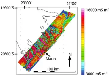
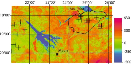
Groundwater recharge from rivers, streams and wet-lands, under certain circumstances, can also be inferred from remote sensing through anomalies in temperature or electrical conductivity. In arid environments, evaporation is mostly through plants in the form of transpiration. This increases salinity in groundwater and hence electrical conductivity. The freshly infiltrated water beneath a stream, in contrast, has a low electrical conductivity. The varying electrical conductivity of the underground can be detected by airborne electromagnetic methods (e.g. Paine and Collins2003). On the fringes of the Okavango Delta, Botswana (Fig. 1) the variations in groundwater salinity could be seen clearly from an airborne electromagnetic survey (Fig.2). Sattel and Kgotlhang (2004) also used this approach for salinity mapping in the Boteti area just south of the Okavango Delta. The data was validated by ground geoelectrical methods and drillhole information.

In arid and semi-arid areas, the discharge of groundwater via direct evaporation from the water table and evapotrans-piration by trees may account for most of the discharge of an aquifer. Discharge via a draining stream, as in a humid zone, rarely occurs. The estimation of discharge via trees has been the subject of remote-sensing studies looking both at ET derived from energy balance calculations as well as single tree counts according to species and canopy size and combining this remote-sensing information with informa-tion on the single tree, e.g. obtained from sap flow measurements (e.g. Lubczynski and Gurwin2005).

Salt crusts indicate high water tables with phreatic evaporation. They can be mapped by multispectral satellite data and used as an indicator for phreaticfluxes and depth to groundwater (e.g. Metternicht and Zinck 2003; Brunner et al.2006).

Soil-water balance calculations as a function of time require data in addition to average ET and P to account for water storage in the soil. A soil-water balance model requires some information on the field capacity of a soil which could be estimated on the basis of the soil type. Here, hyperspectral satellite information can help (e.g. Chabrillat et al. 2002; Leone and Escadafal 2001; Shepherd and Walsh 2002; Ben-Dor et al. 2004) as well as gamma radiation counts from airborne platforms (e.g. Cook et al. 1996) indicating clay content (e.g. Rainey et al. 2003). Soil moisture itself and its temporal variation may in the future be accessible from passive and active microwave sensors. A mission planned for early 2007 by ESA has been designed to observe soil moisture over the Earth’s land mass. It has to be stressed though that the moisture seen relates only to the top centimeters and the use of this data type requires substantial modeling. For more information, see also Becker (2006).

The vegetation vigor derived from multi-spectral satellite data can be used as an indicator for irrigation and can, therefore, be employed as a relevant parameter in monitoring the irrigated areas and for timing of irrigation (Droogers and Bastiaanssen 2002). The main application

of remote sensing of hydrological variables already in operative use today is the scheduling of irrigation.

General process of applying remote-sensing data

in groundwater modeling

Groundwater models are based on the flow equation

S0@h

@t ¼ r Krhð Þ þ w

where S0is the storativity, h the hydraulic head, t is time,

K the hydraulic conductivity tensor and w the distribution of sources and sinks. Together with boundary conditions in space and time, theflow problem is uniquely defined. The equation and boundary conditions contain the spatially distributed functions of hydraulic conductivity, storativity, and recharge. Via those distributions as well as the boundary conditions, the geometry of the aquifer is defined. In general, only limited information on the spatial distribution of these input parameters is available. Yet, a model computation needs a complete set of parameters. There are different ways to determine or estimate those. In traditional model calibration, the aquifer is divided into a limited number of zones. Within these zones, aquifer properties are assumed to be constant. This means a strong reduction in degrees of freedom. The zonation should be such that the parameters are expected to show little spatial variation within the defined zones. Remote sensing can play a role in the definition of these zones. For subsurface features, structural elements as seen in areal geophysical surveys together with point data from drillings and pumping tests allow zoning. So the first main use of remote-sensing data is seen in the spatial modulation and

interpolation of input data, where otherwise a homogeneous value or a purely mathematical interpolation function would have to be used. During the process of model calibration, updated estimates of the missing parameters such as hydraulic conductivity (for the defined zones), are obtained such that a historical record of head and/orflux observations can be reproduced. This process is non-unique.

Piezometric head data do not reduce the uncertainty of the estimated parameters of storativity, hydraulic conduc-tivity and recharge, in case those parameters are only known within large error intervals. If, however, the spatially distributed input data can be constrained, the calibration problem stabilizes. Let us assume the spatial

Fig. 2 Shallow subsurface electrical conductivity map from an airborne electromagnetic method. The study area is outlined in Fig. 1b. The black lines represent the border (consisting of channels) of the Delta

Fig. 1 a Locations of the study sites in Botswana, b Okavango Delta, Kavimba, and c Kanye. The black box in b along the fringes of the Okavango Delta represents the study area discussed in Fig.2b. The background of the images (b and c) repre-sents patterns of evapotranspi-ration (annual average). Red stands for high, green for moderate and blue for low evapotranspiration rates. The black lines represent interna-tional borders

distribution of relative recharge can be estimated from land use and soil type. And let us further assume that the yearly regional variation can be estimated from local lysimeter data. Then the total function of recharge in space and time R(x,t) could be reconstructed as the product of the temporal-spatial average of recharge R_av, a weighting factor f(x) expressing the relative values on areas with different land use and a weighting factor g(t) expressing the relative proportion of recharge in a certain time interval, i.e.

R xð Þ ¼ R; t avf xð Þg tð Þ

If f(x) can be obtained from remote-sensing data and g(t) can be determined from point data at a few lysimeters there is only one unknown parameter left and the large number of degrees of freedom residing in a temporal-spatial distribution collapses into one single number, the temporal-spatial average value Rav.

Alternatively, remote-sensing information on properties such as recharge could also be introduced in the traditional model calibration in the form of prior knowledge. As Carrera and Neuman (1986) show, ill-posedness of the model calibration can be mitigated by prior knowledge about the parameters to be estimated. Remote sensing can even be introduced as a kind of soft (not exact) information into the traditional zone based model calibra-tion strategy.

A more modern strategy of obtaining model parameters is the stochastic modeling approach. It acknowledges that all parameters are uncertain due to heterogeneity and/or measurement errors. Instead of a single best parameter set, a large ensemble of possible parameter sets is determined using stochastic information. This procedure also allows quantification of the uncertainty of the model results.

Remote-sensing information intrinsically contains un-certainty because the correlation between remote-sensing patterns and ground truth will not be perfect. The stochastic modeling approach is able to use this type of information. The remote-sensing-based data and ground truth can be used to generate a series of equally likely images of the variable of interest within the uncertainty of the correlation. The co-located co-simulation algorithm, developed in the geostatistical community (Almeida and Frykman 1994), is suited for this purpose as it is especially designed to handle exhaustive data on a regular grid. This algorithm simplifies the relation between the remote-sensing data and the variable of interest to a linear correlation coefficient (Markov assumption) (e.g. Goovaerts 1997). The generated images are conditioned to the two different data sources, and take into account their estimated errors, a (linear) correlation between them, and a variogram estimated from the spatially distributed remote-sensing data. These equally likely images of the variable of interest sample the high-dimensional space of possible spatial distributions of the variable of interest within the uncertainty bounds mainly given by the mismatch between remote-sensing data and ground truth. In a case where the resolution of the

hydrological model coincides with that of the remote-sensing raster, and further, if the remote-remote-sensing data are perfect (perfect correlation between variable of interest and the measured signal), this space of possible spatial distributions would be reduced to one deterministic “truth”. As this truth will never be known, the stochastic calibration of a groundwater flow model consists of the selection of an ensemble of realizations of input data (combined from stochastic and deterministic information), which reproduce hydraulic head, flux and possibly tracer data to a predefined degree.

There are different ways to proceed. An extremely large amount of equally likely realizations (millions) of the variable of interest can be generated in the way described before and processed through the hydrological model, until enough realizations have been found that are consistent with the hydraulic head, flux, and possibly tracer data. The disadvantage is that this is very inefficient, especially for strongly non-linear models. In case of conceptual model errors, no valid solutions will be found. Alternatively, a limited number of realizations (hundreds) of the variable of interest can be generated and inversely conditioned to the observed hydraulic head data and tracer test data by a Monte-Carlo-based stochas-tic inverse conditioning approach. These methods have been developed to accommodate more qualitative facies pattern data obtained from outcrops. Examples are the sequential self-calibration method (e.g. Gómez-Hernández et al. 1997; Hendricks Franssen 2001), the pilot point method (e.g. LaVenue et al. 1995) or the representer method (e.g. Valstar et al.2004). The inverse conditioned realizations are conditional to hydraulic head data, tracer test data and the direct measurements of the variable of interest, but not necessarily to the remote-sensing infor-mation, as the relationship between the remote-sensing data and the variable of interest cannot be handled by these algorithms. However, for all these algorithms, the remote-sensing information would be preserved in some way in the inverse conditioned realizations.

In the literature, some approaches are presented that partially circumvent the problem. A possibility is to constrain the variogram of the variable of interest in the inverse-modeling procedure (Oliver et al.1997). However, this does not preserve the full information potential of the remote-sensing image, as it only considers area-averaged two-point statistics. Capilla et al. (1999) developed the method of conditional probabilities, which includes exhaustive soft information in the sequential self-calibra-tion procedure by perturbing the condiself-calibra-tional probabilities (conditioned to the exhaustive soft information as well) instead of directly perturbing the values for the variable of interest. Also, this approach has some drawbacks: a large number of indicator variograms has to be inferred, and the indicator variograms are area-averaged two-point statis-tics. In addition, the perturbation of the image is only constrained by the inferred univariate local-conditional probability density functions. Hendricks Franssen et al. (2006) modify the sequential self-calibration approach and introduce an extra term in the objective function that

penalizes a too strong deviation between the calibrated pattern for the variable of interest and the satellite information related with the variable of interest. This method does not need to make the stationarity assumption. Other geostatistical methods require that the spatial distributions are stationary. The method, however, allows any kind of remote-sensing information to be included in groundwater models that are available as exhaustive gridded information, and that show a correlation with a variable of interest (e.g. recharge rate, aquifer thickness). Notice that a critical step in the methodology consists of establishing the (statistical) relationship between the remote-sensing signal and the values for the variable. Together with the statistical relation, the uncertainty of the established relation should also be quantified.

Example: aquifer thickness of the Okavango Delta,

Botswana

The Okavango Delta is a wetland system of about 20,000 km2 area situated in the northwest of Botswana. A recently published integrated hydrogeological model of the Okavango Delta (Bauer et al. 2006a,b) assumes, in a simplifying approach, that the Kalahari Sands aquifer underlying the Delta has a uniform thickness over the whole model domain. A more realistic distribution of aquifer thickness beneath the Delta can be obtained from semi-automated interpretations of aeromagnetic data. The high quality aeromagnetic data available in Botswana (collected at ~250-mflight line spacing) mostly record the magnetic effects of metamorphic and igneous basement rocks and dikes immediately underlying the generally non-magnetic sedimentary cover, including the Kalahari Sands aquifer. Since erosion resulted in a relatively smooth surface prior to deposition of the unconsolidated sedimentary cover, the depth to the top of magnetic rock at any location is likely to be a good estimate of sedimentary cover thickness.

The semi-automated estimates of depth-to-magnetic sources are based on the 3D Euler deconvolution technique (e.g. Reid et al. 1990; Mushayandebvu et al. 2001), which requires knowledge of the magnetic field spatial derivatives and the so-called structural index term (an indication of the power to which a magnetic anomaly decays as the inverse of distance from its source). In the computations, it was assumed that the majority of sources can be adequately represented by dike-like models. This is clearly valid for the hypabyssal dikes, but it is also a good approximation for those regions where the magnetic anomalies are caused by moderate- to steep-dipping faults or the limbs of tight peneplained folds.

Figure3a shows the structural pattern as extracted from the aeromagnetic data. Blue text on the map shows thickness of sands from drillholes, whereas the colored symbols indicate lithological units. Figure 3b shows the interpolated thickness of the Kalahari Sands below the Delta. It can be seen from these twofigures that the thick-ness of the aquifer is structurally controlled. Ground truth

(i.e. depth from drillholes) and depths determined from remote sensing correlate well (correlation coefficient of 0.9).

Example: compartmentalization of the Kanye aquifer,

Botswana

The dolomites in the Kanye region of Botswana (Fig.1c) constitute an aquifer ideal for groundwater abstraction. They are fed by recharge through fractures. Recharge studies carried out with the chloride method showed that in parts of the aquifer, 25 mm/a is realistic (Gehrels and Van der Lee1990).

A model of the aquifer, constructed by a consultant (DWA2000), containing a large number of transmissivity zones, was able to reproduce measured heads very accurately. This is not surprising, given the large number of calibration parameters used. This model, however, failed in its predictions for the viability of pumping wells. Wellfield operation with the sustainable pumping rates predicted by the model led, in reality, to huge drawdowns and some wells fell dry. The uncertainty of recharge is not large enough to account for the failure of the prediction.

An analysis of lineaments identified by using aero-magnetic, aerial photographs and satellite images suggests that the Kanye aquifer is strongly compartmentalized by intrusion dikes. Another observation hints that the aquifer is compartmentalized. The general piezometric head map shows a ridge of piezometric maxima with heads decreasing from the ridge in all directions. CFC (chlorofluorocarbons) concentrations, however, show that water in boreholes with high piezometric heads is older than water in boreholes with lower heads (Klump et al. 2004). That means the direction of flow lines does not coincide with the direction of increasing water age.

A conceptual model of the aquifer which is not in contradiction with the observations can be built on the basis of surficial lineaments and magnetic anomalies. Figure 4 shows features from the geomagnetic survey, aerial photographs and Landsat imagery. Highly magnetic areas (red, in Fig. 4a–c) are volcanics, granites, syenites and dolerites. Weakly magnetic areas (blue, in Fig.4a–c) are dolomitic and quartzitic areas. Major lineaments are clearly visible and their high magnetic signal suggests that these are fractures intruded by dolerite dikes. Indeed both ground mapping and borehole information confirm that these lineaments are intruded by dolerite dikes. In the conceptual model, only these major lineaments are included asflow barriers. Even if these major lineaments were not intruded by dolerite, large fractures are often filled with very fine material or silicified and, therefore, still act asflow barriers. The dike structure entered into the model is shown in Fig. 4f.

The dikes were analyzed with respect to their depth and the relative depth of water strikes in their vicinity. On the basis of these criteria three categories of dikes with three different transmissivities were defined.

The water strikes in the northern part of the Kanye aquifer are generally much deeper (average 80 m below ground level) than the top of the dikes while in the southern part they are in the same depth range. Therefore, a low hydraulic conductivity value (2×10−9 m/s) was assigned to the dikes in the northern part, while a larger value (2×10−7m/s) was assigned to the dikes in the south with the remaining dikes having an intermediate value (1.5×10−8m/s).

The transmissivities of the model zones between dikes (compartments) were assigned as homogeneous using the pumping test values available in that compartment. The three unknown dike transmissivities were used as sole degrees of freedom for calibration of 38 heads in the steady-state pre-pumping case. As only the product of dike hydraulic conductivity and thickness is relevant, thickness was kept constant at 1 m. Recharge zonation was done on the basis of patterns of potential recharge obtained from remote sensing. The pattern was scaled to accommodate the few recharge estimates available. Even with the small number of calibration parameters, a very good fit resulted. Huge, unsustainable drawdowns were predicted by the new model when simulating the influence of the recommended abstraction rates from the old model. It was thus evident why most pumping wells

started to fall dry 1 year after the pumping operations commenced. While the regional recharge is still consid-erably larger than the total pumping rate, well fields within a compartment cannot utilize the regional recharge because the dikes limit the amount of waterflowing to the wellfield.

Example: phreatic evaporation and soil salinization,

Yanqi Basin, China

The agriculturally highly productive Yanqi Basin (located in the Xinjiang Uygur region of China, Fig.5) is mainly irrigated with water drawn from the riversflowing through the basin. The intensive agriculture has led to several environmental problems, especially soil salinization. A groundwater model simulating the influence of irrigation Fig. 3 Determination of aquifer thickness from airborne magnetic

survey. a Structural patterns extracted from aeromagnetic data. The orange outline represents the boundary of the study area. The thin solid black line represents the boundary of the Okavango Delta.

The thick black lines represent faults (triangles point in the direction of throw). The dotted lines also represent faults (with unknown throw direction). b Estimated thickness of Kalahari Sands aquifer in m

„

Fig. 4 Combination of aeromag data and lineament data to arrive at flow barriers implemented in the groundwater model of the Kanye aquifer. a Total magnetic intensity, bfirst vertical derivative, c analytic signal. Red signifies highly magnetic areas and blue signifies weakly magnetic areas. d Lineaments from aerial photos, e lineaments derived from Landsat image, f flow barriers imple-mented in the model; the red line represents the model boundary

on the basin’s water and salt balance was constructed and verified by using spatially distributed input data derived from remote sensing. The most interesting spatial data set derived from remote sensing is the distribution of phreatic evaporation, i.e. the direct evaporation from the water table. This quantity can be both determined from remote sensing and calculated directly by the model. The separation of phreatic evaporation from transpiration is important- the two quantities are related in different ways to the salt balance of the Yanqi Basin.

The map of phreatic evaporation was constructed by combining remote-sensing images and measurements on the ground. Using the US National Oceanic and Atmo-spheric Administration’s Advanced Very High Resolution Radiometer (NOAA-AVHRR) images, the spatial distri-bution of evapotranspiration (ET) was obtained by the method of Roerink et al. (2000). However, this distribu-tion represents the sum of transpiradistribu-tion from vegetadistribu-tion and of phreatic evaporation. In the Yanqi Basin, transpi-ration occurs only on irrigatedfields. Phreatic evaporation, however, occurs in irrigated and non-irrigated areas. On the basis of stable isotope profiles obtained in the unsaturated zone, phreatic evaporation can be determined (Barnes and Allison 1988). Phreatic evaporation E was determined at seven non-irrigated ground stations. The difference between ET determined from the NOAA-AVHRR images and phreatic evaporation E is the transpiration rate T of vegetation: ET–E=T.

In this notation, transpiration also includes the evaporation of the irrigation water stored above the zero flux plane and not being consumed by plants. If a correlation between the transpiration rates T calculated with this equation and the NDVI can be found, the NDVI, can be used to map transpiration. Such a correlation has been established (R2=0.80). The resulting map of T was calculated according to this correlation (Brunner 2005).

The calibration strategy for the groundwater model was that all external fluxes of the aquifer were specified and only leakances and hydraulic conductivities were adjusted. Besides the comparison between calculated and observed river discharge at seven locations and the residual between

observed and calculated depths to groundwater, the groundwater model was verified with the remotely sensed map of phreatic evaporation (Fig.6).

Example: constraining of model calibration by using

a DEM and recharge potential from remote sensing,

Kavimba, Botswana

Kavimba is situated in the Chobe District in the northeast of Botswana (Fig. 1). One option for a long-term sustainable water-supply scheme is groundwater abstract-ed from the establishabstract-ed Kavimba well field. Concerns were raised on the sustainability of this option, given the semi-arid to arid climatic conditions. A model study was performed to estimate the average yearly recharge rate and the risk of overpumping the aquifer.

Fig. 5 Location of the Yanqi Basin. The background image is a color composite based on Landsat data

Fig. 6 Comparison between phreatic evaporation calculated with the groundwater model (a) and phreatic evaporation obtained from the remote sensing (b) in mm/a. The thin black lines represent the drainage net of the Basin

Hendricks Franssen et al. (2006) applied a stochastic inverse modeling approach. Two ensembles of 100 equally likely realizations each were generated. In the first ensemble (A), a digital elevation model, 22 hydraulic head values, 16 chloride measurements and 6 transmissivity measurements were used as conditioning information. Transmissivity was assumed spatially vari-able. In the second ensemble (B), in addition, remote-sensing information was used. It consisted of 100 equally likely recharge rate (R) realizations, generated on the basis of the estimated 10-year recharge potential (differ-ence of precipitation and evapotranspiration, P-ET). Precipitation was taken from METEOSAT 5 based FEWS-data while evapotranspiration was reconstructed with Roerink’s method from 47 utilizable NOAA-AVHRR images between 1991 and 2000 (Brunner et al. 2004). One should notice that both precipitation and actual evapotranspiration are remarkably variable in space and time, and the 10-year period over which these quantities were estimated is a relatively short period to estimate average values. Moreover, the estimates of both average P and ET are subject to considerable uncertainty. As a consequence, the recharge potential (P-ET) estimat-ed from those maps has a large uncertainty. The estimated recharge potential derived from the images is scaled with in-situ chloride measurements in the poste-rior geostatistical analysis to provide actual recharge values. Instead of absolute values from the satellite images it is, thus, the spatial pattern information that is used in the conditioning. The recharge potential for northern Botswana, containing the model area as a subregion, is shown in Fig. 7. The realizations were generated with the co-located co-simulation algorithm

(Almeida and Frykman 1994), using the remote-sensing information and the chloride data. The linear correlation between these two, the estimated variogram from the P-ET image and the postulated measurement errors, define the variation in the generated ensemble. Both ensembles were input to the two-dimensional steady-state ground-waterflow model, together with information on pumping from wells and boundary conditions.

Table 1 illustrates the impact of the remote-sensing information (P-ET map) on the uncertainty reduction and the model characterization. For both ensembles, the averages and standard deviations of log-transmissivity, recharge rate and hydraulic head are calculated. The standard deviations reflect the uncertainty of the input and the output parameters. The results show that even with a digital elevation model, hydraulic head data, chloride data and transmissivity measurements (ensemble A), a considerable model uncertainty remains in this study area. The remote-sensing information reduces the uncer-tainty with respect to recharge rate by about 60% (in terms of standard deviation), while the standard deviation of transmissivity and hydraulic head are also significantly reduced. The satellite information is very helpful; howev-er, even after including this piece of information, model uncertainty is still considerable.

Some words of caution

The above examples show some mechanisms by which remote-sensing information can be incorporated into groundwater models. In all cases, the additional informa-tion improved the quality of the model.

Fig. 7 Recharge potential, precipitation minus evapo-transpiration (P-ET) in mm/a over northern Botswana. The crosses represent the boreholes where ground truth of recharge was obtained with the chloride method. The boundary of the Kavimba groundwater model is shown as a black line (NE-corner)

Table 1 Impact of satellite information on the ensemble statistics (calculated using over 100 equally likely realizations)

Ensemble of realizations μlogT σlogT μR σR σh

A (without remote-sensing information) −2.36 0.71 6.5 8.0 16.0

B (with remote-sensing information) −2.38 0.61 6.4 3.3 10.3

T transmissivity in m2/s, h hydraulic head in m, R recharge in mm/a.μlogTthe ensemble and spatially averaged log-transmissivity,σlogTthe spatially averaged ensemble standard deviation of log-transmissivity,μRthe ensemble and spatially averaged recharge,σRthe spatially averaged ensemble standard deviation of recharge, σhthe spatially averaged ensemble standard deviation of h

Some words of caution are necessary. It is tempting to use remote-sensing data as they are nowadays easily available and the treatment of these data comes at low cost. However, quantities that are derived from remote-sensing data and which are not checked against ground truth are of low value. They still contain spatial pattern information but the weighting with absolute values may be completely erroneous. Thefieldwork for ground truth is the expensive part in using remote-sensing data for groundwater modeling. The costs as well as the efforts required to obtain ground truth are often underestimated.

While images may sometimes show features which enhance intuition, the real usefulness of remote-sensing data comes with quantitative modeling. In the early days of remote sensing, hydrologists’ expectations were too high, because they hoped that the quantities of relevance to them could be read off directly from remote-sensing data. Low expectations are rewarded. The most realistic uses of remote-sensing data seem to be the reduction of degrees of freedom and the conditioning of both deter-ministic and stochastic models. Because of the often indirect information contained in remote-sensing data the usefulness is greatest in stochastic modeling.

Some aspects of remote sensing are already in practical operational use, e.g. for weather forecasting, borehole siting or irrigation monitoring and advisory services. In groundwater modeling its use is at present still mostly in the academic realm. With more dedicated software being developed, it is hoped that these data can eventually enhance the work of the practitioner.

Conclusions

The potential of remote sensing for improving models is considerable and still to a large degree untapped. The range of applications is substantial as the introductory examples from literature show. They are even wider if more qualitative results of purely visual interpretations are considered, which were not discussed here. With all justified optimism, expectations for the easy use of remote-sensing data in groundwater modeling should not be exaggerated. The defaults of any single method can be counteracted by combining several methods. As in the case of environmental tracers, it is the combination of methods that makes information conclusive. The remotely sensed data unfold their usefulness usually in combination with a model in which even noisy or correlated data can be used for conditioning. Finally, it should be remembered that the largest and most costly effort in applying remote-sensing data to groundwater models lies in thefield work necessary to obtain a sufficient data base of ground truth.

Acknowledgements This work was financially supported by the Swiss National Science Foundation (SNF) under project no. 200021-105384. We are grateful for the valuable comments of the editor and of two anonymous reviewers.

References

Almeida AS, Frykman P (1994) Geostatistical modeling of Chalk properties in the Dan Field, Danish North Sea. In: JM Yarus, RL Chambers (eds) Stochastic modeling and geostatistics: AAPG computer applications in geology, no. 3. AAPG, Tulsa, OK Amalvict M, Hinderer J, Makinen J, Rosat S, Rogister Y (2004)

Long-term and seasonal gravity changes at the Strasbourg station and their relation to crustal deformation and hydrology. J Geodyn 38(3–5):343–353

Andersen OB, Hinderer J (2005) Global inter-annual gravity changes from GRACE: early results. Geophys Res Lett 32: L01402. DOI10.1029/2004GL020948

Andersen OB, Seneviratne SI, Hinderer J, Viterbo P (2005) GRACE-derived terrestrial water storage depletion associated with the 2003 European heat wave. Geophys Res Lett 32: L18405. DOI10.1029/2005GL023574

Barnes CJ, Allison GB (1988) Tracing of water-movement in the unsaturated zone using stable isotopes of hydrogen and oxygen. J Hydrol 100(1–3):143–176

Bastiaanssen W, Menenti M, Feddes RA, Holtslag AAM (1998a) A remote sensing surface energy balance algorithm for land (SEBAL). 1. Formulation. J Hydrol 213(1–4):198–212 Bastiaanssen W, Pelgrum H, J, Wang Ma Y, Moreno JF, Roerink

GJ, van der Wal T (1998b) A remote sensing surface energy balance algorithm for land (SEBAL). 2. Validation. J Hydrol 213(1–4):213–229

Bauer P, Gumbricht T, Kinzelbach W (2006a) A regional coupled surface water/ground water model of the Okavango Delta, Botswana. Water Res Res 42:W04403. DOI 10.1029/ 2005WR004234

Bauer P, Held R, Zimmermann S, Linn F, W Kinzelbach (2006b) Coupled flow and salinity transport modelling in semi-arid environments: the Shashe River Valley, Botswana. J Hydrol 316(1–4):163–183

Becker MW (2006) Potential for satellite remote sensing of ground water. Ground Water 44(2):306–318

Ben-Dor E, Goldshleger N, Braun O, Kindel B, Goetz AFH, Bonfil D, Margalit N, Binaymini Y, Karnieli A, Agassi M (2004) Monitoring infiltration rates in semiarid soils using airborne hyperspectral technology. Int J Remote Sens 25(13):2607–2624 Berry PAM, Garlick JD, Freeman JA, Mathers EL (2005) Global inland water monitoring from multi-mission altimetry. Geophys Res Lett 32 (16):L16401

Bower DR, Courtier N (1998) Precipitation effects on gravity measurements at the Canadian Absolute Gravity Site. Phys Earth Planet Inter 106(3–4):353–369

Brunner P (2005) Sustainable Agriculture in the Yanqi Basin, China, PhD Thesis, ETH Zurich, Switzerland, http://www. e-collection.ethbib.ethz.ch/cgi-bin/show.pl?type=diss&nr=16210. Cited 29 October 2006

Brunner P, Bauer P, Eugster M, Kinzelbach W (2004) Using remote sensing to regionalize local precipitation recharge rates obtained from the chloride method. J Hydrol 294(4):241–250

Brunner P, Li HT, Li WP, Kinzelbach W (2006) Generating soil electrical conductivity maps at regional level by integrating measurements on the ground and remote sensing data. Int J Remote Sens (in press)

Bufton JL, Garvin JB, Cavanaugh JF, Ramosizquierro L, Clem TD, Krabill WB (1991) Airborne LIDAR for profiling of surface topography. Opt Eng 30(1):72–78

Capilla JE, Rodrigo J, Gomez-Hernandez JJ (1999) Simulation of non-Gaussian transmissivity fields honoring piezometric data and integrating soft and secondary information. Math Geol 31(7):907–927

Carrera J, Neuman SP (1986) Estimation of aquifer parameters under transient and steady state conditions. 2. Uniqueness, stability, and solution algorithms. Water Resour Res 22(2):211–227

Chabrillat S, Goetz AFH, Krosley L, Olsen HW (2002) Use of hyperspectral images in the identification and mapping of expansive clay soils and the role of spatial resolution. Remote Sens Environ 82(2–3):431–445

Chang CP, Chang TY, Wang CT, Kuo CH, Chen KS (2004) Land-surface deformation corresponding to seasonal ground-water fluctuation, determined by SAR interferometry in SW Taiwan. Math Comput Simul 67(4–5):351–359

Collier CG (2002) Developments in radar and remote-sensing methods for measuring and forecasting rainfall. Philos Trans Roy Soc London A 360:1345–1361

Cook SE, Corner RJ, Groves PR, Grealish GJ (1996) Use of airborne gamma radiometric data for soil mapping. Aus J Soil Res 34(1):183–194

Danielsen JE, Auken E, Jorgensen F, Sondergaard V, Sorensen KI (2003) The application of the transient, electromagnetic method in hydrogeophysical surveys. J Appl Geophys 53:181–198 Doll WE, Nyquist JE, Beard LP, Gamey TJ (2000) Airborne

geophysical surveying for hazardous waste site characterization on the Oak Ridge Reservation, Tennessee. Geophysics 65:1372–1387

Droogers P, Bastiaanssen W (2002) Irrigation performance using hydrological and remote sensing modeling. J Irrig Drain Eng-ASCE 128(1):11–18

DWA (2000) Groundwater resources evaluation Kanye, Ramonnedi and Moshaneng Areas, TB10/3/9/95–96 1), Department of Water Affairs, Gabaronne, Botswana

DWA (2004) Maun Groundwater Development Project Phase 2, TB 10/3/5/2000–2001, Department of Water Affairs, Gabaronne, Botswana, TB 10/3/5/2000–2001

DWA (2006) Kanye emergency works, water supply project, TB 10/ 3/73/2001–2002, Department of Water Affairs, Gabaronne, Botswana

European Space Agency (2005) River and Lake. http://www.earth. esa.int/riverandlake/. Cited 29 October 2006

Fensholt R, Sandholt I, Stisen S, Tucker C (2006) Analysing NDVI for the African continent using the geostationary meteosat second generation SEVIRI sensor. Remote Sens Environ 101(2):212–229

FEWS NET (2006) Famine Early Warning Systems Network,

http://www.fews.net/. Cited 29 October 2006

Gehrels J, Van der Lee J (1990) Rainfall and recharge: a critical analysis of the atmosphere-soil-groundwater relationship in Kanye, Semi-arid Botswana. Internal Report, Free University of Amsterdam, The Netherlands

Gómez-Hernández JJ, Sahuquillo A, Capilla JE (1997) Stochastic simulation of transmissivityfields conditional to both transmis-sivity and piezometric data. 1. Theory. J Hydrol 203(1–4):162– 174

Goovaerts P (1997) Geostatistics for natural resources evaluation. Oxford University Press, Oxford

Gumbricht T, McCarthy TS, Bauer P (2005) The micro-topography of the wetlands of the Okavango Delta, Botswana. Earth Surf Processes Landf 30(1):27–39

Hendricks Franssen HJWM (2001) Inverse stochastic modelling of groundwater flow and mass transport. PhD Thesis, Technical University of Valencia, Spain

Hendricks Franssen HJWM, Brunner P, Kgothlang L, Kinzelbach W (2006) Inclusion of remote sensing information to improve groundwater flow modeling in the Chobe region. In: MFP Bierkens, JC Gehrels, K Kovar (eds) Calibration and reliabil-ity in groundwater modeling: from uncertainty to decision making. IAHS Publication 304, IAHS, Wallingford, UK, pp 31–37

Herman A, Kumar VB, Arkin PA, Kousky JV (1997) Objectively determined 10-day African rainfall estimates created for famine early warning systems. Int J Remote Sens 18(10): 2147–2159

Hoffmann J, Zebker HA, Galloway DL, Amelung F (2001) Seasonal subsidence and rebound in Las Vegas Valley, Nevada, observed by synthetic aperture radar interferometry. Water Resour Res 37(6):1551–1566

Jekeli C, Dumrongchai P (2003) On monitoring a vertical datum with satellite altimetry and water-level gauge data on large lakes. J Geod 77(7–8):447–453

Jorgensen F, Lykke-Andersen, H Sandersen PBE, Auken E, Normark E (2003a) Geophysical investigations of buried Quaternary valleys in Denmark: an integrated application of transient electromagnetic soundings, reflection seismic surveys and exploratory drillings. J Appl Geophys 53:215–228 Jorgensen F, Sandersen PBE, Auken E (2003b) Imaging buried

Quaternary valleys using the transient electromagnetic method. J Appl Geophys 53:199–213

Kaab A (2002) Monitoring high-mountain terrain deformation from repeated air- and spaceborne optical data: examples using digital aerial imagery and ASTER data. ISPRS J Photogramm Remote Sens 57(1–2):39–52

Kemna A, Vanderborght J, Kulessa B, Vereecken H (2002) Imaging and characterisation of subsurface solute transport using electrical resistivity tomography (ERT) and equivalent transport models. J Hydrol 267:125–146

Klump S, Sanesi M, Hofer M, Kipfer R (2004) Using environmen-tal tracers to develop a new conceptual groundwater model in southern Botswana. Geochim Cosmochim Acta 68(11):A465– A465, Suppl. S

LaBrecque JL, Ghidella ME (1997) Bathymetry, depth to magnetic basement, and sediment thickness estimates from aerogeophys-ical data over the western Weddell Basin. J Geophys Res 102:7929–7945

Lattmann LH (1958) Techniques of mapping geologic fracture traces and lineaments on aerial photographs. Photogr Eng 24:568–576

LaVenue AM, RamaRao BS, de Marsily G, Marietta MG (1995) Pilot point methodology for automated calibration of an ensemble of conditionally simulated transmissivity fields. 2. Application. Water Resour Res 31(3):495–516

Leduc C, Favreau G, Schroeter P (2001) Long-term rise in a Sahelian water-table: the Continental Terminal in South-West Niger. J Hydrol 243(1–2):43–54

Leone AP, Escadafal R (2001) Statistical analysis of soil colour and spectroradiometric data for hyperspectral remote sensing of soil properties (example in a southern Italy Mediterranean ecosys-tem). Int J Remote Sens 22(12):2311–2328

Loukas A, Vasiliades L, Domenikiotis C, Dalezios NR (2005) Basin-wide actual evapotranspiration estimation using NOAA/ AVHRR satellite data. Phys Chem Earth 30(1–3):69–79 Lubczynski MW, Gurwin J (2005) Integration of various data

sources for transient groundwater modeling with spatio-temporally variablefluxes: Sardon study case, Spain. J Hydrol 306(1–4):71–96

Madsen SN, Zebker HA, Martin, J (1993) Topographic mapping using radar interferometry-processing techniques. IEEE Trans Geosci Remote Sens 31(1):246–256

McCarthy J, Gumbricht T, McCarthy TS, Frost PE, Wessels K, Seidel F (2003) Flooding patterns of the Okavango Wetland in Botswana between 1972 and 2000. Ambio 32(7):453–457 Meijerink AMJ (1996) Remote sensing applications to hydrology:

groundwater. Hydrol Sci J 4:549–561

Metternicht GI, Zinck JA (2003) Remote sensing of soil salinity: potentials and constraints. Remote Sens Environ 85(1):1–20 Microwave and Radar Institute (2006) TanDEM-X: a new high

resolution interferometric SAR mission. http://www.dlr.de/hr/ tdmx. Cited 29 October 2006

MFDP (2003) National Development Plan 9: 2003/04-2008/09, Part II, Ministry of Finance and Development Planning, Gabaronne, Botswana, page 56

Mushayandebvu MF, van Driel P, Reid AB, Fairhead JD (2001) Magnetic source parameters of two-dimensional structures using extended Euler deconvolution. Geophysics 66(3):814–823 Neumeyer J, Barthelmes F, Dierks O, Flechtner F, Harnisch M,

Harnisch G, Hinderer J, Imanishi Y, Kroner C, Meurers B, Petrovic S, Reigber C, Schmidt R, Schwintzer P, Sun HP, Virtanen H (2006) Combination of temporal gravity variations resulting from superconducting gravimeter (SG) recordings, GRACE satellite observations and global hydrology models. J Geod 79(10–11):573–585

Oliver DS, Cunha LB, Reynolds AC (1997) Markov Chain Monte Carlo methods for conditioning a permeabilityfield to pressure data. Math Geol 29(1):61–91

Paine JG, Collins EW (2003) Applying AEM induction in groundwater salinization and resource studies, west Texas. SAGEEP, Denver, CO, pp 722–738

Pool DR, Eychaner JH (1995) Measurements of aquifer-storage change and specific yield using gravity surveys. Ground Water 33(3):425–432

Rabus B, Eineder M, Roth A, Bamler R (2003) The shuttle radar topography mission: a new class of digital elevation models acquired by spaceborne radar. ISPRS J Photogramm Remote Sens 57(4):241–262

Rainey MP, Tyler AN, Gilvear DJ, Bryant RG, McDonald P (2003) Mapping intertidal estuarine sediment grain size distributions through airborne remote sensing. Remote Sens Environ 86(4):480–490

Reid AB, Allsop JM, Granser AJ, Millet AJ, Somerton IW (1990) Magnetic interpretation in three dimensions using Euler decon-volution. Geophysics 55(1):80–91

Rodriguez E, Morris CS, Belz JE, Chapin EC, Martin JM, Daffer W, Hensley S (2005) An assessment of the SRTM topographic products. Technical Report JPL D-31639, Jet Propulsion Laboratory, Pasadena, CA

Roerink GJ, Su Z, Menenti M (2000) S-SEBI: a simple remote sensing algorithm to estimate the surface energy balance. Phys Chem Earth Part B-Hydrol Oceans Atmos 25(2):147– 157

Roshier DA, Rumbachs RM (2004) Broad-scale mapping of temporary wetlands in arid Australia. J Arid Environ 56(2):249– 263

Sandholt I, Andersen HS (1993) Derivation of actual evapo-transpiration in the Senegalese Sahel, using NOAA-AVHRR data during the 1987 growing season. Remote Sens Environ 46(2):164–172

Sattel D, Kgotlhang L (2004) Groundwater exploration with AEM in the Boteti Area, Botswana. Explor Geophys 35:147–156 Shepherd KD, Walsh MG (2002) Development of reflectance

spectral libraries for characterization of soil properties. Soil Sci Soc Am J 66(3):988–998

Slater JA, Garvey G, Johnston C, Haase J, Heady B, Kroenung G, Little J (2006) The SRTM data “finishing” process and products. Photogramm Eng Remote Sens 72(3):237–247 Tam VT, De Smedt F, Batelaan O, Dassargues A (2004) Study on

the relationship between lineaments and borehole specific capacity in a fractured and karstified limestone area in Vietnam. Hydrogeol J 12(6):662–673

Thompson DT (1982) EULDPH: a new technique for making computer-assisted depth estimates from magnetic data. Geophysics 47(1):31–37

Valstar JR, McLaughlin DB, Stroet CBMT (2004) A representer-based inverse method for groundwater flow and transport applications. Water Resour Res 40(5):W05116

Zebker HA, Goldstein RM (1986) Topographic mapping from interferometric synthetic aperture radar observations. J Geophys Res-Solid Earth Planets 91(B5):4993–4999