Coloring intersection graphs of x-monotone curves in the plane
The MIT Faculty has made this article openly available.
Please share
how this access benefits you. Your story matters.
Citation
Suk, Andrew. "Coloring intersection graphs of x-monotone curves in
the plane." Combinatorica 34:4 (August 2014), pp. 487-505.
As Published
http://dx.doi.org/10.1007/s00493-014-2942-5
Publisher
Springer-Verlag
Version
Author's final manuscript
Citable link
http://hdl.handle.net/1721.1/104885
Terms of Use
Article is made available in accordance with the publisher's
policy and may be subject to US copyright law. Please refer to the
publisher's site for terms of use.
0209–9683/114/$6.00 c 2014 J´anos Bolyai Mathematical Society and Springer-Verlag Berlin Heidelberg
COLORING INTERSECTION GRAPHS OF x-MONOTONE CURVES IN THE PLANE
ANDREW SUK*
Received February 17, 2012
A class of graphs G is χ-bounded if the chromatic number of the graphs in G is bounded by some function of their clique number. We show that the class of intersection graphs of simple families of x-monotone curves in the plane intersecting a vertical line is χ-bounded. As a corollary, we show that the class of intersection graphs of rays in the plane is χ-bounded, and the class of intersection graphs of unit segments in the plane is χ-bounded.
1. Introduction
For a graph G, the chromatic number of G, denoted by χ(G), is the mini-mum number of colors required to color the vertices of G such that any two adjacent vertices have distinct colors. The clique number of G, denoted by ω(G), is the size of the largest clique in G. We say that a class of graphs G is χ-bounded if there exists a function f : N 7→ N such that every G ∈ G satisfies χ(G) ≤ f (ω(G)). Although there are triangle-free graphs with arbi-trarily large chromatic number [4,22], it has been shown that certain graph classes arising from geometry are χ-bounded.
Given a collection of objects F in the plane, the intersection graph G(F ) has vertex set F and two objects are adjacent if and only if they have a nonempty intersection. For simplicity, we will shorten χ(G(F )) = χ(F ) and ω(G(F )) = ω(F ). The study of the chromatic number of intersection graphs of objects in the plane was stimulated by the seminal papers of Asplund and Gr¨unbaum [2] and Gy´arf´as and Lehel [8,9]. Asplund and Gr¨unbaum
Mathematics Subject Classification (2000): 05C15, 52C10 * Supported by an NSF Postdoctoral Fellowship.
showed that if F is a family of axis parallel rectangles in the plane, then χ(F ) ≤ 4ω(F )2. Gy´arf´as and Lehel [8,9] showed that if F is a family of chords in a circle, then χ(F ) ≤ 2ω(F )ω(F )3. Over the past 50 years, this topic has received a large amount of attention due to its application in VLSI design [10], map labeling [1], graph drawing [5,20], and elsewhere. For more results on the chromatic number of intersection graphs of objects in the plane and in higher dimensions, see [3,5,9,11,12,13,14,16,17,15].
In this paper, we study the chromatic number of intersection graphs of x-monotone curves in the plane. We say a family of curves F is simple, if every pair of curves intersect at most once and no two curves are tangent, that is, if two curves have a common interior point, they must properly cross at that point. Our main theorem is the following.
Theorem 1.1. The class of intersection graphs of simple families of x-monotone curves in the plane intersecting a vertical line is χ-bounded.
McGuinness proved a similar statement in [16,17], by showing that if F is a family of curves in the plane with no three pairwise intersecting members, with the additional property that there exists another curve γ that intersects all of the members in F exactly once, then χ(F ) < 2100. Surprisingly, Theorem 1.1 does not hold if one drops the condition that the curves intersect a vertical line. Indeed, a recent result of Pawlik, Kozik, Krawczyk, Larso´n Micek, Trotter, and Walczak [19] shows that the class of intersection graphs of segments in the plane is not χ-bounded. However, it is not clear if the simplicity condition in Theorem 1.1 is necessary. As an immediate corollary of Theorem 1.1, we have the following.
Corollary 1.1. The class of intersection graphs of rays in the plane is χ-bounded.
By applying partitioning [7] and divide and conquer [18] arguments, The-orem 1.1 also implies the following results. Since these arguments are fairly standard, we omit their proofs.
Theorem 1.2. Let S be a family of segments in the plane, such that no k members pairwise cross. If the ratio of the longest segment to the shortest segment is bounded by r, then χ(S) ≤ ck,r where ck,r depends only on k and
r.
Theorem 1.3. Let F be a simple family of n x-monotone curves in the plane, such that no k members pairwise cross. Then χ(F ) ≤ cklog n, where
This improves the previous known bound of (log n)15 log kdue to Fox and Pach [5]. We note that the Fox and Pach bound holds without the simplicity condition.
Recall that a topological graph is a graph drawn in the plane such that its vertices are represented by points and its edges are represented by non-self-intersecting arcs connecting the corresponding points. A topological graph is simple if every pair of its edges intersect at most once. Since every n-vertex planar graph has at most 3n−6 edges, Theorem 1.1 gives a new proof of the following result due to Valtr.
Theorem 1.4 ([21]). Let G = (V, E) be an n-vertex simple topological graph with edges drawn as x-monotone curves. If there are no k pairwise crossing edges in G, then |E(G)| ≤ ckn log n, where ck is a constant that
depends only on k.
We note that I recently showed that Theorem 1.4 holds without the simplicity condition [20].
2. Definitions and notation
A curve C in the plane is called a right-flag (left-flag), if one of its endpoints lies on the y-axis, and C is contained in the closed right (left) half-plane. Let F be a family of x-monotone curves in the plane, such that each member intersects the y-axis. Notice that each curve C ∈ F can be partitioned into two parts C = C1∪ C2, where C1 (C2) is a right-flag (left-flag). By defining
F1 (F2) to be the family of x-monotone right-flag (left-flag) curves arising
from F , we have χ(F ) ≤ χ(F1)χ(F2). Hence, in order to prove Theorem 1.1,
it suffices to prove the following theorem on simple families of x-monotone right-flag curves.
Theorem 2.1. Let F be a simple family of x-monotone right-flag curves. If χ(F ) > 2(5k+1−121)/4, then F contains k pairwise crossing members. Corollary 2.1. Let F be a simple family of x-monotone curves, such that each member intersects the y-axis. If χ(F ) > 2(5k+1−121)/2, then F contains k pairwise crossing members.
The rest of this paper is devoted to proving Theorem 2.1. Given a simple family F = {C1, C2, . . . , Cn} of n x-monotone right-flag curves, we can assume
that no two curves share a point on the y-axis and the curves are ordered from bottom to top. We let G(F ) be the intersection graph of F such that vertex i ∈ V (G(F )) corresponds to the curve Ci. We can assume that G(F )
is connected. For a given curve Ci∈ F , we say that Ci is at distance d from
C1∈ F , if the shortest path from vertex 1 to i in G(F ) has length d. We call
the sequence of curves Ci1, Ci2, . . . , Cipa path if the corresponding vertices in
G(F ) form a path, that is, the curve Cij intersects Cij+1 for j = 1, 2, . . . , p−1.
For i < j, we say that Ci lies below Cj, and Cj lies above Ci. We denote
x(Ci) to be the x-coordinate of the right endpoint of the curve Ci. Given a
subset of curves K ⊂ F , we denote x(K) = min
C∈K(x(C)).
For any subset I ⊂ R, we let F(I) = {Ci∈ F : i ∈ I}. If I is an interval, we
will shorten F ((i, j)) to F (i, j), F ([i, j]) to F [i, j], F ((i, j]) to F (i, j], and F ([i, j)) to F [i, j).
For α ≥ 0, a finite sequence {ri}mi=0 of integers is called an α-sequence
of F if for r0 = min{i : Ci ∈ F } and rm = max{i : Ci ∈ F }, the subsets
F [r0, r1], F (r1, r2], . . . , F (rm−1, rm] satisfy
χ(F [r0, r1]) = χ(F (r1, r2]) = · · · = χ(F (rm−2, rm−1]) = α
and
χ(F (rm−1, rm]) ≤ α.
Organization. In the next section, we will prove several combinatorial lem-mas on ordered graphs, that will be used repeatedly throughout the paper. In Section 4, we will prove several lemmas based on the assumption that Theorem 2.1 holds for k < k0. Then in Section 5, we will prove Theorem 2.1 by induction on k.
3. Combinatorial coloring lemmas
We will make use of the following lemmas. The first lemma is on ordered graphs G = ([n], E), whose proof can be found in [15]. For sake of complete-ness, we shall add the proof. Just as before, for any interval I ⊂ R, we denote G(I) ⊂ G to be the subgraph induced by vertices V (G) ∩ I.
Lemma 3.1. Given an ordered graph G = ([n], E), let a, b ≥ 0 and suppose that χ(G) > 2a+b+1. Then there exists an induced subgraph H ⊂ G where χ(H) > 2a, and for all uv ∈ E(H) we have χ(G(u, v)) ≥ 2b.
Proof. Let {ri}mi=0 be a 2b-sequence of V (G). Then for r0= 1 and rm= n,
we have subgraphs G[r0, r1], G(r1, r2], . . . , G(rm−1, rm], such that
and
χ(G(rm−1, rm]) ≤ 2b.
For each of these subgraphs, we will properly color its vertices with colors, say, 1, 2, . . . , 2b. Since χ(G) > 2a+b+1, there exists a color class for which the vertices of this color induce a subgraph with chromatic number at least 2a+1. Let G0 be such a subgraph, and we define subgraphs H1, H2⊂ G0 such that
H1= G0[r0, r1] ∪ G0(r2, r3] ∪ · · · and H2 = G0(r1, r2] ∪ G0(r3, r4] ∪ · · ·
Since V (H1) ∪ V (H2) = V (G0), either χ(H1) > 2a or χ(H2) > 2a. Without
loss of generality, we can assume χ(H1) > 2a holds, and set H = H1. Now
for any uv ∈ E(H), there exists integers i, j such that for 0 ≤ i < j, we have u ∈ V (G0(r2i, r2i+1]) and v ∈ V (G0(r2j, r2j+1]). This implies G(r2i+1, r2i+2] ⊂
G(u, v) and
χ(G(u, v)) ≥ χ(G(r2i+1, r2i+2]) = 2b.
This completes the proof of the lemma.
Recall that the distance between two vertices u, v ∈ V (G) in a graph G, is the length of the shortest path from u to v.
Lemma 3.2. Let G be a graph and let v ∈ V (G). Suppose G0, G1, G2, . . . are the subgraphs induced by vertices at distance 0, 1, 2, . . . respectively from v. Then for some d, χ(Gd) ≥ χ(G)/2.
Proof. For 0 ≤ i < j, if |i−j| > 1, then no vertex in Gi is adjacent to a vertex in Gj. By the Pigeonhole Principle, the statement follows.
4. Using the induction hypothesis
The proof of Theorem 2.1 will be given in Section 5, and is done by induction on k. By setting λk= 2(5
k+2−121)/4
, we will show that if F is a simple family of x-monotone right-flag curves with χ(F ) > 2λk, then F contains k pairwise
crossing members. In the following two subsections, we will assume that the statement holds for fixed k < k0, and show that if χ(F ) > 25λk+120, F must
contain either k+1 pairwise crossing members, or a special subconfiguration. Note that λk satisfies λk> log(2k) for all k.
4.1. Key lemma
Let F = {C1, C2, . . . , Cn} be a simple family of n x-monotone right-flag
curves, such that no k + 1 members pairwise cross. Suppose that curves Ca and Cb intersect, for a < b. Let
Ia= {Ci∈ F (a, b) : Ci intersects Ca},
Da= {Ci∈ F (a, b) : Ci does not intersect Ca}.
We define Ib and Db similarly and set Dab= Da∩ Db⊂ F (a, b). Now we
define three subsets of Dab as follows:
Daba = {Ci∈ Dab: ∃Cj ∈ Ia that intersects Ci},
Dabb = {Ci∈ Dab: ∃Cj ∈ Ib that intersects Ci},
D = Dab\ (Da
ab∪ Dbab).
We now prove the following key lemma. Lemma 4.1. χ(Daba ∪Db
ab) ≤ k ·22λk+102. Hence, χ(D) ≥ χ(F (a, b))−2λk+1−
k · 22λk+102.
Proof. Without loss of generality, we can assume that
(1) χ(Daab) ≥ χ(D
a
ab∪ Dabb )
2 ,
since otherwise a similar argument will follow if χ(Dbab) ≥ χ(Daab∪Db
ab)/2. Let
Da
ab= {Cr1, Cr2, . . . , Crm1} where a < r1< r2< · · · < rm1< b. For each curve
Ci∈ Ia, we define Aito be the arc along the curve Ci, from the left endpoint
of Ci to the intersection point Ci∩ Ca. Set A = {Ai: Ci∈ Ia}. Notice that
the intersection graph of A is an incomparability graph, which is a perfect graph (see [6]). Since there are no k + 1 pairwise crossing arcs in A, we can decompose the members in A into k parts A = A1∪ A1∪ · · · ∪ Ak, such that
the arcs in Ai are pairwise disjoint. Then for i = 1, 2, . . . , k, we define
Si = {Cj ∈ Daba : Cj intersects an arc from Ai}.
Since Daab= S1∪ S2∪ · · · ∪ Sk, there exists a t ∈ {1, 2, . . . , k} such that
(2) χ(St) ≥
χ(Daba)
k .
Therefore, let At = {Ap1, Ap2, . . . , Apm2}. Notice that each curve Ci ∈ St
Cb Ca Ap 3 Ap 4 Ap 2 Ap1 i C
(a) In this example, l(i) = 2 and u(i) = 3 Cb Ca Ap 3 Ap 4 Ap 2 Ap1 i C (b) Lidrawn thick Figure 1. Curves in St1
both since F is simple). Moreover, Ci intersects the members in Atin either
increasing or decreasing order. Let St1(St2) be the curves in Stthat intersects
a member in At that lies above (below) it. Again, without loss of generality
we will assume that
(3) χ(St1) ≥ χ(St)
2 ,
since a symmetric argument will hold if χ(St2) ≥ χ(St)/2. For each curve
Ci∈ St1, we define
u(i) = max{j : arc Apj ∈ At intersects Ci},
l(i) = min{j : arc Apj ∈ At intersects Ci}.
See Figure 1.(a) for a small example. Then for each curve Ci∈ St1, we define
the curve Li to be the arc along Ci, joining the left endpoint of Ci and the
point Ci∩ Apu(i). See Figure 1.(b). Now we set
L = {Li: Ci ∈ St1}.
Notice that L does not contain k pairwise crossing members. Indeed, other-wise these k curves K ⊂ L would all intersect Api where
i = min
Cj∈K
u(j),
creating k + 1 pairwise crossing curves in F . Therefore, we can decompose L = L1∪L2∪· · ·∪Lw into w parts, such that w ≤ 2λk, and the set of curves in
curves corresponding to the (modified) curves in Li. Then there exists an
s ∈ {1, 2, . . . , w} such that
(4) χ(Hs) ≥
χ(St1) 2λk .
Now for each curve Ci∈ Hs, we will define the curve Ui as follows. Let Ti
be the arc along Ci, joining the right endpoint of Ci and the point Ci∩Apl(i).
We define Bi to be the arc along Ci, joining the left endpoint of Ci and the
point Ci∩Apl(i). See Figure 2.(a). Notice that for any two curves Ci, Cj∈ Hs,
Bi and Bj are disjoint. We define Ui= Bi0∪ Ti, where Bi0 is the arc obtained
by pushing Bi upwards toward Apl(i), such that B
0
i does not introduce any
new crossing points, and Bi0 is “very close” to the curve Apl(i), meaning that
no curve in Hshas its right endpoint in the region enclosed by Bi0, Apl(i), and
the y-axis. See Figure 2.(b). We do this for every curve Ci∈ Hs, to obtain
the family U = {Ui: Ci∈ Hs}, such that
1. U is a simple family of x-monotone right-flag curves,
2. we do not create any new crossing pairs in U (we may lose some crossing pairs),
3. any curve Uj that crosses Bi0, must cross Apl(i).
Cb Ca Ap3 Ap 4 Ap 2 Ap1 i C Bi i T
(a) Tidrawn thick and Bidrawn normal along Ci. Cb Ca Ap3 Ap 4 Ap 2 Ap1 i U i T B’i (b) Curve Ui= B0i∪ Ti. Figure 2. Curves in St1
Notice that U does not contain k pairwise crossing members. Indeed, otherwise these k curves K ⊂ U would all cross Api where
i = max
Uj∈K
creating k + 1 pairwise crossing curves in F . Therefore, we can decompose U = U1∪ U2∪ · · · ∪ Uz into z parts, such that z ≤ 2λk and the curves in U
i are
pairwise disjoint. Let Ci⊂ F be the set of (original) curves corresponding to
the (modified) curves in Ui. Then there exists an h ∈ {1, 2, . . . , z} such that
(5) χ(Ch) ≥
χ(Hs)
2λk .
Now we make the following observation.
Observation 4.2. There are no three pairwise crossing curves in Ch.
Proof. Suppose that the pair of curves Ci, Cj∈ Ch intersect, for i < j. Then
we must have i < pu(i)< j < pl(j) and Apu(i)+1 = Apl(j). Basically the “top
tip” of Ci must intersect the “bottom tip” of Cj. See Figure 3. Hence, if Ci
crosses Cj and Ck for i < j < k, then pu(i)< j < k < pl(j), and therefore Cj and
Ck must be disjoint. This implies that Ch does not contain three pairwise
crossing members. Cb Ca Ap 3 Ap 4 Ap 2 Ap 1 i C Cj
Figure 3. Ci and Cj cross
By a result of McGuinness [16], we know that
(6) χ(Ch) ≤ 2100.
Therefore, by combining equations (1),(2),(3),(4),(5), and (6), we have χ(Daab∪ Db
ab) ≤ k · 22λk+102.
Since neither Ia nor Ib contain k pairwise crossing members, we have
χ(Ia), χ(Ib) ≤ 2λk. Therefore,
χ(D) ≥ χ(F (a, b)) − χ(Ia) − χ(Ib) − χ(Daba ∪ Dabb )
Therefore, if there exists a curve Ci∈ F that intersects Ca (or Cb) and a
curve from D, then i < a or i > b.
4.2. Finding special configurations
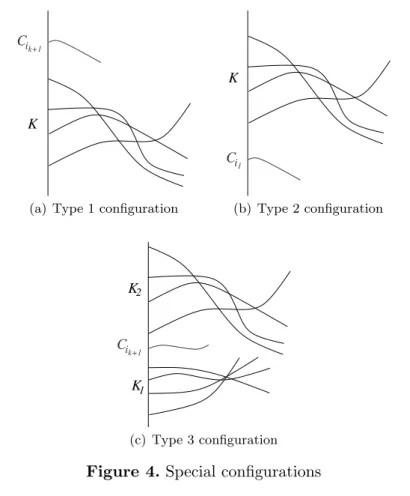
In this section, we will show that if the chromatic number of G(F ) is suffi-ciently high, then certain subconfigurations must exist. We say that the set of curves {Ci1, Ci2, . . . , Cik+1} forms a type 1 configuration, if
1. i1< i2< · · · < ik+1,
2. the set of k curves K = {Ci1, Ci2, . . . , Cik} pairwise intersects,
3. Cik+1 does not intersect any of the curves in K, and
4. x(Cik+1) < x(K). See Figure 4.(a).
Likewise, we say that the set of curves {Ci1, Ci2, . . . , Cik+1} forms a type
2 configuration, if 1. i1< i2< · · · < ik+1,
2. the set of k curves K = {Ci2, Ci3, . . . , Cik+1} pairwise intersects,
3. Ci1 does not intersect any of the curves in K, and
4. x(Ci1) < x(K). See Figure 4.(b).
We say that the set of curves {Ci1, Ci2, . . . , Ci2k+1} forms a type 3
config-uration, if
1. i1< i2< · · · < i2k+1,
2. the set of k curves K1= {Ci1, . . . , Cik} pairwise intersects,
3. the set of k curves K2= {Cik+2, Cik+3, . . . , Ci2k+1} pairwise intersects,
4. Cik+1 does not intersect any of the curves in K1∪ K2, and
5. x(Cik+1) ≤ x(K1∪ K2). See Figure 4.(c).
Note that in a type 3 configuration, a curve in K1 may or may not
inter-sect a curve in K2. The goal of this subsection will be to show that if G(F )
has large chromatic number, then it must contain a type 3 configuration. We start by proving several lemmas.
Lemma 4.3. Let F = {C1, C2, . . . , Cn} be a family of n x-monotone
right-flag curves. Suppose the set of curves K = {Ci1, Ci2, . . . , Cim} pairwise
inter-sect with i1< i2< · · · < im. If there exits a curve Cj such that Cj is disjoint
to all members in K and i1< j < im, then
i C
k+1
K
(a) Type 1 configuration
i C 1 K (b) Type 2 configuration i C k+1 2 1 K K (c) Type 3 configuration Figure 4. Special configurations
Proof. Suppose that x(Cit) < x(Cj) for some t. Without loss of generality,
we can assume i1 < j < it. Since Ci1 and Cit cross and are x-monotone,
this implies that either Ci1 or Cit intersects Cj and therefore we have a
contradiction. A symmetric argument holds if it< j < im.
Lemma 4.4. Let F = {C1, C2, . . . , Cn} be a family of n x-monotone
right-flag curves. Then for any set of t curves Ci1, Ci2, . . . , Cit∈ F where t ≤ 2k, if
χ(F ) > 2β, then either
1. F contains k + 1 pairwise crossing members, or
2. there exists a subset H ⊂ F\{Ci1, Ci2, . . . , Cit}, such that each curve Cj∈ H
is disjoint to all members in {Ci1, Ci2. . . , Cit}, and χ(H) > 2
β− 22λk.
Proof.
For each j ∈ {1, 2, . . . , t}, let Hj⊂ F be the subset of curves that intersect
Cij. If χ(Hj) > 2
crossing members. Therefore, we can assume that χ(Hj) ≤ 2λkfor all 1 ≤ j ≤ t.
Now let H ⊂ F be the subset of curves defined by H = F \ (H1∪ H2∪ · · · ∪ Ht).
Since χ(F ) > 2β, we have
χ(H) > 2β− t2λk ≥ 2β− 22λk,
where the last inequality follows from the fact that log t < log 2k < λk.
Lemma 4.5. Let F = {C1, C2, . . . , Cn} be a family of n x-monotone
right-flag curves. If χ(F ) ≥ 24λk+107, then either
1. F contains k + 1 pairwise crossing members, or 2. F contains a type 1 configuration, or
3. F contains a type 2 configuration.
Proof. Assume that F does not contain k + 1 pairwise crossing members. By Lemma 3.2, for some d ≥ 2, the subset of curves Fd at distance d from curve C1 satisfies
χ(Fd) ≥ χ(F )
2 ≥ 2
4λk+106.
By Lemma 3.1, there exists a subset H1⊂ Fd such that χ(H1) > 2, and
for every pair of curves Ca, Cb∈ H1 that intersect, Fd(a, b) ≥ 24λk+104. Fix
two such curves Ca, Cb∈ H1 and let A be the set of curves in F (a, b) that
intersects either Ca or Cb. By Lemma 4.1, there exists a subset D1⊂ Fd(a, b)
such that each curve Ci∈ D1 is disjoint to Ca, Cb, A, and moreover,
χ(D1) ≥ 24λk+104− 2λk+1− k · 22λk+102 > 24λk+103.
Again by Lemma 3.1, there exists a subset H2⊂ D1 such that χ(H2) > 2λk,
and for each pair of curves Cu, Cv∈ H that intersect, χ(D1(u, v)) ≥ 23λk+102.
Therefore, H2 contains k pairwise crossing curves Ci1, . . . , Cik such that i1<
i2 < · · · < ik. Since χ(D1(i1, i2)) ≥ 23λk+102, by Lemma 4.4, there exists a
subset D2⊂ D(i1, i2) such that every curve Cl∈ D2 is disjoint to the set of
curves {Ci1, . . . , Cik} and
χ(D2) ≥ 23λk+102− 22λk > 23λk+101.
By applying Lemma 3.1 one last time, there exists a subset H3⊂ D2such that
χ(H3) > 2λk, and for every pair of curves Cu, Cv∈ H3 that intersect, we have
χ(D2(u, v)) ≥ 22λk+100. Therefore, H3contains k pairwise intersecting curves
i1 i2 jk Cq jk−1 Cb Ca r r r r 0 1 2 3 (a) Curve Cq i1 i2 jk jk−1 p d−1 C Cq’ Cb Ca r r r r 0 1 2 3 (b) Curve Cq0 Figure 5. Lemma 4.5 22λk+100, by Lemma 4.4, there exists a subset D
3⊂ D2(jk−1, jk) such that
every curve Cl∈ D3is disjoint to the set of curves {Cj1, . . . , Cjk} (and disjoint
to the set of curves {Ci1, Ci2, . . . , Cik}) and
χ(D3) ≥ 22λk+100− 22λk > 22λk+99.
Now we can define a 22λk+1-sequence {r
i}mi=0 of D3 such that m ≥ 4 (recall
the definition of an α-sequence of F from Section 2). That is, we have subsets D3[r0, r1], D3(r1, r2], . . . , D3(rm−1, rm] that satisfies
1. jk−1< r0< r1< · · · < rm< jk, and
2. χ(D3[r0, r1]) = χ(D3(r1, r2]) = · · · = χ(D3(rm−2, rm−1]) = 22λk+1.
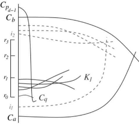
Fix a curve Cq∈ D3(r1, r2]. See Figure 5.(a).
Since Cq∈ D2(r1, r2] ⊂ Fd, there is a path C1, Cp1, Cp2, . . . , Cpd−1, Cq such
that Cpt is at distance t from C1 for 1 ≤ t ≤ d − 1. Let R be the region
enclosed by the y-axis, Ca and Cb. Since Cq lies inside of R, and C1 lies
outside of R, there must be a curve Cpt that intersects either Ca or Cb for
some 1 ≤ t ≤ d − 1. Since Ca, Cb∈ Fd and Cq∈ D1, Cpd−1 must be this curve
and we must have either pd−1< a or pd−1> b. Now the proof splits into two
cases.
Case 1. Suppose pd−1< a. By Lemma 4.3, we have
x(Cq) ≤ x({Cj1, Cj2, . . . , Cjk−1}),
which implies that the set of k curves K = {Cpd−1, Cj1, Cj2, . . . , Cjk−1} are
there exists a curve Cq0∈ D3[r0, r1] such that the curve Cq0 intersects neither
Cpd−1 nor Cq. See Figure 5.(b). By construction of D3[r0, r1], Cq0 does not
intersect any of the curves in the set K ∪ {Cq}. By Lemma 4.3, we have
x(Cq0) ≤ x(Cq) ≤ x(K).
Hence, K ∪ {Cq0} is a type 1 configuration.
Case 2. If pd−1> b, then by a symmetric argument, F contains a type 2
configuration.
Lemma 4.6. Let F = {C1, C2, . . . , Cn} be a family of n x-monotone
right-flag curves. If χ(F ) > 25λk+116, then F contains k + 1 pairwise crossing
members or a type 3 configuration.
Proof. Assume that F does not contain k + 1 pairwise crossing members. By Lemma 3.2, for some d ≥ 2, the subset of curves Fd at distance d from C1 satisfies
χ(Fd) ≥ χ(F ) 2 > 2
5λk+115.
Recall that for each curve Ci∈ Fd, there is a path C1, Cp1, Cp2, . . . , Cpd−1, Ci
such that Cpt is at distance t from C1. Now we define subsets F1, F2⊂ F
d
as follows:
(7)
F1 = {Ci ∈ Fd: there exists a path C1, Cp1, Cp2, . . . , Cpd−1, Ci
with pd−1> i.},
F2 = {Ci ∈ Fd: there exists a path C1, Cp1, Cp2, . . . , Cpd−1, Ci
with pd−1< i.}.
Since F1∪ F2= Fd, either χ(F1) ≥ χ(Fd)/2 or χ(F2) ≥ χ(Fd)/2. Since the
following argument is the same for both cases, we will assume that χ(F1) ≥
χ(Fd)
2 ≥ 2
5λk+114.
By Lemma 3.1, there exists a subset H1⊂ F1 such that χ(H1) > 2, and
for every pair of curves Ca, Cb∈ H1 that intersect, F1(a, b) ≥ 25λk+112. Fix
two such curves Ca, Cb∈ H1 and let A be the set of curves in F (a, b) that
intersects either Caor Cb. By Lemma 4.1, there exists a subset D1⊂ F1(a, b)
such that each curve Ci∈ D1 is disjoint to Ca, Cb, A, and moreover,
χ(D1) ≥ 25λk+112− 2λk+1− k · 22λk+102 > 25λk+111.
Again by Lemma 3.1, there exists a subset H2⊂ D1 such that χ(H2) > 2λk,
Therefore, H2 contains k pairwise crossing members Ci1, Ci2. . . , Cik for i1<
i2 < · · · < ik. Since χ(D1(i1, i2)) ≥ 24λk+110, by Lemma 4.4, there exists a
subset D2⊂ D1(i1, i2) such that
χ(D2) > 24λk+110− 22λk > 24λk+109,
and each curve Cl∈ D2 is disjoint to the set of curves {Ci1, Ci2, . . . , Cik}. Now
we define a 24λk+107-sequence {r
i}mi=0 of D2 such that m ≥ 4. Therefore, we
have subsets
D2[r0, r1], D2(r1, r2], . . . , D2(rm−1, rm]
such that
χ(D2[r0, r1]) = χ(D2(r1, r2]) = 24λk+107.
By Lemma 4.5, we know that D2[r0, r1] contains either a type 1 or type 2
configuration.
Suppose that D2[r0, r1] contains a type 2 configuration {K1, Cq}, where
K1 is the set of k pairwise intersecting curves. See Figure 6.(a). Cq ∈
D2[r0, r1] ⊂ Fd implies that there exists a path C1, Cp1, Cp2, . . . , Cpd−1, Cq
such that pd−1> q. Let R be the region enclosed by the y-axis, Ca and Cb.
Since Cq lies inside of R, and C1 lies outside of R, there must be a curve
Cpt that intersects either Ca or Cb for some 1 ≤ t ≤ d − 1. Since Ca, Cb∈ F
d,
Cpd−1 must be this curve. Moreover, Cq∈ D1 ⊂ F1 implies that pd−1> b.
Since our curves are x-monotone and x(Cq) ≤ x(K1), Cpd−1 intersects all of
the curves in K1. This creates k +1 pairwise crossing members in F and we
have a contradiction. See Figure 6.(b).
i1 r0 r1 r3 r2 Cq K1 Cb Ca i2
(a) Type 2 configuration
i1 r0 r1 r3 r2 Cq K1 Cb d−1 p C Ca i2
(b) k + 1 pairwise crossing curves Figure 6. Lemma 4.6
i1 r0 r1 r3 r2 Cb d−1 p C Cq K1 Ca i2
(a) Type 1 configuration
i1 r0 r1 r3 r2 Cb d−1 p C K1 Cq Ca i2 q’ C (b) Type 3 configuration Figure 7. Lemma 4.6
Therefore, we can assume that D2[r0, r1] contains a type 1 configuration
{K1, Cq} where K1 is the set of k pairwise intersecting curves. See Figure
7.(a). By the same argument as above, there exists a curve Cpd−1 that
in-tersects Cq such that pd−1> b. Hence, K2= {Ci2, Ci3, . . . , Cik, Cpd−1} is a set
of k pairwise intersecting curves. Since χ(D2(r1, r2]) = 24λk+107, Lemma 4.4
implies that there exists a curve Cq0∈ D1(r1, r2] that intersects neither Cq
nor Cpd−1. By construction of D2(r1, r2] and by the definition of a type 1
configuration, Cq0 does not intersect any members in the set {K1, K2, Cq}.
By Lemma 4.3, we have
x(Cq0) ≤ x(Cq) ≤ x(K1∪ K2),
and therefore K1, K2, Cq0 is a type 3 configuration. See Figure 7.(b).
5. Proof of the Theorem 2.1
The proof is by induction on k. The base case k = 2 is trivial. Now suppose that the statement is true up to k. Let F = {C1, C2, . . . , Cn} be a simple
family of n x-monotone right-flag curves, such that χ(F ) > 2(5k+2−121)/4. We will show that F contains k + 1 pairwise crossing members. We define the recursive function λk such that λ2= 1 and
This implies that λk= (5k+1− 121)/4 for all k ≥ 2. Therefore, we have
χ(F ) > 2(5k+2−121)/4= 2λk+1 = 25λk+121.
Just as before, there exists an integer d ≥ 2, such that the set of curves Fd⊂ F at distance d from the curve C
1 satisfies
χ(Fd) ≥ χ(F ) 2 > 2
5λk+120.
Now we can assume that Fddoes not contain k+1 pairwise crossing members, since otherwise we would be done. By Lemma 3.1, there exists a subset H ⊂ Fd such that χ(H) > 2, and for every pair of curves C
a, Cb∈ H that
intersect, Fd(a, b) ≥ 25λk+118. Fix two such curves C
a, Cb∈ H, and let A be
the set of curves in F (a, b) that intersects Ca or Cb. By Lemma 4.1, there
exists a subset D ⊂ Fd(a, b) such that each curve Ci∈ D is disjoint to Ca,
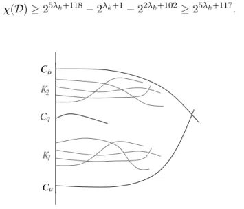
Cb, A, and moreover, χ(D) ≥ 25λk+118− 2λk+1− 22λk+102≥ 25λk+117. Cb 2 K 1 K Cq Ca
Figure 8. Type 3 configuration
By Lemma 4.6, D contains a type 3 configuration {K1, K2, Cq}, where Kt
is a set of k pairwise intersecting curves for t ∈ {1, 2}. See Figure 8. Just as argued in the proof of Lemma 4.6, since Cq∈ D ⊂ Fd, there exists a path
C1, Cp1, Cp2, . . . , Cpd−1, Cq in F such that either pd−1< a or pd−1> b. Since
our curves are x-monotone and x(Cq) ≤ x(K1∪ K2), this implies that either
K1∪Cpd−1 or K2∪Cpd−1 are k +1 pairwise crossing curves. See Figures 9.(a)
Cb 2 K 1 K Cq d−1 p C Ca
(a) K1∪ Cpd−1 are k + 1 pairwise crossing curves Cb 2 K 1 K Cq d−1 p C Ca (b) K2∪ Cpd−1 are k + 1 pairwise crossing curves Figure 9. k + 1 pairwise crossing curves
References
[1] P. K. Agarwal, M. van Kreveld and S. Suri: Label placement by maximum independent set in rectangles, Comput. Geom. Theory Appl. 11 (1998), 209–218. [2] E. Asplund and B. Gr¨unbaum: On a coloring problem, Math. Scand. 8 (1960), 181–
188.
[3] J. P. Burling: On coloring problems of families of prototypes, Ph. D. Thesis, Univ of Colorado, 1965.
[4] P. Erd˝os: Graph theory and probability, Candian J. of Mathematics 11 (1959), 34– 38.
[5] J. Fox and J. Pach: Coloring Kk-free intersection graphs of geometric objects in the plane European Journal of Combinatorics, to appear.
[6] J. Fox, J. Pach and Cs. T´oth: Intersection patterns of curves, J. Lond Math. Soc., 83 (2011), 389–406.
[7] Z. F¨uredi: The maximum number of unit distances in a convex n-gon, J. Comb. Theory, Ser. A 55 (1990), 316–320.
[8] A. Gy´arf´as: On the chromatic number of multiple intervals graphs and overlap graphs, Discrete Math., 55 (1985), 161–166.
[9] A. Gy´arf´as and J. Lehel: Covering and coloring problems for relatives of intervals, Discrete Math. 55 (1985), 167–180.
[10] D. S. Hochbaum and W. Maass: Approximation schemes for covering and packing problems in image processing and VLSI, J. ACM 32 (1985), 130–136.
[11] S. Kim, A. Kostochka and K. Nakprasit: On the chromatic number of intersection graphs of convex sets in the plane, Electr. J. Comb. 11 (2004), 1–12.
[12] A. Kostochka and J. Kratochv´ıl: Covering and coloring polygon-circle graphs, Discrete Mathematics 163 (1997), 299–305.
[13] A. Kostochka and J. Neˇsetˇril: Coloring relatives of intervals on the plane, I: chromatic number versus girth, European Journal of Combinatorics 19 (1998), 103– 110.
[14] A. Kostochka and J. Neˇsetˇril: Coloring relatives of intervals on the plane, II: intervals and rays in two directions, European Journal of Combinatorics 23 (2002), 37–41.
[15] S. McGuinness: On bounding the chromatic number of L-graphs, Discrete Math. 154 (1996), 179–187.
[16] S. McGuinness: Colouring arcwise connected sets in the plane, I, Graphs Combin. 16 (2000), 429–439.
[17] S. McGuinness: Colouring arcwise connected sets in the plane, II, Graphs Combin. 17 (2001), 135–148.
[18] J. Pach and P. Agarwal: Combinatorial Geometry, Wiley Interscience, New York, 1995.
[19] A. Pawlik, J. Kozik, T. Krawczyk, M. Laso´n, P. Micek, W. Trotter and B. Walczak: Triangle-free intersection graphs of line segments with large chromatic number, submitted.
[20] A. Suk: k-quasi-planar graphs, in: Proceedings of the 19th International Symposium on Graph Drawing, 2011, 264–275.
[21] P. Valtr: Graph drawings with no k pairwise crossing edges, in: Proceedings of the 5th International Symposium on Graph Drawing, 1997, 205–218.
[22] D. West: Introduction to Graph Theory, 2nd edition, Prentice-Hall, Upper Saddle River, 2001.
Andrew Suk
Massachusetts Institute of Technology Cambridge