Applications of particle physics to the early universe

Applications of Particle Physics to the Early

Universe

by

Leonardo Senatore

Submitted to the Department of Physics

in partial fulfillment of the requirements for the degree of

Doctor of Philosophy in Physics

at the

MASSACHUSETTS INSTITUTE OF TECHNOLOGY

June 2006

( Massachusetts Institute of Technology 2006. All rights reserved.

Author

...-.

Department of Physics

May 5, 2006

Certified by.

...

Alan Guth

Victor F. Weisskopf Professor of Physics

;ghegis Supqrvisor

Certified

by...

Professor of Physics

Thesis Supervisor

Accepted

by...

...

V

-.' '

.f

.

.

.'. . ""-

'Thoma

' Greytak

Associate Department Head ff Education

ARCHIVES

MASSACHU i i $IIThTNO

OF TECHNOLOGY Al lt. n r

Applications of Particle Physics to the Early Universe

Leonardo Senatore

Submitted to the Department of Physics on May 5, 2006, in partial fulfillment of the

requirements for the degree of Doctor of Philosophy in Physics

Abstract

In this thesis, I show some of the results of my research work in the field at the crossing between Cosmology and Particle Physics. The Cosmology of several models of the Physics Beyond the Standard Model is studied. These range from an inflation-ary model based on the condensation of a ghost-like scalar field, to several models motivated by the possibility that our theory is described by a landscape of vacua, as probably implied by String Theory, which have influence on the theory of Baryogen-esis, of Dark Matter, and of Big Bang Nucleosynthesis. The analysis of the data of the experiment WMAP on the CMB for the search of a non-Gaussian signal is also presented and it results in an upper limit on the amount on non-Gaussianities which is at present the most precise and extended available.

Thesis Supervisor: Alan Guth

Title: Victor F. Weisskopf Professor of Physics Thesis Supervisor: Nima Arkani-Hamed

Acknowledgments

I would like to acknowledge my supervisors, Prof. Alan Guth, from whom I learnt the scientific rigor, and Prof. Nima Arkani-Hamed, whose enthusiasm is always an inspiration; the other professors with whom I had the pleasure to interact with: Prof. Matias Zaldarriaga, Prof. Max Tegmark, and in particular Prof. Paolo Creminelli, with whom I ended up spending a large fraction of my time both at work and out of work; all the many Post-Docs and students who helped me, in particular Alberto Nicolis; and eventually all the friends I have met in the journey which brought me here. Often I was in the need of help, and I have always found someone that, smiling, was happy to give it to me. It is difficult to imagine, being a foreign far from home, if without all these people I would have been able to arrive to this point.

At the end, a special thank must go to my parents and to my girlfriend, who have always been close to me.

Contents

1 Introduction

2 Tilted Ghost Inflation

2.1 Introduction. 2.2 Density Perturbations. 2.3 Negative Tilt. 2.3.1 2-Point Function ... 2.3.2 3-Point Function ... 2.3.3 Observational Constraints 2.4 Positive Tilt ... 2.5 Conclusions ...

3 How heavy can the Fermions in Spli and Extradimensional LSP.

3.1 Introduction.

3.2 Gauge Coupling Unification . . . 3.2.1 Gaugino Mass Unification 3.2.2 Gaugino Mass Condition fro 3.3 Hidden sector LSP and Dark Matt, 3.4 Cosmological Constraints ... 3.5 Gravitino LSP ...

3.5.1 Neutral Higgsino, Neutral A

3.5.2 Photino NLSP ... 14 . . . 14 . . . 16 . . . 18 . . . 18 . . . 21 . . . 27 . . . 29 . . . 33

it Susy be? A study on Gravitino 36 . . . 37 . . . 39 . . . 42 om Anomaly Mediation ... 45 er Abundance . . . .... 48 . . . 51 . . . 56

Vino, and Chargino NLSP ... 58

. . . 61

3.5.3 Bino NLSP. 3.6 Extradimansional LSP ... 3.7 Conclusions ... 3.7.1 Gravitino LSP ... 3.7.2 ExtraDimensional LSP .

... .. 63

4 Hierarchy from Baryogenesis 76 4.1 Introduction . . . ... 77

4.2 Hierarchy from Baryogenesis . . . .... 80

4.2.1 Phase Transition more in detail . ... 85

4.3 Electroweak Baryogenesis . ... 89

4.3.1 CP violation sources ... 91

4.3.2 Diffusion Equations . . . ... 100

4.4 Electric Dipole Moment ... 106

4.5 Comments on Dark Matter and Gauge Coupling Unification ... 111

4.6 Conclusions . . . ... 112

4.7 Appendix: Baryogenesis in the Large Velocity Approximation .... 114

5 Limits on non-Gaussianities from WMAP data 5.1 Introduction. 5.2 A factorizable equilateral shape ... 5.3 Optimal estimator for fNL ... 5.4 Analysis of WMAP 1-year data ... 5.5 Conclusions ... 6 The Minimal Model for Dark Matter and Unification 6.1 Introduction. 6.2 The Model . 6.3 Relic Abundance. 6.3.1 Higgsino Dark Matter. 6.3.2 Bino Dark Matter . 123

...

124

...

127

...

133

...

137

...

144

...

155

...

158

6.4 Direct Detection ... 165

6.5 Electric Dipole Moment ... 166

6.6 Gauge Coupling Unification . . . .. .. 168

6.6.1 Running and matching . . . ... 171

6.7 Conclusion ... 178

6.8 Appendix A: The neutralino mass matrix . ... 179

6.9 Appendix B: Two-Loop Beta Functions for Gauge Couplings ... 180

Chapter 1

Introduction

During my studies towards a PhD in Theoretical Physics, I have focused mainly on the connections between Cosmology and Particle Physics.

In the very last few years, there has been a huge improvement in the field of Obser-vational Cosmology, in particular thanks to the experiments on the cosmic microwave background (CMB) and on large scale structures. The much larger precision of the observational data in comparison with just a few years ago has made it possible to make the connection with the field of Theoretical Physics much stronger. This has occurred at a time in which the field of Particle Physics is experiencing a deficiency of experimental data, so that the indications coming from the observational field of Cosmology have become very important, or even vital. This is particularly true, for example, for the possible Physics associated with the ultra-violet (UV) completion of Einstein's General Relativity (GR), as, for example, String Theory.

Because of this, Cosmology has become both a field where new ideas from Particle Physics can be tested, potentially even verified or ruled out with great confidence, and finally applied in search for a more complete understanding of the early history of the universe, and also a field which, with its observations, can motivate new ideas on the Physics of the fundamental interactions.

Some scientific events which occurred during my years as a graduate student have particularly influenced my work.

Anisotropy Probe (WMAP) experiment on the CMB have greatly improved our knowledge of the current cosmological parameters [1]. These new measurements have gone into the direction of verifying the generic predictions of the presence of a pri-mordial inflationary phase in our universe, even though not yet at the necessary high confidence level to insert inflation in the standard paradigm for the history of the early universe. The first careful study of the non-Gaussian features of the CMB has been of particular importance for my work, as I will highlight later. Further, these new data have shown with high confidence the detection of the presence of a form of energy, called Dark Energy, very similar to the one associated with a cosmological constant, which at present dominates the whole energy of the universe.

This last very unexpected discovery from Cosmology is an example of how cosmo-logical observations can affect the field of Theoretical Physics. In fact, this observation has been of great influence on the development of a new set of ideas in Theoretical Physics which have strongly influenced my work. In fact, the problem of the smallness of the cosmological constant is one of the biggest unsolved problems of present The-oretical Physics, and, until these discoveries, it had been hoped that a UV complete theory of Quantum Gravity, once understood, would have given a solution. However, from the theoretical side, String Theory, which is, up to now, the only viable candi-date for being a UV completion of GR, has shown that there exist consistent solutions with a non-null value of the cosmological constant, and that there could be a huge Landscape of consistent solutions, with different low energy parameters. Therefore, the theoretical possibility that the cosmological constant could be non zero, and that it could have many different values according to the different possible histories of the universe, together with the observational fact that the cosmological constant in our universe appears to be non zero, has led to a revival of a proposal by Weinberg [2] that the environmental, or anthropic, argument that structures should be present in our universe in order for there to be life, could force the value of the cosmological constant to be small. Recently, this argument has then been extended to the possi-bility that also other parameters of the low energy theory might be determined by environmental arguments [3, 4]. For obvious reasons, this general class of ideas is

usually referred to as Landscape motivated, and here I will do the same.

In this thesis, I will illustrate some of the works I did into these directions. I con-sider useful to explain them in the chronological order in which they were developed.

In chapter 2, I will develop a model of inflation where the acceleration of the universe is driven by the ghost condensate [5] . The ghost condensate is a recently proposed mechanism through which the vacuum of a scalar field can be characterized by a constant, not null, speed for the field [6]. The inflationary model based on this has the interesting features of generically predicting a detectable level of non-Gaussianities in the CMB, and of being the first example which shows that it is possible to have an inflationary model where the Hubble rate grows with time. The studies performed in this work have resulted in the publication in the journal Physical Review D of the paper in [7].

In chapter 3, in the context of Split Supersymmetry [3], which is a recently pro-posed supersymmetric model motivated by the Landscape where the scalar super-partners are very heavy, and the higgs mass is finely tuned for environmental reasons, I will study the possibility that the dark matter of the universe is made up of par-ticles which interact only gravitationally, such as the gravitino. This possibility, if realized in nature, would have deep consequences on the possible spectrum of Split Supersymmetry and its possible detection at the next Large Hadron Collider (LHC). I will conclude that observational bounds from Big Bang Nucleosynthesis strongly constrain the possibility that the gravitino is the dark matter in the context of Split Supersimmetry, while other hidden sector candidates are still allowed. The stud-ies performed in this work have resulted in the publication in the journal Physical Review D of the paper in [8].

In chapter 4, I will study a model developed in the context of the Landscape, in which the hierarchy between the Weak scale and the Plank scale is explained in terms of requiring that baryons are generated in our universe through the mechanism of Electroweak Baryogenesis. While the signature of this model at LHC could be

very little, the constraint from baryogenesis implies that the system is expected to show up within next generation experiments on the electron electric dipole moment (EDM). The studies performed in this work have resulted in the publication in the journal Physical Review D of the paper in [9].

In chapter 5, I will show a work in which I performed the analysis of the actual data on the CMB from the WMAP experiment, in search of a signal of non-Gaussianity in the temperature fluctuations. I will improve the analysis done by the WMAP team, and I will extend it to other physically motivated models. At the moment, the limit I will quote on the amplitude of the non-Gaussian signal is the most stringent and complete available. The studies performed in this work have resulted in the publi-cation of the paper in [10], accepted for publipubli-cation by the Journal of Cosmology and Astroparticle Physics in May 2006.

In chapter 6, again inspired by the possibility that there is a Landscape of vacua in the fundamental theory, and that the Higgs particle mass might be finely tuned for environmental reasons, I will study the minimal model beyond the Standard Model that would account for the dark matter in the universe as well as gauge coupling unification. I will find that this minimal model can allow for exceptionally heavy dark matter particles, well beyond the reach of LHC, but that the model should however reveal itself within next generation experiments on the EDM. I will embed the model in a Grand Unified Extradimenesional Theory with an extra dimension in an interval, and I will study in detail its properties. The studies performed in this work has resulted in the publication in the journal Physical Review D of the paper

in [11].

This will conclude a summary of some of the research work I have been doing during these years.

Both the field of Cosmology and of Particle Physics are expecting great results from the very next years.

Improvement of the data from WMAP experiment, as well as the launch of Plank and CMBPol experiments are expected to give us enough data to understand with

confidence the primordial inflationary era of our universe. A detection in the CMB of a tilt in the power spectrum of the scalar perturbations, or of a polarization induced by a background of gravitational waves, or of a non-Gaussian signal would shed light into the early phases of the universe, and therefore also on the Physics at very high energy well beyond what at present is conceivable to reach at particle accelerators. Combined with a definite improvement in the data on the Supernovae, expected in the very near future, these new experiment might shed light also on the great mystery of the present value of the Dark Energy, testing with great accuracy the possibility that it is constituted by a cosmological constant.

The turning on of LHC will probably let us understand if the solution to the hierarchy problem is to be solved in some natural way, as for example with TeV scale Supersymmetry, or if there is evidence of a tuning which points towards the presence of a Landscape.

It is a pleasure to realize that by the next very few years, many of these deep questions might have an answer.

Bibliography

[1] D. N. Spergel et al. [WMAP Collaboration], "First Year Wilkinson Microwave Anisotropy Probe (WMAP) Observations: Determination of Cosmological Pa-rameters," Astrophys. J. Suppl. 148, 175 (2003) [arXiv:astro-ph/0302209]. [2] S. Weinberg, "Anthropic Bound On The Cosmological Constant," Phys. Rev.

Lett. 59 (1987) 2607.

[3] N. Arkani-Hamed and S. Dimopoulos, "Supersymmetric unification without low energy supersymmetry and signatures for fine-tuning at the LHC," JHEP 0506, 073 (2005) [arXiv:hep-th/0405159].

[4] N. Arkani-Hamed, S. Dimopoulos and S. Kachru, "Predictive landscapes and new physics at a TeV," arXiv:hep-th/0501082.

[5] N. Arkani-Hamed, P. Creminelli, S. Mukohyama and M. Zaldarriaga, "Ghost inflation," JCAP 0404, 001 (2004) [arXiv:hep-th/0312100].

[6] N. Arkani-Hamed, H. C. Cheng, M. A. Luty and S. Mukohyama, "Ghost con-densation and a consistent infrared modification of gravity," JHEP 0405, 074

(2004) [arXiv:hep-th/0312099].

[7] L. Senatore, "Tilted ghost inflation," Phys. Rev. D 71, 043512 (2005) [arXiv:astro-ph/0406187].

[8] L. Senatore, "How heavy can the fermions in split SUSY be? A study on grav-itino and extradimensional LSP," Phys. Rev. D 71, 103510 (2005) [arXiv:hep-ph/0412103].

[9] L. Senatore, "Hierarchy from baryogenesis," Phys. Rev. D 73, 043513 (2006) [arXiv:hep-ph/0507257].

[10] P. Creminelli, A. Nicolis, L. Senatore, M. Tegmark and M. Zaldarriaga, "Limits on non-Gaussianities from WMAP data," arXiv:astro-ph/0509029.

[11] R. Mahbubani and L. Senatore, "The minimal model for dark matter and unifi-cation," Phys. Rev. D 73, 043510 (2006) [arXiv:hep-ph/0510064].

Chapter 2

Tilted Ghost Inflation

In a ghost inflationary scenario, we study the observational consequences of a tilt in the potential of the ghost condensate. We show how the presence of a tilt tends to

make contact between the natural predictions of ghost inflation and the ones of slow roll inflation. In the case of positive tilt, we are able to build an inflationary model

in which the Hubble constant H is growing with time. We compute the amplitude and the tilt of the 2-point function, as well as the 3-point function, for both the cases of positive and negative tilt. We find that a good fraction of the parameter space of the model is within experimental reach.

2.1 Introduction

Inflation is a very attractive paradigm for the early stage of the universe, being able to solve the flatness, horizon, monopoles problems, and providing a mechanism to generate the metric perturbations that we see today in the CMB [1].

Recently, ghost inflation has been proposed as a new way for producing an epoch of inflation, through a mechanism different from that of slow roll inflation [2, 3]. It can be thought of as arising from a derivatively coupled ghost scalar field which

condenses in a background where it has a non zero velocity:

(X) = 2 (q) = MM2t (2.1)

where we take M2 to be positive.

Unlike other scalar fields, the velocity (X) does not redshift to zero as the universe expands, but it stays constant, and indeed the energy momentum tensor is identical of that of a cosmological constant. However, the ghost condensate is a physical fluid, and so, it has physical fluctuations which can be defined as:

= M2t + 7r (2.2)

The ghost condensate then gives an alternative way of realizing De Sitter phases in the universe. The symmetries of the theory allow us to construct a systematic

and reliable effective Lagrangian for 7r and gravity at energies lower than the ghost cut-off M. Neglecting the interactions with gravity, around flat space, the effective Lagrangian for r has the form:

S d4X*2 - a (V27r)2 2i *(V7r)2 + (2.3)

2 21~2 2M2

where a and 3 are order one coefficients. In [2], it was shown that, in order for the ghost condensate to be able to implement inflation, the shift symmetry of the ghost field p had to be broken. This could be realized adding a potential to the ghost. The observational consequences of the theory were no tilt in the power spectrum, a relevant amount of non gaussianities, and the absence of gravitational waves. The non gaussianities appeared to be the aspect closest to a possible detection by experiments such as WMAP. Also the shape of the 3-point function of the curvature perturbation C was different from the one predicted in standard inflation. In the same paper [2], the authors studied the possibility of adding a small tilt to the ghost potential, and they did some order of magnitude estimate of the consequences in the case the potential decreases while X increases.

In this chapter, we perform a more precise analysis of the observational conse-quences of a ghost inflation with a tilt in the potential. We study the 2-point and 3-point functions. In particular, we also imagine that the potential is tilted in such a way that actually the potential increases as the value of X increases with time. This

configuration still allows inflation, since the main contribution to the motion of the ghost comes from the condensation of the ghost, which is only slightly affected by the presence of a small tilt in the potential. This provides an inflationary model in which H is growing with time. We study the 2-point and 3-point function also in this case.

The chapter is organized as follows. In section 2.2, we introduce the concept of the tilt in the ghost potential; in section 2.3 we study the case of negative tilt, we compute the 2-point and 3-point functions, and we determine the region of the parameter space which is not ruled out by observations; in section 2.4 we do the same as we did in section 2.3 for the case of positive tilt; in section 2.5 we summarize our conclusions.

2.2 Density Perturbations

In an inflationary scenario, we are interested in the quantum fluctuations of the r field, which, out of the horizon, become classical fluctuations. In [3], it was shown that, in the case of ghost inflation, in longitudinal gauge, the gravitational potential

1I decays to zero out of the horizon. So, the Bardeen variable is simply:

H

H=

-- - (2.4)

and is constant on superhorizon scales. It was also shown that the presence of a ghost condensate modifies gravity on a time scale r -1_{, with F M}3_{/Mpl, and on a length} scale m-l1, with m - M2/Mpl. The fact that these two scales are different is not a surprise since the ghost condensate breaks Lorentz symmetry.

Hubble horizon, we have to impose < Ho, which implies that gravity is not modified during inflation:

r

<<

m < H

(2.5)

This is equivalent to the decoupling limit Mpl --+ o, keeping H fixed, which implies

that we can study the Lagrangian for r neglecting the metric perturbations.

Now, let us consider the case in which we have a tilt in the potential. Then, the zero mode equation for r becomes:

+ 3H + V' = 0

(2.6)

which leads to the solution:

V'

r=

3H

(2.7)

We see that this is equivalent to changing the velocity of the ghost field.

In order for the effective field theory to be valid, we need that the velocity of 7r to be much smaller than M2, so, in agreement with [2], we define the parameter:

V' 62 =-3HM 2 for V' < 0 (2.8) 3HM2 V' 62 = +

for V' > 0

to be 62 < 1. We perform the analysis for small tilt, and so at first order in 62. At this point, it is useful to write the 0-0 component of the stress energy tensor, for the model of [3]:

To = -M

_{P(X) + 2M}

_P'(X)q

_{+ V(0)}

_(2.9)

where X = 09,Oq50u. The authors show that the field, with no tilted potential, is attracted to the minimum of the function P(X), such that, P(Xmi,) = M2. So,

adding a tilt to the potential can be seen as shifting the ghost field away from the minimum of P(X).

for both the cases of a positive tilt and a negative tilt.

2.3 Negative Tilt

Let us analyze the case V' < 0.

2.3.1 2-Point Function

To calculate the spectrum of the 7r fluctuations, we quantize the field as usual:

rk(t) = Wk(t)ak + W (t)at k

(2.10)

The dispersion relation for Wk is:

k4

W

2 = a-

+

j2k

(2.11)

k M2

±

(2.11)

Note, as in [3], that the sign of p is the same as the sign of < X >= M2. In all this

chapter we shall restrict to P > 0, and so the sign of 3 is fixed.

We see that the tilt introduces a piece proportional to k2 _{in the dispersion relation.} This is a sign that the role of the tilt is to transform ghost inflation to the standard slow roll inflation. In fact, w2 _{- k}2_{is the usual dispersion relation for a light field.}

Defining Wk(t) = uk(t)/a, and going to conformal time dr = dt/a, we get the

following equation of motion:

, k4H2 72 2

up + (/62_k2 _{+ a}

_kH

)u k= 0 (2.12)

If we were able to solve this differential equation, than we could deduce the power spectrum. But, unfortunately, we are not able to find an exact analytical solution. Anyway, from (2.12), we can identify two regimes: one in which the term k4 dominates at freezing out, w - H, and one in which it is the term in - k2 that

shape of the wavefunction comes from the time around horizon crossing. So, in order for the tilt to leave a signature on the wavefunction, we need it to dominate before freezing out.There will be an intermediate regime in which both the terms in k2 _and k4 will be important around horizon crossing, but we decide not to analyze that case as not too much relevant to our discussion. So, we restrict to:

a1/2 H

62 > >2 _ (2.13)

where cr stays for crossing. In that case, the term in k2 dominates before freezing out, and we can approximate the differential equation (2.12) to:

"2

2

Uk

+ (k

_-

_{)uk =}

₀

_(2.14)

Solving with the usual vacuum initial condition, we get:

e-i0

i

Wk =-H7 /2 (1-

)

(2.15)

which leads to the power spectrum:

k3 _H2 P= 2 Iwk( 0)12 = (2.16) Wk (q2 4' 2/33/263 and, using = 7T, H4 PC = 47r2o3/253M4 (2.17)

This is the same result as in slow roll inflation, replacing k with k. Notice that, on the contrary with respect to standard slow roll inflation, the denominator is not suppressed by slow roll parameters, but by the 62 term.

The tilt is given by: dln(P¢)_dln(k) 2M2V' = +

HV

dln(H)

+

4M4

(1- 2P"M8))

where k = -r7/25 is the momenta at freezing out, and where P and its derivatives are evaluated at Xmin.

Notice the appearance of the term - , which can easily be the dominant piece. Please remind that, anyway, this is valid only for 62 > 6c,. Notice also that, for the effective field theory to be valid, we need:

V'

3H

so, Mvi < M . This last piece is in general << 1 if the ghost condensate is present

today. In order to get an estimate of the deviation from scale invariance, we can see that the larger contribution comes from the piece in - vH2. From the validity of the effective field theory, we get:

62M2H IV'I IV"/A) = I V"I(M 2/IH)Ne = V"l < 62

Ne (2.20)

where Ne is the number of e-foldings to the end of inflation. So, we deduce that the deviation of the tilt can be as large as:

Ins- <N

- Ne (2.21)

2.3.2 3-Point Function

Let us come to the computation of the three point function. The leading interaction term (or the least irrelevant one), is given by [2]:

eHt

Lint = -,3 2M2 (*(V702) (2.22)

Using the formula in [4]:

< ,k(t)l(t)7(t) >=-

i

d3xHt(t')]

we get [2]:

2 (27r35( ki)

<7rkl7rk27rk3 >= M2(2)6( k) (2.24) wl(O)w2(O)w3(O)((k2.k3)I(1, 2, 3) + cyclic + c.c)

where cyclic stays for cyclic permutations of the k's, and where

f0 1

I(1,2,3) =

1

and the integration is performed with the prescription that the oscillating functions inside the horizon become exponentially decreasing as --+ -oo.

We can do the approximation of performing the integral with the wave function (2.15). In fact, the typical behavior of the wavefunction will be to oscillate inside the horizon, and to be constant outside of it. Since we are performing the integration on a path which exponentially suppresses the wavefunction when it oscillates, and since in the integrand there is a time derivative which suppresses the contribution when a wavefunction is constant, we see that the main contribution to the three point function comes from when the wavefunctions are around freezing out. Since, in that case, we are guaranteed that the term in k2 dominates, then we can reliably approximate the

wavefunctions in the integrand with those in (2.15). Using that ( = - H7r,we get: H8~~~~~~

H8

< (k(k 2,k3 >= (27r)363(Z ki) 4 36sM (2.26) k3 i~=~l k (k l2( 3) ((k2+ k3)kt + k2+ 2k3k2) + cyclic)

where ki = ki . Let us define

F(k, k2, k3) = 3 3 (k(k 2.k3) ((k2 + k3)kt + kt2 + 2k3k2) + cyclic) (2.27)

which, apart for the function, holds the k dependence of the 3-point function. The obtained result agrees with the order of magnitude estimates given in [2]:

<__3_> 1 H 1 1 H

(< ¢3

1_(H)

>)

I()/

-()2

(2.28)

(< (2 >)3/2 68 M (1(H)2)3/2 67/2 (M (2

The total amount of non gaussianities is decreasing with the tilt. This is in agreement with the fact that the tilt makes the ghost inflation model closer to slow roll inflation, where, usually, the total amount of non gaussianities is too low to be detectable.

The 3-point function we obtained can be better understood if we do the following observation. This function is made up of the sum of three terms, each one obtained on cyclic permutations of the k's. Each of these terms can be split into a part which is typical of the interaction and of scale invariance, and the rest which is due to the wave function. For the first cyclic term, we have:

Interaction (k2.k3) (2.29)

while, the rest, which I will call wave function, is:

((k2 + k3)kt + k + 2k2k3)

Wavefunction

The interaction part appears unmodified also in the untilted ghost inflation case. While the wave function part is characteristic of the wavefunction, and changes in

the two cases.

Our 3-point function can be approximately considered as a function of only two in-dependent variables. The delta function, in fact, eliminates one of the three momenta, imposing the vectorial sum of the three momenta to form a closed triangle. Because of the symmetry of the De Sitter universe, the 3-point function is scale invariant, and so we can choose [ki[ = 1. Using rotation invariance, we can choose k1 = 1, and

impose k₂ to lie in the 61, 62 plane. So, we have finally reduced the 3-point function from being a function of 3 vectors, to be a function of 2 variables. From this, we can choose to plot the 3-point function in terms of xi - ki, i = 1, 2. The result is shown in fig.2-1. Note that we chose to plot the three point function with a measure equal to x2x2. The reason for this is that this results in being the natural measure in the case we wish to represent the ratio between the signal associated to the 3-point function with respect to the signal associated to the 2-point function [5]. Because of the triangular inequality, which implies _{3 <} 1 - x2, and in order to avoid to double

represent the same momenta configuration, we set to zero the three point function outside the triangular region: 1 - x2 _ 3 < x2. In order to stress the difference

with the case of standard ghost inflation, we plot in fig.2-2 the correspondent 3-point function for the case of ghost inflation without tilt. Note that, even though the two shapes are quite similar, the 3-point function of ghost inflation without tilt changes signs as a function of the k's, while the 3-point function in the tilted case has constant sign.

An important observation is that, in the limit as 3 -- 0 and x2 - 1, which

corresponds to the limit of very long and thin triangles, we have that the 3 point function goes to zero as 1 . This is expected, and in contrast with the usual slow

roll inflation result - . The reason for this is the same as the one which creates 3

the same kind of behavior in the ghost inflation without tilt [2]. The limit of x3 --* 0

corresponds to the physical situation in which the mode k3 exits from the horizon, freezes out much before the other two, and acts as a sort of background. In this limit, let us imagine a spatial derivative acting on 7r3, which is the background in

1

0.8

Figure 2-1: Plot of the function F(l, X2, x3)x~x5 for the tilted ghost inflation 3-point function. The function has been normalized to have value 1 for the equilateral config-uration X2 = X3 = 1, and it has been set to zero outside of the region 1 - X2 :SX3 :SX2

1

0.8

0.5 F(x2,x3)

o

Figure 2-2: Plot of the similarly defined function F(l, X2, x3)x~x5 for the standard ghost inflation 3-point function. The function has been normalized to have value 1 for the equilateral configuration X2 = X3 = 1, and it has been set to zero outside of the region 1 - X2 :SX3 :SX2 [5]

on the background wave, and, at linear order, will be proportional to 8(Tr3. The variation of the 2-point function along the 1r3 wave is averaged to zero in calculating

the 3-point function < 7rk 7rk2irk3 >, because the spatial average < 7r3 i7r3 > vanishes. So, we are forced to go to the second order, and we therefore expect to receive a factor of k, which accounts for the difference with the standard slow roll inflation case. In the model of ghost inflation, the interaction is given by derivative terms, which favors the correlation of modes freezing roughly at the same time, while the correlation is suppressed for modes of very different wavelength. The same situation occurs in standard slow roll inflation when we study non-gaussianities generated by higher derivative terms [6].

The result is in fact very similar to the one found in [6]. In that case, in fact, the interaction term could be represented as:

Lint 2(_,2 + e-2Ht(Oip)2) (2.31)

where one of the time derivative fields is contracted with the classical solution. This interaction gives rise to a 3-point function, which can be recast as:

<

k(k

(k

>a

( (ki

)) ((k

+ k

)kt + k

+

2k

k

) + cyclic)

+ (2.32)

12

H f(ka)ka(k + + k3)

We can easily see that the first part has the same k dependence as our tilted ghost inflation. That part is in fact due to the interaction with spatial derivative acting, and it is equal to our interaction. The integrand in the formula for the 3-point function is also evaluated with the same wave functions, so, it gives necessarily the same result as in our case. The other term is due instead to the term with three time derivatives acting. This term is not present in our model because of the spontaneous breaking of Lorentz symmetry, which makes that term more irrelevant that the one with spatial derivatives, as it is explained in [2]. This similarity could have been expected, because, adding a tilt to the ghost potential, we are converging towards standard slow roll inflation. Besides, since we have a shift symmetry for the ghost field, the interaction term which will generate the non gaussianities will be a higher

derivative term, as in [6].

We can give a more quantitative estimate of the similarity in the shape between our three point function and the three point functions which appear in other models. Following [5], we can define the cosine between two three point functions F1(k1, k2, k3),

F2(kl, k2, k3), as:

cos(Fi, F2) (F.

F

F2)1/

(2.33)

where the scalar product is defined as:

Fl(kl, k2, k3) .F₂(k, k₂, k₃) d ₂ dx2 dx F(1,x₂,x₃)F₂(1,x₂,X₃) (2.34)

/2

-x2

where, as before, xi = k. The result is that the cosine between ghost inflation with tilt and ghost inflation without tilt is approximately 0.96, while the cosine with the distribution from slow roll inflation with higher derivatives is practically one. This means that a distinction between ghost inflation with tilt and slow roll inflation with higher derivative terms , just from the analysis of the shape of the 3-point function, sounds very difficult. This is not the case for distinguishing from these two models and ghost inflation without tilt.

Finally, we would like to make contact with the work in [7], on the Dirac-Born-Infeld (DBI) inflation. The leading interaction term in DBI inflation is, in fact, of the same kind as the one in (2.31), with the only difference being the fact that the relative normalization between the term with time derivatives acting and the one with space derivatives acting is weighted by a factor 2 = (1 - v2)-1, where v, is

the gravity-side proper velocity of the brane whose position is the Inflaton. This relative different normalization between the two terms is in reality only apparent, since it is cancelled by the fact that the dispersion relation is w k. This implies the the relative magnitude of the term with space derivatives acting, and the one of time derivatives acting are the same, making the shape of the 3-point function in DBI inflation exactly equal to the one in slow roll inflation with higher derivative couplings, as found in [6].

2.3.3 Observational Constraints

We are finally able to find the observational constraints that the negative tilt in the ghost inflation potential implies.

In order to match with COBE:

1

H

PC = 47r233/2 )43M (4.8 10-5)2 = 0.018l83/ 63/4 (2.35)

From this, we can get a condition for the visibility of the tilt. Remembering that

62 - al/2 ( ), we get that, in order for 6 to be visible:

_3 Mh

208

1/263/4

=4/5

62 62 = 0.018 _/~5/8 5/8 62 > 2ibility = 0.0016 ₁₃ (2.36) In the analysis of the data (see for example [8]), it is usually assumed that the non-gaussianities come from a field redefinition:

3 2

(

=

-

5fNL(C-

<

>)

(2.37)

where Cg is gaussian. This pattern of non-gaussianity, which is local in real space, is characteristic of models in which the non-linearities develop outside the horizon. This happens for all models in which the fluctuations of an additional light field, different from the inflaton, contribute to the curvature perturbations we observe. In this case the non linearities come from the evolution of this field into density perturbations. Both these sources of non-linearity give non-gaussianity of the form (2.37) because they occur outside the horizon. In the data analysis, (2.37) is taken as an ansatz, and limits are therefore imposed on the scalar variable fNL. The angular dependence of the 3-point function in momentum space implied by (2.37) is given by:

< (klk2k3 > = (27r)363( ki)(2W)4(--fNL PR) Hi k (2.38)

In our case, the angular distribution is much more complicated than in the previous expression, so, the comparison is not straightforward. In fact, the cosine between the

two distributions is -0.1. We can nevertheless compare the two distributions (2.27) and (2.37) for an equilateral configuration, and define in this way an "effective" fNL

for kl = k2 = k3. Using COBE normalization, we get:

0.29

fNL

=

(2.39)

The present limit on non-gaussianity parameter from the WMAP collaboration [8] gives:

-58 < fNL < 138 at 95% C.L. (2.40) and it implies:

62 > 0.005 (2.41)

which is larger than 52ivility (which nevertheless depends on the coupling constants a,O0.

Since for 62 >> usiibility we do see the effect of the tilt, we conclude that there is

a minimum constraint on the tilt: 62 > 0.005.

In reality, since the shape of our 3-point function is very different from the one which is represented by fNL, it is possible that an analysis done specifically for this

shape of non-gaussianities may lead to an enlargement of the experimental boundaries. As it is shown in [5], an enlargement of a factor 5-6 can be expected. This would lead to a boundary on 62 of the order 62 > 0.001, which is still in the region of interest for

the tilt.

Most important, we can see that future improved measurements of Non Gaus-sianity in CMB will immediately constraint or verify an important fraction of the parameter space of this model.

Finally, we remind that the tilt can be quite different from the scale invariant result of standard ghost inflation:

]n,

-1< -1 (2.42)

2.4 Positive Tilt

In this section, we study the possibility that the tilt in the potential of the ghost is positive, V' > 0. This is quite an unusual condition, if we think to the case of the slow roll inflation. In this case, in fact, the value of H is actually increasing with time. This possibility is allowed by the fact that, on the contrary with respect to what occurs in the slow roll inflation, the motion of the field is not due to an usual potential term, but is due to a spontaneous symmetry breaking of time diffeomorphism, which gives a VEV to the velocity of the field. So, if the tilt in the potential is small enough, we expect to be no big deviance from the ordinary motion of the ghost field, as we already saw in section one.

In reality, there is an important difference with respect to the case of negative tilt: a positive tilt introduces a wrong sign kinetic energy term for r. The dispersion relation, in fact, becomes:

W2 = - p 2_k2 _(2.43)

The k2 term is instable. The situation is not so bad as it may appear, and the reason is the fact that we will consider a De Sitter universe. In fact, deep in the ultraviolet the term in k4 is going to dominate, giving a stable vacuum well inside the horizon. As momenta are redshifted, the instable term will tend to dominate. However, there is another scale entering the game, which is the freeze out scale w(k) - H. When this occurs, the evolution of the system is freezed out, and so the presence of the instable term is forgotten.

So, there are two possible situations, which resemble the ones we met for the negative tilt. The first is that the term in k2_{begins to dominate after freezing out. In} this situation we would not see the effect of the tilt in the wave function. The second case is when there is a phase between the ultraviolet and the freezing out in which the term in k2 dominates. In this case, there will be an instable phase, which will make the wave function grow exponentially, until the freezing out time, when this growing will be stopped. We shall explore the phase space allowed for this scenario,

which occurs for

a1/ 2_H

3262 > r=

a:/ H

and we restrict to it.

Before actually beginning the computation, it is worth to make an observation. All the computation we are going to do could be in principle be obtained from the case of positive tilt, just doing the transformation 62 _- -62 in all the results we

obtained in the former section. Unfortunately, we can not do this. In fact, in the former case, we imposed that the term in k2 dominates at freezing out, and then solved the wave equation with the initial ultraviolet vacua defined by the term in k2, and not by the one in k4, as, because of adiabaticity, the field remains in the vacua well inside the horizon. On the other hand, in our present case, the term in k2 does not define a stable vacua inside the horizon, so, the proper initial vacua is given by the term in k4 which dominates well inside the horizon. This leads us to solve the full differential equation:

k4H2 72 2

u" + (_

2k2 +

2

=

(2.45)

Since we are not able to find an analytical solution, we address the problem with the semiclassical WKB approximation. The equation we have is a Schrodinger like eigenvalue equation, and the effective potential is:

k4H2 2 2

V = p2k

_{_ a}

_{+ -}

_(2.46)

we have the two semiclassical regions:

for << r7o, the potential can be approximated to:

4 H2r

_(2.48)

while, for > r70:

V= d,32 k2+ 2 (2.49)

772

The semiclassical approximation tells us that the solution, in these regions, is given by: for r << 770: U (p( Al ei fcr p(')d' (2.50) while, for 7r > r70: U (p e-)crP(7)d7' (2.51) where P(77) = (IV(77))1 /2

The semiclassical approximation fails for r7 ro. In that case, one can match the two solution using a standard linear approximation for the potential, and gets A2=

Al e - i 7r/4 [9]. It is easy to see that the semiclassical approximation is valid when

62 62.

Let us determine our initial wave function. In the far past, we know that the solution is the one of standard ghost inflation [2]:

7r12 1 r(1) H k2a

-U=( (-)1/2( 77

)1/2H()

r2)

(2.52)

We can put this solution, for the remote past, in the semiclassical form, to get:

U

= 1 /e e (8+H e 2M 77 (2.53)

(2--k (-77))1/2

So, using our relationship between Al and A2, we get, for r > ro, the following wave function for the ghost field:

1 i _ 7 2He-") H (2.54)

w = u/a 2/2 1/2ei(- * 2H e aH (Hrek" + e-kr/)

(2.54)

Notice that this is exactly the same wave function we would get if we just rotated 5 - i in the solutions we found in the negative tilt case. But the normalization

would be very different, in particular missing the exponential factor, which can be large. It is precisely this exponential factor that reflects the phase of instability in the evolution of the wave function.

From this observation, the results for the 2-point ant 3-point functions are imme-diately deduced from the case of negative tilt, paying attention to the factors coming from the different normalization constants in the wave function.

So, we get:

2162 M 1 e al H

4P 13/2H (H 4 (2.55)

Notice the exponential dependence on a, 3, HIM, and 2.

The tilt gets modified, but the dominating term 1-' is not modified:

n-1 = V2M 2 + _{27r3 62}

_M

n=V'(HV

a H2M

V"/ 1 2 4M 4

M

(- + +(1 - 2P ) + 3H 3M2 (2 - 4P"M 8))

For the three point function, we get:

H8

< kl(k2(k3 >= (27r)363(Z ki) 433a8M8 (2.57)

1 (,62(,Z262

k3 2k3 (kl2(.k3) ((k2 + k3)kt + kt + 2k3k2) + cyclic) e6 H

which has the same k's dependence as in the former case of negative tilt. Estimating the fNL as in the former case, we get:

0.29 6M

fNL - 6 2 e aH (2.58)

Notice again the exponential dependence.

Combining the constraints from the 2-point and 3-point functions, it is easy to see that a relevant fraction of the parameter space is already ruled out. Anyway, because of the exponential dependence on the parameters 62,- , and the coupling constants a, and

3,

configurations that are still allowed.

2.5 Conclusions

We have presented a detailed analysis of the consequences of adding a small tilt to the potential of ghost inflation.

In the case of negative tilt, we see that the model represent an hybrid between ghost inflation and slow roll inflation. When the tilt is big enough to leave some sig-nature, we see that there are some important observable differences with the original case of ghost inflation. In particular, the tilt of the 2-point function of ( is no more exactly scale invariant n, = 1, which was a strong prediction of ghost inflation. The 3-point function is different in shape, and is closer to the one due to higher deriva-tive terms in slow roll inflation. Its total magnitude tends to decrease as the tilt increases. It must be underlined that the size of these effects for a relevant fraction of the parameter space is well within experimental reach.

In the case of a positive tilt to the potential, thanks to the freezing out mecha-nism, we are able to make sense of a theory with a wrong sign kinetic term for the fluctuations around the condensate, which would lead to an apparent instability. Con-sequently, we are able to construct an interesting example of an inflationary model in which H is actually increasing with time. Even though a part of the parameter space is already excluded, the model is not completely ruled out, and experiments such as WMAP and Plank will be able to further constraint the model.

Bibliography

[1] A. H. Guth, "The Inflationary Universe: A Possible Solution To The Horizon And Flatness Problems," Phys. Rev. D 23 (1981) 347. A. D. Linde, "A New Inflationary Universe Scenario: A Possible Solution Of The Horizon, Flatness, Homogeneity, Isotropy And Primordial Monopole Problems," Phys. Lett. B 108 (1982) 389. J. M. Bardeen, P. J. Steinhardt and M. S. Turner, "Spontaneous Creation Of Almost Scale - Free Density Perturbations In An Inflationary Universe," Phys. Rev. D 28 (1983) 679.

[2] N. Arkani-Hamed, P. Creminelli, S. Mukohyama and M. Zaldarriaga, "Ghost in-flation," JCAP 0404 (2004) 001 [arXiv:hep-th/0312100].

[3] N. Arkani-Hamed, H. C. Cheng, M. A. Luty and S. Mukohyama, "Ghost conden-sation and a consistent infrared modification of gravity," arXiv:hep-th/0312099. [4] J. Maldacena, "Non-Gaussian features of primordial fluctuations in single field

inflationary models," JHEP 0305 (2003) 013 [arXiv:astro-ph/0210603]. See also V.Acquaviva, N.Bartolo, S.Matarrese and A.Riotto,"Second-order cosmological perturbations from inflation", Nucl.Phyis. B 667, 119 (2003) [astro-ph/0207295] [5] D. Babich, P. Creminelli and M. Zaldarriaga, "The shape of non-Gaussianities,"

arXiv:astro-ph/0405356.

[6] P. Creminelli, On non-gaussianities in single-field inflation, JCAP 0310 (2003) 003 [arXiv:astro-ph/0306122].

[7] M. Alishahiha, E. Silverstein and D. Tong, "DBI in the sky," arXiv:hep-th/0404084.

[8] E. Komatsu et al., "First Year Wilkinson Microwave Anisotropy Probe (WMAP) Observations: Tests of Gaussianity," Astrophys. J. Suppl. 148 (2003) 119 [arXiv:astro-ph/0302223].

[9] See for example: Ladau, Lifshitz, Quantum Machanics, Vol.III, Butterworth Heinemann ed. 2000.

Chapter 3

How heavy can the Fermions in

Split Susy be? A study on

Gravitino and Extradimensional

LSP.

In recently introduced Split Susy theories, in which the scale of Susy breaking is very high, the requirement that the relic abundance of the Lightest SuperPartner

(LSP) provides the Dark Matter of the Universe leads to the prediction of fermionic superpartners around the weak scale. This is no longer obviously the case if the LSP is a hidden sector field, such as a Gravitino or an other hidden sector fermion, so, it is interesting to study this scenario. We consider the case in which the Next-Lightest SuperPartner (NLSP) freezes out with its thermal relic abundance, and then it decays to the LSP. We use the constraints from BBN and CMB, together with the requirement of attaining Gauge Coupling Unification and that the LSP abundance provides the Dark Matter of the Universe, to infer the allowed superpartner spectrum. As very good news for a possible detaction of Split Susy at LHC, we find that if the Gravitino is the LSP, than the only allowed NLSP has to be very purely photino like. In this case, a photino from 700 GeV to 5 TeV is allowed, which is difficult to test

at LHC. We also study the case where the LSP is given by a light fermion in the hidden sector which is naturally present in Susy breaking in Extra Dimensions. We find that, in this case, a generic NLSP is allowed to be in the range 1-20 TeV, while a Bino NLSP can be as light as tens of GeV.

3.1 Introduction

Two are the main reasons which lead to the introduction of Low Energy Supersymme-try for the physics beyond the Standard Model: a solution of the hierarchy problem, and gauge coupling unification.

The problem of the cosmological constant is usually neglected in the general treat-ment of beyond the Standard Model physics, justifying this with the assumption that its solution must come from a quantum theory of gravity. However, recently [1], in the light of the landscape picture developed by a new understanding of string theory, it has been noted that, if the cosmological constant problem is solved just by a choice of a particular vacua with the right amount of cosmological constant, the statistical weight of such a fine tuning may dominate the fine tuning necessary to keep the Higgs light. Therefore, it is in this sense reasonable to expect that the vacuum which solves the cosmological constant problem solves also the hierarchy problem.

As a consequence of this, the necessity of having Susy at low energy disappears, and Susy can be broken at much higher scales (106 - 109 GeV).

However, there is another important prediction of Low Energy Susy which we do not want to give up, and this is gauge coupling unification. Nevertheless, gauge coupling unification with the same precision as with the usual Minimal Supersym-metric Standard Model (MSSM) can be achieved also in the case in which Susy is broken at high scales. An example of this is the theories called Split Susy [1, 2] where there is an hierarchy between the scalar supersymmetric partners of Standard Model (SM) particles (squarks, sleptons, and so on) and the fermionic superpartners of SM particles (Gaugino, Higgsino), according to which, the scalars can be very heavy at

an intermediate scale of the order of 109 GeV, while the fermions can be around the weak scale. The existence for this hierarchy can be justified by requiring that the chiral symmetry protects the mass of the fermions partners.

While the chiral symmetry justifies the existence of light fermions, it can not fix the mass of the fermionic partners precisely at the weak scale. As a consequence, this theory tends to make improbable the possibility of finding Susy at LHC, because in principle there could be no particles at precisely 1 TeV. In this chapter, for Split Susy, we do a study at one-loop level of the range of masses allowed by gauge coupling unification, finding that these can vary in a range that approximately goes up to 20 TeV. A possible way out from this depressing scenario comes from realizing that cosmological observations indicate the existence of Dark Matter (DM) in the universe. The standard paradigm is that the Dark Matter should be constituted by stable weakly interacting particles which are thermal relics from the initial times of the universe. The Lightest Supersymmetric Partner (LSP) in the case of conserved R-parity is stable, and, if it is weakly interacting, such as the Neutralino, it provides a perfect candidate for the DM. In particular, an actual calculation shows that in order for the LSP to provide all the DM of the universe, its mass should be very close to the TeV scale. This is the very good news for LHC we were looking for. Just to stress this result, it is the requirement the the DM is given by weakly interacting LSP that forces the fermions in Split Susy to be close to the weak scale, and accessible at LHC.

In three recent papers [2, 3, 4], the predictions for DM in Split Susy were inves-tigated, and revealed some regions in which the Neutralino can be as light as 200 GeV (Bino-Higgsino), and some others instead where it is around a 1 TeV (Pure Higgsino) or even 2 TeV (Pure Wino). As we had anticipated, all these scales are very close to one TeV, even though only the Bino-Higgsino region is very good for detection at LHC.

Since the Dark Matter Observation is really the constraint that tells us if this kind of theories will be observable or not at LHC, it is worth to explore all the possibilities for DM in Split Susy. In particular, a possible and well motivated case which had been not considered in the literature, is the case in which the LSP is a very weakly

interacting fermion in a hidden sector.

In this chapter, we will explore this possibility in the case in which the LSP is either the Gravitino, or a light weakly interacting fermion in the hidden sector which naturally appears in Extra Dimensional Susy breaking models of Split Susy [1, 5].

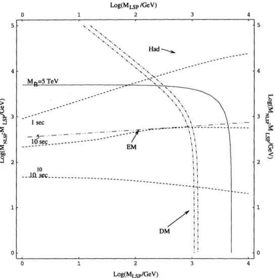
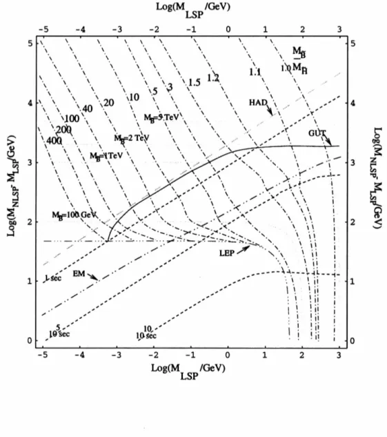
We will find that, if the Gravitino is the LSP, than all possible candidates for the NLSP are excluded by the combination of imposing gauge coupling unification and the constraint on hadronic decays coming from BBN. Just the requirement of having the Gravitino to provide all the Dark Matter of the univese and to still have gauge coupling unification would have allowed weakly interacting fermionic superpartneres as heavy as 5 TeV, with very bad consequences on the detactibility of Split Susy at LHC. This means that these constraints play a very big role. The only exception to this result occurs if the NLSP is very photino like, avoiding in this way the stringent constraints on hadronic decays coming from BBN. However, as we will see, already a small barionic decay branching ratio of 10- 3 _{is enough to rule out also this possibility.}

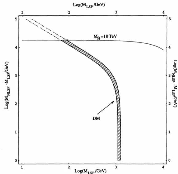
For the Extradimensional LSP, we will instead find a wide range of possibilities, with NLSP allowed to span from 30 GeV to 20 TeV.

The chapter is organized as follows. In section 4.2, we study the constraints on the spectrum coming from the requirement of obtaining gauge coupling unification. In section 4.3, we briefly review the relic abundance of Dark Matter in the case the LSP is an hidden sector particle. In section 4.4, we discuss the cosmological constraints coming from BBN and CMB. In section 4.5, we show the results for Gravitino LSP. In section 4.6, we do the same for a dark sector LSP arising in extra dimensional implementation of Split Susy. In section 4.7, we draw our conclusions.

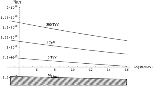
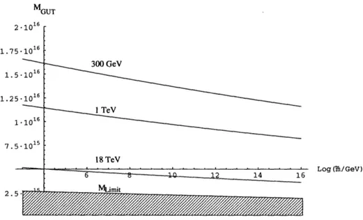
3.2 Gauge Coupling Unification

Gauge coupling unification is a necessary requirement in Split Susy theories. Here we investigate at one loop level how heavy can be the fermionic supersymmetric partner for which gauge coupling unification is allowed. We will consider the Bino, Wino, and Higgsino as degenerate at a scale M₂, while we will put the Gluinos at a different

scale M3.

Before actually beginning the computation, it is interesting to make an observation about the lower bound on the mass of the fermionic superpartners. Since the Bino is gauge singlet, it has no effect on one-loop gauge coupling unification. In Split Susy, with the scalar superpartners very heavy, the Bino is very weakly interacting, its only relevant vertex being the one with the light Higgs and the Higgsino. This means that, while for the other supersymmetric partners LEP gives a lower bound of - 50-100

GeV [11], for the Bino in Split Susy there is basically no lower limit.

Going back to the computation of gauge coupling unification, we perform the study at -loop level. The renormalization group equations for the gauge couplings are given by:

dgi 1 3

A bi(A)g (3.1)

dA (4ir)2

where bi(A) depends of the scale, keeping truck of the different particle content of the theory according to the different scales, and i = 1, 2, 3 represent respectively

/-5/3g', g, g,. We introduce two different scales for the Neutralinos, M2, and for the Gluinos M3, and for us M3 > M2.

In the effective theory below M2, we have the SM, which implies: 41 19

bM

=( -- -7)

(3.2)

9 7

bsplit2 = ( , -5) (3.4)

2' 6

and finally, above ri we have the SSM:

bssm (33

bssm 33( 1, -3) (3.5)

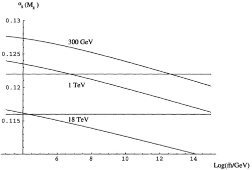
The way we proceed is as follows: we compute the unification scale MGUT and aGUT as deduced by the unification of the SU(2) and U(1) couplings. Starting from this, we deduce the value of as at the weak scale Mz, and we impose it to be within the 2 experimental result aS(Mz) = 0.119 ± 0.003. We use the experimental data:

sin2(Ow(MIz)) = 0.23150 ± 0.00016 and a- 1_{(Mz) = 128.936 ± 0.0049[12].}

A further constraint comes from Proton decay p -+ lrOe+, which has lifetime: 8fM 2M4

T(p -- roe+ ) = T((1

+

(

1016GeV aGUT \ CaN

where we have taken the chiral Lagrangian factor (1 + D + F) and the operator renormalization A to be (1 + D + F)A - 20. For the Hadronic matrix element aN, we take the lattice result [13] acN = 0.015GeV3_{. From the Super-Kamiokande limit}

[14], r(p - r°e+ ) > 5.3 x 1033yr, we get:

1/2 12GUT

MGUT> 0.01 V3) GUT/35 4 x 1015_{GeV (3.7)}

An important point regards the mass thresholds of the theory. In fact, the spec-trum of the theory will depend strongly on the initial condition for the masses at the supersymmetric scale im. As we will see, in particular, the Gluino mass M3 has a very important role for determining the allowed mass range for the Next-Lightest Supersymmetric Particle (NLSP), which is what we are trying to determine. In the light of this, we will consider M2as a free parameter, with the only constraint of being

smaller than mn. M3 will be then a function of M2 and fm, and its actual value will depend on the kind of initial conditions we require. In order to cover the larger frac-tion of parameter space as possible, we will consider two distinct and well motivated initial conditions. First, we will require gaugino mass unification at m. This initial condition is the best motivated in the approach of Split Susy, where unification plays a fundamental role. Secondarily, we will require anomaly mediated gauigino mass ini-tial conditions at the scale m. This second kind of iniini-tial conditions will give results