Isochoric, isobaric and ultrafast conductivities of aluminum, lithium and carbon in the warm dense matter (WDM) regime

Publisher’s version / Version de l'éditeur:

Condensed Matter, 2017-09-21

READ THESE TERMS AND CONDITIONS CAREFULLY BEFORE USING THIS WEBSITE. https://nrc-publications.canada.ca/eng/copyright

Vous avez des questions? Nous pouvons vous aider. Pour communiquer directement avec un auteur, consultez la

première page de la revue dans laquelle son article a été publié afin de trouver ses coordonnées. Si vous n’arrivez pas à les repérer, communiquez avec nous à PublicationsArchive-ArchivesPublications@nrc-cnrc.gc.ca.

Questions? Contact the NRC Publications Archive team at

PublicationsArchive-ArchivesPublications@nrc-cnrc.gc.ca. If you wish to email the authors directly, please see the first page of the publication for their contact information.

Archives des publications du CNRC

This publication could be one of several versions: author’s original, accepted manuscript or the publisher’s version. / La version de cette publication peut être l’une des suivantes : la version prépublication de l’auteur, la version acceptée du manuscrit ou la version de l’éditeur.

Access and use of this website and the material on it are subject to the Terms and Conditions set forth at

Isochoric, isobaric and ultrafast conductivities of aluminum, lithium

and carbon in the warm dense matter (WDM) regime

Dharma-wardana, M. W. C.; Klug, D. D.; Harbour, L.; Lewis, Laurent J.

https://publications-cnrc.canada.ca/fra/droits

L’accès à ce site Web et l’utilisation de son contenu sont assujettis aux conditions présentées dans le site

LISEZ CES CONDITIONS ATTENTIVEMENT AVANT D’UTILISER CE SITE WEB.

NRC Publications Record / Notice d'Archives des publications de CNRC:

arXiv:1710.04191v1 [physics.geo-ph] 21 Sep 2017

Isochoric, isobaric and ultrafast conductivities of

aluminum, lithium and carbon in the warm dense matter regime

National Research Council of Canada, Ottawa, Canada, K1A 0R6

L. Harbour and Laurent J. Lewis

D´epartement de Physique, Universit´e de Montr´eal, Montr´eal, Qu´ebec, Canada. (Dated: October 12, 2017)

We study the conductivities σ of (i) the equilibrium isochoric state (σis), (ii) the equilibrium isobaric state (σib), and also the (iii) non-equilibrium ultrafast matter (UFM) state (σuf) with the ion temperature Ti less than the the electron temperature Te. Aluminum, lithium and carbon are considered, being increasingly complex warm dense matter (WDM) systems, with carbon having transient covalent bonds. First-principles calculations, i.e., neutral-pseudoatom (NPA) calculations and density-functional theory (DFT) with molecular-dynamics (MD) simulations, are compared where possible with experimental data to characterize σic, σib and σuf. The NPA σib are closest to the available experimental data when compared to results from DFT+MD, where simulations of about 64-125 atoms are typically used. The published conductivities for Li are reviewed and the value at a temperature of 4.5 eV is examined using supporting X-ray Thomson scattering calculations. A physical picture of the variations of σ with temperature and density applicable to these materials is given. The insensitivity of σ to Te below 10 eV for carbon, compared to Al and Li, is clarified.

PACS numbers: 52.25.Os,52.35.Fp,52.50.Jm,78.70.Ck

I. INTRODUCTION

Short-pulsed lasers as well as shock-wave techniques can probe matter in hitherto experimentally inaccessi-ble regimes of great interest. These provide information needed for understanding normal matter and unusual states of matter, in equilibrium or in transient condi-tions [1, 2]. Similar ‘hot-carrier’ processes occur in semi-conductor nanostructures [3, 4]. Such warm dense mat-ter (WDM) systems include not only equilibrium systems where the ion temperature Ti and the electron

temper-ature Te are equal, but also systems where Ti 6= Te, or

highly non-equilibrium systems where the notion of tem-perature is inapplicable [5]. While the prediction of a quasi equation of state (quasi EOS) and related static properties for two-temperature (2T ) systems [6] is sat-isfactory, the conductivity calculations using standard codes, even for sodium at the melting point, require mas-sive quantum simulations with as much as ∼1500 atoms and over 56 k-points (according to Ref. [7]), whereas even theories of the 1980s evaluated the sodium conductivities successfully via a momentum relaxation-time (τmr)

ap-proach [8], which is also used in Drude fits to the Kubo-Greenwood (KG) formula used with density-functional theory (DFT) and molecular dynamics (MD) methods. The KG-formula and its scope are discussed further in the Appendix.

The static electrical conductivities of WDM equilib-rium systems (i.e., Ti = Te), as well as 2T

quasiequilib-rium systems, are the object of the present study. We distinguish the isobaric equilibrium conductivity σib and

the isochoric equilibrium conductivity σic from the

ul-trafast matter (UFM) quasiequilibrium (isochoric) con-ductivity σuf. The 2T WDM states exist only for times

shorter than the electron-ion equilibration time τei and

may be accessed using femtosecond probes.

We consider three systems of increasing complexity above the melting point: (a) a ‘simple’ system, viz., WDM-aluminum at density ρ =2.7 g/cm3

; (b) WDM-lithium at 0.542 g/cm3_{; and (c) WDM-carbon (2.0-3.7}

g/cm3_{) including the low-T covalent-bonding regime. As}

experimental data are available for the isobaric evolution of Al and Li starting from their nominal normal densities and down to lower densities of the expanded fluid, we cal-culate σib for Al and Li. The ultrafast conductivity σuf

is calculated for all three materials, as σisis conveniently

accessible via short-pulse laser experiments.

The electrons in WDM-Li are known to be non-local with complex interaction effects. For instance, cluster-ing effects may appear [9] as the density is increased. WDM-carbon is a complex liquid with transient cova-lent bonding where the C-C bond energy Eccmay reach

∼ 8 eV in dilute gases. The three conductivities σic,

σib, and σuf for Al, Li and C, are calculated via two

first-principles methods where, however, both finally use a ‘mean-free path’ model to estimate the conductivity. The two methods are: (i) the neutral pseudoatom (NPA) method as formulated by Perrot and Dharma-wardana [6, 10–12] together with the Ziman formula, and (ii) the DFT+MD and KG approach as available in codes such as VASP and ABINIT [13], enabling us to assess the ex-tent of the agreement among these theoretical methods and the available experiments. The liquid-metal exper-imental data are still the most accurate data on WDM systems available; they are used where possible to com-pare with calculations.

Accurate experimental data for the isobaric liquid state of Al [14, 15] and Li [17] are available, and provide a

test of the theory. No reliable isobaric carbon data are available; carbon at 3.7-3.9 g/cm3

and 100-175 GPa was studied recently by x-ray Thomson scattering (XRTS) [18]. Hence we evaluate only σicand σibin this case, for

ρ in the range of XRTS experiments and related simula-tions [19]. The conductivity across a recently-proposed phase transition [20] in low-density carbon (∼ 1.0 g/cm3

) near T ≃ 7 eV is not addressed here.

DFT+MD methods treat hot plasmas as a thermally evolved sequence of frozen solids with a periodic unit cell of N atoms — typically N ∼ 100, although order-of-magnitude larger systems may be needed [7] for reli-able transport calculations. The static conductivity σ is evaluated from the ω → 0 limit of the KG σ(ω) using a phenomenological model (e.g., the Drude σ(ω) [7, 21] or modified Drude forms [22]). More discussion of these issues is given in the Appendix. The N -ion DFT+MD model does not allow an easy estimate of single-ion prop-erties, e.g., the mean number of free electrons per ion ( ¯Z) or ion-ion pair potentials.

The NPA methods, e.g., that of Perrot and Dharma-wardana, reduce the many-electron, many-ion prob-lem to an effective one-electron, one-ion probprob-lem using DFT [10, 11, 48]. A Kohn-Sham (KS) calculation for a nucleus immersed in the plasma medium provides the bound and free KS states. While bound states remain localized within the Wigner-Seitz (WS) sphere of the ion for the regime studied here, the free electron distribution nf(r) of each ion resides in a large “correlation sphere”

(CS) such that all gij(r) → 1 as r → Rc. We typically use

Rc = 10rws, i.e., a volume of some 1000 atoms. Several

average-atom models [23, 24] have similarities and signif-icant differences among them and with the NPA method. These are reviewed in the Appendix and in Ref. [20]. The NPA method applies for low T systems even with tran-sient covalent bonding. Hence, we differ from Blenski et al. [24] who hold that “... all quantum models seem to give unrealistic description of atoms in plasma at low T and high plasma densities”. But in reality, the earli-est successful applications of the NPA were for solids at T = 0. Here we treat very low-T WDMs, e.g., Al, ρ=2.7 g/cm3

, T /EF < 0.01, using the NPA, EFbeing the Fermi

energy and obtain very good agreement for equations of state (EOS) data [6] and even for transport properties, e.g., the electrical conductivity.

The NPA static conductivity is evaluated from the Ziman formula using the NPA pseudopotential Uei(k)

and the ion structure factor S(k) [11] generated from the NPA pair potential Vii(r). The latter is used in

the hypernetted-chain (HNC) equation or its modified (MHNC) form inclusive of bridge functions, assuming spherical symmetry appropriate to fluids. HNC methods are accurate, fast and much cheaper than MD methods which fail to provide small k-information, i.e., less than ∼ 1/Lbx where Lbx is the linear dimension of the

sim-ulation box. The Ziman formula can be derived from the Kubo formula using the force-force correlation func-tion and assuming a momentum relaxafunc-tion time τmr.

0.1 1 10 100

T

(eV)

Conductivity

σ,

(10

S/m)

isobaric σ Expt., Desai-Gathers.

isobaric σ NPA Pesudop-this work.

Melting point (experimentt and NPA) isobaric DFT+MD (ABINIT)-this work isobaric-DFT+MD(VASP)-this work

isochoric σ, DFT+MD, Vlcek et al.

isochroic σ OF+MD, Sjostrom et al.

isochoric σ NPA Pseudop-this work.

isochoric σ DFT+MD -this work

ufm σ NPA-Pseudop - this work.

Al density=2.7 g/cm3 T_i = T_e T_i≠ T_e isochoric ufm isobaric (Isochoric density) Aluminum isochoric (a) (b) (c) T_i =0.06 eV v

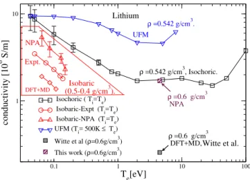
FIG. 1. (Color online) Static conductivities for Al from ex-periment and from DFT+MD and NPA calculations. The

isobaric conductivity σibis at densities 2.37 ≤ ρ ≤ 1.65 g/cm3

(cf. triangular region (a)). The isochoric (σic, region (c)) and

UFM (σuf, region (b)) conductivities are for a density of 2.7

g/cm3_{. Enlarged views of regions (a) and (c) are given in}

the Appendix. The blue-filled diamond gives the conductiv-ity of normal aluminum at its melting point (0.082 eV, 2.375

g/cm3_{), viz. σ = 4.16 × 10}6_{S/m from experiment (quoted in}

Ref. [16]) and σ = 4.09 × 106 _{S/m from the NPA.}

Zubarev’s method can also be used [25] to derive the Ziman formula. Details regarding the conductance for-mulae and their limitations are given in the Appendix.

II. THE CONDUCTIVITIES OF WDM ALUMINUM

Surprisingly low static conductivities for UFM alu-minum at 2.7 g/cm3_{, extracted from x-ray scattering data}

from the Linac Coherent Light Source (LCLS) have been reported in Sperling et al., Ref. [26]. Calculations of σic

using an orbital-free (OF) form of DFT and MD revealed sharp disagreement with the LCLS data [27]. Sperling et al.[26] found the conductivity data of Gathers [14] to dif-fers strikingly from the LCLS data and the OF results. In Fig. 4 of Ref. [26], they attempt to present a theoret-ical σic at 2.7 g/cm3that agrees approximately with the

Gathers’ data and to some extent with the LCLS data. The Gathers data are reviewed in the Appendix.

However, in our view, the LCLS, OF, and Gathers σ shouldindeed differ, in the physics involved as well as in the actual values, because:

(i) the Gathers data are for the isobaric conductivity σib

of liquid aluminum from ρ = 1.7 to 2.4 g/cm3_{(cf. region}

(a) in Fig.1).

(ii) The orbital-free simulation [27] and the DFT+MD simulations [34] are for the isochoric equilibrium (Te =

0.1 0.2 0.3 0.4 0.5

T

(eV)

Conductivity

σ,

(10

S/m)

isobaric σ Gathers’ experiment. isobaric σ NPA-this work. isobaric-DFT+MD-this work Melting Point, Experiment and NPA

ρ=1.87g/cm3 T_i = T_e Al-isobaric conductivity ρ=2.11g/cm3 ρ=1.65g/cm3 ρ=2.37g/cm3

FIG. 2. (Color online) Isobaric conductivity of aluminum from near its melting point to about 0.4 eV, expanded from Fig. 1 comparing the NPA, experiment (Gathers) and DFT+MD results. The experimental conductivity of Al at its melting point (filled blue diamond) [16], with density 2.375

g/cm3 is displayed and aligns with the NPA calculations for

the Gathers data showing the very good agreement between the NPA and two independent experiments.

(iii) The LCLS data applies to UFM-aluminum σuf, Ti6=

Te, with the ions ‘frozen’ at Ti ≃ T0, as proposed in

Ref. [40]. The UFM-conductivity is shown as region (b) in Fig. 1. The ultrafast conductivity σuf is essentially

isochoric, with Ti≃ T0at the density ρ0. The timescales

in UFM experiments are too short for (ρ, Ti) to differ

significantly from (ρ0, T0). The evaluation of the ultrafast

conductivity σuf was discussed in detail in Ref. [40], and

here we extend our study of ufm-conductivities.

A. Isobaric conductivity

In Fig.1, we globally compare our NPA-Ziman isobaric conductivities for aluminum with the isochoric and ufm conductivities, shown in regions (b) and (c). The three conductivities evolve in characteristic ways as a function of temperature.

The experimental data of Gathers for σicare compared

with our results in more detail in Fig.2, and we find ex-cellent agreementwith our NPA calculation. DFT+MD calculations using a 108-atom simulation cell are shown in both figures for σiband σic, where the PBE functional

available in VASP and ABINIT was used; they fall be-low the experimental σibor the NPA σib, a common trend

for the DFT+MD+KG σicas well, as discussed further in

the Appendix. It should be noted that Gathers gives two isobaric resistivities in columns four and five of Table-II (Ref. [14]), causing some confusion; Gathers’ results are further discussed in the Appendix.

The isochoric conductivity of Al at 0.082 eV (nominal melting point) is ≈ 5×106

S/m; the experimental isobaric conductivity [16] at the melting point is σib = 4.1 × 106

S/m, with density 2.375 g/cm3 _{instead of the}

room-temperature density of 2.7 g/cm3

due to thermal expan-sion. The value of 4.08 ×106

S/m obtained from NPA for aluminum at 2.375 g/cm3

is in excellent agreement with experiment. It is shown as a filled blue diamond symbol in figure1. This value drops to 3.8 ×106 _{S/m if}

a bridge contribution (MHNC) is not used in calculating the ion-ion structure factor.

B. Isochoric conductivity

The isochoric system, region (c) in Fig. 1, is at ρ0 =

2.7 g/cm3

, rws ≃ 2.98 a.u. (~ = |e| = me = 1), for

all T = Ti = Te. The NPA value of σic at T = 0.082

eV (nominal melting point) is ≈ 5 × 106

S/m; this is higher than the experimental value usually quoted [16] of σib= 4.1 × 106 S/m as the density of normal aluminum

becomes 2.375 g/cm3 _{instead of 2.7 g/cm}3 _{due to}

ther-mal expansion. In region (c) we see the OF conductivity of Ref. [27] going to a minimum at T ∼5 eV and subse-quently rise as T increases; DFT+MD+KG becomes in-creasingly prohibitive at these higher temperatures. The NPA calculations show a first minimum at ∼ 6 eV, fol-lowed by a maximum at 25 eV, and another minimum at ∼ 70 eV. These features in the NPA results are due to the concurrent increase in ¯Z as well as the competition between different ionization states. This effect — the conductance minimum or resistivity saturation — occurs when electrons become non-degenerate (i.e., µe≤ 0), i.e.

when all electrons (not just those near EF ∼ 12 eV) begin

to conduct.

While we favour this explanation of the minimum in the conductivity and first presented it in our discus-sion [28] of the Mlischberg experiment, some authors (e.g., R. M. More in Ref. [2], and also Faussurier et al. [29]) have proposed an explanation in terms of resistiv-ity saturation, as in Mott’s theory of minimum conduc-tance in semiconductors. The electron “mean-free path” λ = ¯vτmr, where ¯v is a mean electron velocity, is claimed

to reduce to the mean interatomic distance at resistiv-ity saturation. However, τmr evaluated using the Ziman

formula is a momentum-relaxation time associated with scattering within the thermal window of the Fermi dis-tribution at the Fermi energy (more accurately, at an energy corresponding to the chemical potential). Since 2kF is of the order of an inverse rws, it is not surprising

that one can connect a length scale related to rwsto λ.

But it does not describe the right physics of the conduc-tivity minimum. Even the simplest form of the Ziman formula already shows the conductivity minimum, and it is a single-center scattering formula using a Born ap-proximation within a continuum model; it contains no information on the interatomic distance since one can even set S(k) = 1 and obtain the resistivity saturation.

In contrast, the resistivity saturation seen in Fig. 1 for the NPA calculation manifests itself from approximately half the Fermi energy (≃ 6 eV) corresponding to ¯Z = 3, to about 70 eV corresponding to a much higher ionization of ¯Z ≈ 7. The increased ionization prevents the chemi-cal potential from becoming rapidly negative and delays the onset of the steep rise in conductivity. These features cannot be explained via a limiting mean free-path model. In fact, in an isochoric system the interionic distance does not change and one cannot have the complex structure shown in the NPA σicin such a model. For Te= 6 eV to

about T = 25 eV, ¯Z = 3 for Al and steadily converts to ¯

Z = 4, and then a decline and a rise are accompanied by the conversion of ¯Z = 4 to ¯Z ≃7 by T ∼ 70 eV.

Fig. 1 of Faussurier et al. [29] displays the isochoric re-sistivity for aluminum together with results from Perrot and Dharma-wardana [28]. However, the latter gives the scattering as well as the pseudopotential-based resistivity for aluminum where the mean electron density ¯n is held constant, not the usual isochoric resistivity where the ion density ¯ρ has to be held constant. Electron-isochoric and ion-isochoric conditions are equivalent initially and as long as ¯Z = 3 for aluminum; but the comparison be-comes misleading beyond T ≈ 15 eV. Fig. 1 of Faussurier et al.[29] also displays the aluminum isochoric resistivity from Yuan et al. [30]. However, as explained in sec. 3

of the Appendix, both Faussurier and Yuan use an ion-sphere model which leads to ambiguities in the definition of ¯Z and µ0, leading to non-DFT features which are

ab-sent in the NPA model. Hence their resistivity estimates are not directly comparable to ours. Sufficiently accu-rate experiments are not yet available at such high tem-peratures to distinguish between different theories and validate one or the other. Such models should also be tested using cases where accurate experimental data are available (e.g., in the liquid-metal regime).

A further aspect of conductivity calculations is the need to account for multiply-ionized species. For T > EF/2, ¯Z begins to increase beyond 3 and departs

sub-stantially from an integer (e.g., ¯Z = 3.5 at 20 eV ). It is thus clear that a multiple ionization model with several integral values of ¯Z, (e.g, a mixture ¯Z = 3 and ¯Z = 4) should be used, as implemented in 1995 by Perrot and Dharma-wardana [11], for lower-density aluminum. The isochoric data σic reported in Fig.1uses the

approxima-tion of a single ionic species with a mean ¯Z.

C. Ultra-fast conductivity

The nature of ultrafast matter and its properties are determined by the initial state of the system. That is, if the initial system were a room temperature solid, and if the experiment were performed with minimal delay after the pump pulse of the laser, then the ion subsystem would remain more or less intact. However, the initial state can also be the liquid state and this will lead to different results. Both these cases are studied to compare and

0.1 1 10

T_e [eV]

1

uf-condductivity [10

6 S/m]

T_i= 0.082 eV (Liquid initial state)

T_i=0.06 eV ("solid" initial state)

Aluminum. 2.7 g/cm3

FIG. 3. (Color online) Ultra-fast conductivity of Al at density

2.7 g/cm3 for (i) solid initial state at 0.06 eV, and (ii) liquid

initial state just above melting point 0.082 eV. Curve (i) was

also displayed in Fig. 1 for comparison with σiband σic.

contrast the resulting σuf for Al.

(i) For the case where the initial state is solid (FCC lattice), we assume for simplicity that the ion subsystem structure factor S(k) can be adequately approximated by its spherical average since aluminum is a cubic crystal. The major Bragg contributions are included in such an approximation. In fact, the spherically-averaged S(k) is taken to be the ion-ion S(k) of the supercooled liquid at 0.06 eV as that is the lowest temperature (closest to room temperature) where the Al-Al S(k) could be calcu-lated. The results are in fact insensitive to whether we use the S(k) at 0.06 eV, 0.082 eV (melting point) or 0.1 eV. Furthermore, here we are using the simplest local (s-wave) pseudopotential derived from the NPA approach using a radial KS equation. Hence the use of a spheri-cally average S(k) is consistent, and probably within the large error bars of current LCLS experiments (see Fig.4, Ref. [26]). The NPA σufresults (Fig.3) for the case where

the initial state is below the melting point (mimicking solid Al) have been compared in detail with the experi-mental data in Ref. [40]. Currently, no DFT+MD+KG results for σuf are available for comparison. One notes

that the σuf at Te = Ti = 0.6 eV does not go to the

conductivity of solid (crystalline) aluminum, but goes to a lower value, possibly consistent with that of a super-cooled liquid. The lower conductivity, compared to the FCC crystal is qualitatively consistent with the drop in the conductivity from the solid-state, room temperature, density = 2.7 g/cm3

value of σ ≃ 41 × 106

S/m to the liquid-state value at the melting point, 4 ×106

S/m. The drop predicted by the NPA σuf is larger. Hence this

cal-culation appears to need further improvement for T < 1.0 eV, e.g. using the structure factor of the FCC solid and including appropriate band-structure effects.

(ii) The second model we study has molten Al at its nominal melting point (0.082 eV) but at its isochoric

den-sity of 2.7 g/cm3

as the initial state. This mimics the case where the pump pulse had warmed the ion subsystem to some extent. Then we use the S(k) and pseudopoten-tials evaluated at 0.082 eV (nominal melting point), and regard that they remain unchanged while the electron screening and all properties dependent on the electron subsystem are evaluated at the electron temperature Te.

The resulting σuf is shown in Fig. 3, together with the

case where the initial state was assumed to be a temper-ature (e.g.,the room tempertemper-ature 0.026eV, or 0.06 eV) which is below the melting point. The two curves clearly suggest that the LCLS-experiments (see Ref. [40] for de-tails) for Al are more consistent with the initial state (i.e., the state of matter at the peak of the laser pulse) being solid, and with no significant pre-melt.

D. XC-functionals and the Al conductivity

Using a DFT+MD+KG approach, Witte et al. [31] ex-amined the σ for Al at ρ = 2.7 g/cm3 _{and T = 0.3 eV}

computed with the exchange-correlation (XC) function-als of (i) Perdew, Burke, and Ernzerhof (PBE) [32] and (ii) Heyd, Scuseria, and Ernzerhof (HSE) [33]. Their re-sults agree with those of Vlˇcek et al. [34] for the PBE functional; our DFT+MD calculations also agree well with those of Vlˇcek et al. as seen from the region (c) in Fig. 1. However, Witte et al. propose, from their Fig. 1, that their HSE calculation agrees [35] best with the experimental data of Gathers [14]. This is based on a calculation of the conductivity at 0.3 eV only (≈ 3500 K), which is compared with the corresponding entry in Table II, column 4, of Ref. [14], viz. resistivity=0.451µΩm, i.e., conductivity = 2.22 ×106

S/m. However, this datum is given by Gathers for a volume dilation of 1.44 (column 3), i.e., ρ = 1.875 g/cm3_{, and not 2.7 g/cm}3_{. Witte et}

al. incorrectly interprets column 4 of Gathers’ Table II as providing isochoric conductivities of Al at 2.7 g/cm3

. Gathers’ tabulation and the several resistivities given are indeed a bit confusing; we reconstruct them in Table 1 of the Appendix for convenience.

Columns 4 and 5 in Ref. [14] give two possible re-sults for the isobaric conductivity of aluminum, with col-umn 5 giving the experimental resistivity as a function of the nominal input enthalpy, i.e., “raw data”. Column 4 gives the resistivity where in effect the input enthalpy has been corrected for volume expansion; this is not the iso-choric resistivity of aluminum, as proposed by Sperling et al.[26] and by Witte et al. [31].

All the resistivities in Gathers Table II, column 4 can be recovered accurately by our parameter-free NPA cal-culation using the isobaric densities. Also, the fit formula given in the last row of table 23 of Gathers’ 1986 review [15] confirms that Table II, column 4 in Ref. [14] is indeed the final isobaric data at 0.3 GPa. Our NPA calculation at the melting recovers the known isobaric conductiv-ity [16] at 0.082 eV. which is also consistent with the Gathers data.

The HSE functional includes a contribution (e.g., 25%) of the Hartree-Fock exchange functional in it. If there is no band gap at the Fermi energy, the Hartree-Fock self-energy is such that several Fermi-liquid parameters be-come singular. Hence the use of this functional in WDM studies may lead to uncontrolled or unknown errors. Fur-thermore, previous studies, e.g., Pozzo et al. [7], Kietz-mann et al. [39], show that the PBE functional success-fully predicts conductivities. Those conductivities, if re-calculated with the HSE functional are most likely to be in serious disagreement with the experimental data.

DFT is a theory which states that the free energy is a functional of the one-body electron density, and that the free energy is minimized by just the physical den-sity. It does not claim to give, say, the one-electron ex-citation spectrum or the density of states (DOS). The spectrum and the DOS are those of a fictitious non-interacting electron system at the non-interacting density, and moving in the KS potential of the system. The KS potential is not a mean-field approximation to the many-body potential, but a potential that gives the ex-act physical one-electron density if the XC-functional is exact. Hence any claimed “agreement” between the DFT spectra and physical spectra is not relevant to the quality of the XC-functional, except in phenomenological theo-ries which aim to go beyond DFT and recover spectra, DOS, bandgaps etc., by including parameters in ‘meta-functionals’ which are fitted to a wide array of properties. There is however no theoretical basis for the existence of XC-functionals which also simultaneously render accu-rate excitation spectra, DOS and bandgaps in a direct calculation.

E. The variation of the conductivity as a function of temperature

The evolution with temperature of the conductivity can be understood within the physical picture of elec-trons near the Fermi energy (chemical potential) under-going scattering from the ions in a correlated way via the structure factor. This in turn invokes the relation of the structure factor to the Fermi momentum kF, and the

breakdown of the Fermi surface as T /EF is increased,

while the breakdown is countered by ionization which increases the Fermi energy. At sufficiently high tempera-tures the chemical potential µ tends to zero and to neg-ative values. The conductivity then becomes classical, and finally Spitzer-like. The conductivity minimum (re-sistivity plateau) in WDM systems occurs near the µ ≈ 0 region and is not related to the Mott minimum conduc-tivity.

The differences between σic and σuf, both isochoric,

arise because the structure factors S(k, Ti) of the two

systems are different, while Uei(k) and the Fermi-surface

smearing for them are essentially the same at Te, with

¯

Z ≃ 3 for Al. The ion structure factor at different temperatures, calculated using the NPA pseudopotential

0 1 2 3 4 k/k_F 0 1 2 S(k) T= 0.1 eV T= 1.0 eV T= 2.0 eV T= 5.0 eV 0 1 2 3 4 5 6 k/k_F 0 0 0.5 0.5 1 1 1.5 1.5 2 2 2.5 2.5 S(k) T=0.05 eV T=0.2 eV T=0.5 eV T=1.0 eV Al, 2.7 g/cm3 2k_F (a) (b) Li, 0.542 g/cm3 2k_F

FIG. 4. (Color online) (a) Static structure factor S(k) of

iso-choric aluminum WDM at different temperatures; S(k) at 2kF

changes by 65% from T = 0.1 to T = 5 eV. In ultrafast alu-minum S(k) remains ‘fixed’ at the initial temperature, even

when Te changes. (b) Evolution of S(k) for isochoric Li at

0.542 g/cm3 _{as a function of temperature. As T increases,}

the peak broadens and shifts away from 2kF.

Uei(k, Te) and used for evaluating σic, are shown in Fig.4

(a). The Uei and S(k), and hence σ, are first-principles

quantities determined entirely from the NPA-KS calcula-tion. If the initial temperature T0at the time of creation

of the Al-UFM were 0.082 eV (i.e., ∼melting point), then the corresponding S(k, T0) is used in evaluating σuf at all

Te, together with the Uei(k, Te). More details of σuf and

comparison with LCLS data may be found in Ref. [40]. The isobaric system differs from the isochoric and ultra-fast systems due to volume expansion. Hence the S(k) and the Uei are calculated at each ‘expanded’ density.

Degenerate electrons (Te/EF < 1) scatter from one

edge (e.g., −kF)of the Fermi surface to the opposite edge

(kF), with a momentum change k ≃ 2kF and their

scat-tering contribution essentially determines σ. Thus the position of 2kF with respect to the main peak of S(k)

and its changes with Te explain the Te dependence of

σ(Te). For aluminum at ρ = 2.7 g/cm3, 2kF lies on the

high-k side of the main peak, and as Ti = Te increases,

the peak broadens into the 2kF region (see Fig. 4(a)),

resulting in increased scattering. In the isochoric UFM case both Tiand S(k) do not change, but as Teincreases

the window of scattering f (k)(1 − f(k)) increases (here f (k) is the finite-T Fermi occupation number), and σuf

decreases.

Given that the NPA is a first-principles (i.e., ‘parameter-free’) DFT scheme, the excellent agreement between the NPA σib and the Gathers aluminum data

for σib (see Fig. 2) confirms the accuracy of NPA

pseu-dopotentials Ueiand structure factors, and enhances our

confidence in the NPA predictions for σic. In addition,

experiments at other density ranges were found to be in good agreement with NPA calculations [36] and with the DFT+MD calculations of Dejarlais et al. [37].

Further-0.1 1 10 100 T_e[eV] 1 10 conductivity [10 6 S/m] Isochoric ( T_i=T_e) Isobaric-Expt (T_i=T_e) Isobaric-NPA (T_i=T_e) UFM (T_i= 500K ≤ T_e) Witte et al (ρ=0.6g/cm3) This work (ρ=0.6g/cm3) ρ =0.6 g/cm3 NPA NPA ρ =0.6 g/cm3 DFT+MD, ρ =0.542 g/cm3. ρ =0.542 g/cm3, Isochoric. Expt. Lithium Isobaric (0.5-0.4 g/cm3). UFM DFT+MD Witte et al.

FIG. 5. (Color online) Isobaric (σib), isochoric(σic), and

ultra-fast (σuf) conductivities of Li at density 0.542 g/cm3. Isobaric

experimental conductivities σib are for 0.5 ≤ ρ ≤ 0.4 g/cm3.

The DFT+MD+KG σic value of Witte et al. at 0.6 g/cm3

and the NPA-Ziman value for σicare also shown.

more, the NPA approach becomes more reliable at higher temperatures (T /EF > 1) while the DFT+MD

meth-ods rapidly become impractical due to the large number of electronic states that are needed in the calculation due to the spread in the Fermi distribution. At lower T ion-ion correlations and interactions become important and DFT+MD treats them well. However, at low T , the higher conductivities imply longer mean free paths and the need for simulation cells with larger Lbx [38]. Good

DFT+MD+KG results, when available, provide bench-marks for calibrating other methods.

III. THE CONDUCTIVITIES OF WDM LITHIUM

The three conductivities σic, σib, and σuf for Li are

shown in Fig.5. The isobaric data are in the triangular region. The isochoric conductivities σic at a density of

ρ=0.542 g/cm3

, i.e., rws= 3.251, are given for a range of

T , while one value at ρ=0.6 g/cm3 _{and T}

e= Ti=4.5 eV,

is also given. This is for conditions reported by Witte et al. [41]. The experimental isobaric data from Oak Ridge [17] for σib (0.5 g/cm3 at 0.05 eV to 0.4 g/cm3

at 0.1378 eV), as well as the NPA σib, are also shown.

Unlike aluminum, Li is a “low electron-density” material with ¯Z = 1. Hence its EF ∼ 5 eV is small compared

to that of aluminum. For Li, 2kF lies on the low-k side

of the main peak as can be seen in Fig.4(b). The UFM conductivity σuf remains higher than the σic, and its

tem-perature dependence can be understood, as discussed in sec. II E, by the position of kF with respect to S(k) as

Te varies.

The agreement between the NPA-σib and the Oak

Ridge data for isobaric Li is moderate. The NPA-Li pseudopotential is the simplest local (s-wave) form and

0.3 0.4 0.5 0.6 0.7 0.8 density [g/cm3] 0 1 2 3 4 5 6 7 conductivity [10 6 S/m] Kietzmann DFT+MD OakRidge Expt. NPA-(this work) Kietzmann (estimated) 600K 1000K 2000K 1500K 1000K 600K 600K 1500K 1000K Lithium.

FIG. 6. (Color online) The Oak Ridge experimental data compared with the NPA and the DFT+MD+KG conductivity of Kietzmann et al. [39]. Their 600K and 1000K results have been slightly extrapolated to the low-density region covered by the experiments. The curve at 2000K given by Kietzmann

et al.is above the boiling point of Li, and is not representative

of the behaviour of Li at 1500K.

corrections (e.g., for the modified DOS) have not been used. In Fig. 6 we have attempted to compare the Oak Ridge experimental data for liquid lithium with the DFT+MD+KG calculations of Kietzmann et al. [39]. We use their calculations as a function of density for 600K and 1500K. The Kietzmann calculation at 2000K is also shown in Fig. 6, but since the boiling point of lithium under isobaric conditions is ≃ 1600K, their calculation at 2000K cannot be justifiably used to estimate a value for 1500K from the data of Kietzmann et al. which also include the two points at 600K and 1000K. Nevertheless, their results are consistent with the observed trend and agree with our NPA results to the same extent as with the Oak Ridge data.

Disconcertingly, the NPA+Ziman and the DFT+MD σic for ρ =0.6 g/cm3and T = 4.5 eV reported by Witte

et al.[41] using a 64-atom simulation cell disagree by a factor of five. But the NPA-XRTS calculations for Li (see the Appendix) agree very well with the DFT-XRTS of Witte et al.. Furthermore, we had already shown that the pair-distribution functions from NPA for Li for the density range of interest are in good agreement with the simulations of Kietzmann et al. (see Ref. [6]). However, at T =4.5 eV, µ=0.035 a.u., i.e., the plasma is nearly classical. Hence small-k scattering becomes important in determining σ. A simulation cell of length a=20.26 a.u.holds for 64 atoms. The smallest momentum accessi-ble is π/a = 0.16/(a.u.), and fails to capture the smaller-k contributions to σ. These could cause the observed dif-ferences between the NPA and DFT+MD+KG results.

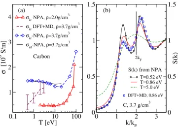
0.1 1 10 100 T [eV] 1 2 3 4 σ [10 6 S/m] σ_ic-NPA, ρ=2.0g/cm3 σ_ic DFT+MD, ρ=3.7g/cm3 σ_ic-NPA, ρ=3.7g/cm3 σuf-NPA, ρ=3.7g/cm 3 0 1 2 3 k/k_F 0 0 0.5 0.5 1 1 1.5 1.5 S(k) T=0.52 eV T=0.86 eV T=5.0 eV Carbon DFT+MD, 0.86 eV (a) (b) C, 3.7 g/cm3 2k_F S(k) from NPA

FIG. 7. (Color online) (a) Isochoric conductivity, σic, and

ultrafast conductivity σuf for carbon at ρ = 3.7 g/cm3 from

NPA and DFT+MD, and isochoric conductivity from NPA

for ρ=2.0 g/cm3_{. (b) Ion-ion S(k) for several temperatures;}

note nearly constant value of S(k) at 2kF (indicated by a

vertical line).

IV. THE CONDUCTIVITIES OF WDM CARBON

Solid carbon is covalently bonded, with strong sp3, sp2, sp bonding (with a bond energy of ∼ 8 eV) being possible. Hence efforts to create potentials extending to several neighbors, conjugation and torsional effects etc., have generated complex semi-empirical “bond-order” po-tentials parametrized to fit data bases but without any T dependence. Transient C-C bonds occur in liquid-WDM carbon. Normal-density liquid C near its melting point is a good Fermi liquid with four ‘free’ electrons ( ¯Z =4) per carbon. An early comparison of Car-Parrinello cal-culations for carbon with NPA was reported by Dharma-wardana and Perrot in 1990 [42]. NPA successfully pre-dicts the S(k) and g(r), inclusive of pre-peaks due to C-C bonding [20] as also obtained from DFT+MD sim-ulations of WDM-carbon[18, 19]. The NPA and Path Integral Monte Carlo g(r) [43] also agree closely [20]. No experimental σib are available; hence we calculate only

σic and σuf to display the remarkable difference in the

conductivities of complex WDMs with (transient) cova-lent bonding, compared to simpler WDMs like Al and Li. Figure 7(a) displays σic and σuf for isochoric carbon

at 3.7 g/cm3

. Here EF is ∼ 30 eV (for ¯Z = 4) and the

WDM behaves as a simple metal, with σ dropping as T increases, and then increasing at higher Te when µe

becomes negative. The conductivity (for T ≤ 0.5EF) is

determined mainly by the value of S(k) at 2kF, shown

in Fig.7(b). This is set by the C-C peak in S(k), which is relatively insensitive to T , and hence σ is also insensi-tive to temperature (compared to WDM Al or Li) in this regime. The insensitivity of S(k = 2kF)to temperature

ul-trafast conductivity for liquid carbon as compared to σuf

and σic of WDM-Al or Li. In WDM-carbon the

ultra-fast and isochoric conductivities are very close in magni-tude. The DFT+MD σicvalues for 3.7 g/cm3differ from

the NPA at low-T where strong-covalent bonds dominate. The N ∼ 100 atom DFT+MD simulations may be seri-ously inadequate due to such C-C bond formation. The NPA itself deals only in a spherically averaged way with the covalent bonding. That approximation is probably sufficient for static conductivities if the bonding is truly transient. In any case, accurate experimental σib data

for liquid carbon are badly needed.

V. CONCLUSION

Although it is not necessary in principle to distin-guish between isochoric and isobaric conductivities, as the specification of the density and temperature is suffi-cient, the use of such a distinction is useful in comparing experiment and theory. We see from our calculations that the temperature variations of the three conductiv-ities have distinct features. Furthermore, the ultrafast conductivity is indeed a physically distinct property as the ion subsystem remains unchanged while only the elec-tron subsystem is changed during the short time delay be-tween the pump pulse and the probe pulse. Thus in this study we have found it useful to distinguish isochoric, isobaric and ultrafast conductivities of WDM systems, using Al, Li and C as examples. The NPA σib are in

ex-cellent agreement with the aluminum experimental data of Gathers [14], while the DFT+MD+KG with 108-atom simulations estimate a lower conductivity. The NPA re-sults are in moderate agreement with Oak Ridge σib for

Li, as is also the case with DFT+MD+KG calculations. The carbon σic, σuf from NPA have a striking behaviour

in the regime of (normal) densities studied here, and dif-fer from Al and Li. We attribute this to the effect of transient C-C bonds.

Appendix

This appendix addresses the following topics:

• Neutral pseudoatom (NPA) calculation of the X-ray Thomson scattering (XRTS) ion feature W (q) for comparison with the density-functional-theory/molecular-dynamics (DFT+MD) calcula-tions of Witte et al. [41], where the excellent agree-ment is in clear contrast to the disagreeagree-ment for the conductivity datum for Li reported by Witte ıet al.

• Details of the neutral pseudoatom (NPA) model.

• Ziman formula for the conductivity using the NPA pseudopotential and the ion-ion structure factor S(k).

• Examples of DFT+MD and KG calculations for Al, Li, and C, and Drude fits to the KG conductivity of Al and Li.

• Review of the isobaric and the isochoric conductiv-ities of aluminum in the context of the experiment of Gathers, and the disagreement with the conduc-tivity of Al reported in Fig.1 of Ref. [31] by Witte et al. using the Heyd, Scuseria, and Ernzerhof (HSE) functional. 0 1 2 3 4 5 6 7 8 k [Å-1] 0 1 2 3 4 q(k), f(k), N(k), W(k)

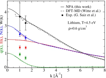
NPA (this work) DFT-MD (Witte et al.) Exp. (G. Saiz et al.)

Lithium, T=4.5 eV ρ=0.6 g/cm3

FIG. 8. (Color on line) Comparison of quantities

rele-vant to XRTS calculated using NPA+HNC (this work) and DFT+MD (Witte et al. [41]) for lithium. Values for k smaller

than about 0.6/˚A are not available from the DFT+MD

simu-lation due to the finite size of the simusimu-lation cell. Here q(k) is the Fourier transform of the free-electron density at the Li ion in the plasma, while f (k) is the bound-electron form factor

and N (k) = f (k) + q(k). The ion feature W (k) = N (k)2_S(k)

involves the ion-ion structure factor S(k). Experimental

points are from Saiz et al. (2008) cited in Witte et al., Fig. 8

1. X-ray Thomson Scattering calculation for Li at density ρ = 0.6 g/cm3 _{and temperature T = 4.5 eV.}

The calculation of XRTS of WDM using the NPA method has been described in detail in Ref. [46]. The XRTS ion feature W (k) for Li at T = 4.5 eV and ρ = 0.6 g/cm3 _{has been calculated (see Fig.8) to compare our}

NPA results with the results from the DFT+MD simula-tions by Witte et al. (Ref. [41], Fig.8). This establishes the excellent agreement with the electronic structure part of the NPA calculation and the ionic part, Sii(k),

re-sulting from the DFT+MD calculations, irrespective of the exchange-correlation (XC) functional used. That is, while we have used the local-density approximation (LDA) of the finite-T XC functional Fxc based on the

classical-map hyper-netted-chain scheme (CHNC) [44], Witte et al. have used the T = 0

Perdew-Burke-Ernzerhof (PBE) XC functional [32] which includes gra-dient corrections.

The mean ionization ¯Z for Li obtained in the NPA is unity, in agreement with that used by Witte et al.. They calculate the quantities q(k), f (k), N (k), and W (k) = N (k)2_{S(k). The quantity q(k) is the ‘screening cloud’,}

i.e., the Fourier transform of the free-electron density at the Li ion in the plasma, while f (k) is the bound-electron form factor. Their sum is denoted by N (k) = f (k)+q(k). Finally, W (k) = N (k)2_{S(k) is the ion feature and}

in-volves the ion-ion structure factor S(k).

The excellent accord between our XRTS calculation and that of Witte et al. establishes that our S(k), electron charge distributions, and potentials Uei(k) and

Vii(k) are fully consistent with the structure data and

electronic properties coming from DFT+MD. The S(k) and Uei(k) are the only inputs to the Ziman formula for

σ0. Nevertheless, our estimate of the conductivity

dis-agrees strongly with the Kubo-Greenwood estimate of Witte et al. . Given the relatively good agreement that we found with the Oak Ridge experimental data, as well as with the Kietzmann data (see Fig. 6), this disagree-ment is a priori quite surprising; one possible contrib-utory factor will be taken up in our discussion of the Kubo-Greenwood formula, viz., that it may be caused by the use of a small 64-atom DFT+MD simulation cell. The conductivity estimate by Witte et al. for T=0.3 eV at 2.7 g/cm3

is also problematic and it is taken up below, in our discussion of Gathers’ results for aluminum.

2. Details of the NPA model and ¯Z

The NPA model used here [11, 12] has been described in many articles; we summarize it again here for the convenience of the reader, as it should not be assumed that it is equivalent to various currently-available ion-sphere (IS) average-atom (AA) models such as Purgato-rio [45] used in many laboratories. While these models are closely related, they invoke additional considerations which are outside DFT. We regard the NPA model as a rigorous DFT model based on the variational prop-erty of the grand potential Ω([n], [ρ]) as a functional of both one-body densities n(r) and ρ(r), directly leading to two coupled KS equations where the unknown quanti-ties are the XC-functional for the electrons and the ion-correlation functional for the ions [47]. Approximations arise in modeling those XC-functionals and decoupling the two KS equations for simplified numerical work.

The NPA model assumes spherical symmetry when dealing with fluid phases, and calculates the KS states of a nucleus of charge Z immersed in an electron gas of input density ¯n. The ion distribution ρ(r) is approx-imated by a neutralizing uniform positive background containing a cavity of radius rws, with the nucleus at

the origin. The Wigner-Seitz (WS) radius rws is that of

the ion-density ¯ρ, i.e., rws = {3/(4π ¯ρ)}1/3. The effect

of the cavity is subtracted from the final result where

by the density response of a uniform electron gas to the nucleus is obtained. The validity of this approach has been established in previous work, for the WDM systems investigated here and reviewed in Ref. [10]. The solution of the KS equation extends up to Rc = 10rws, defining

a correlation sphere (CS) large enough for all electronic and ionic correlations with the central nucleus to have gone to zero. The WS cavity plays the role of a nominal ρ(r) to create a pseudoatom which is a neutral scatterer and greatly facilitates the calculation. The KS equations produce two groups of energy states, viz, negative and positive with respect to the energy zero at r → ∞ out-side the CS. States in one group decay exponentially to zero as r → Rc, and in fact become negligible already

for r → rws in the case of low-Z elements. These states,

fully contained within the WS sphere, are deemed bound states, and allow one to define a mean ionization per ion, Zb = Z − nb, where nb is the total number of electrons

in the bound states and Z is the nuclear charge: Zb= Z − nb; nb = X nl 2(2l + 1) Z d~rfnl|φnl(r)|2. (A.1) Here fnl = 1/{1 + exp(xnl)}, xnl = {ǫnl − µ0}/T is

the Fermi factor for the KS state φnl with energy ǫnl.

The non-interacting electron chemical potential µ0 is

used here. Furthermore, there are plane-wave-like phase-shifted KS states which extend through the whole corre-lation sphere. These are continuum states and their elec-tron population is the free-elecelec-tron distribution nf(r).

The nucleus Z, the bound electrons nb, the cavity with

a charge Zc = (4π¯n/3)r3ws and the free electrons form

a neutral object and hence it is a weak scatterer called the ‘neutral pseudoatom’ (NPA). The Friedel sum ZF

of the phase shifts of the continuum states and the cav-ity charge Zc add up to zero when the KS-equations are

solved self-consistently. Thus Zc= ZF = 2 πT Z ∞ 0 kfklk{1 − fkl} X l (2l + 1)δl(k)dk. (A.2) Here fkl is the Fermi occupation factor for the k, l-state

with energy ǫ = k2

/2. Full self-consistency requires that Zb= Zc= ZF, ¯n = ¯Z ¯ρ. (A.3)

Hence, given an input mean free-electron density ¯n, the WS radius (equivalently ¯ρ) is iteratively adjusted till self-consistency is obtained, i.e., Eq. A.3 is satisfied to a chosen precision. The mean ionization ¯ρ is thus seen to be the Lagrange multiplier ensuring charge neutral-ity, as first discussed in Ref. [48]. The ¯ρ resulting from the input ¯n may not be the required physical ion density, and hence several values of ¯n and the corresponding ¯ρ are determined to obtain the actual ¯n that corresponds to the required experimental ion density ¯ρ. This process produces a unique value of ¯Z, and the problem of having several different estimates of ¯Z, as found in IS-AA mod-els [23, 45] does not arise here. The agreement among

ZF, Zc, Zb is essential to the convergence of the

NPA-KS equations. It is sensitive to the exchange-correlation (XC)-functional Fxc(T ) and to the proper handling of

self-interaction (SI) corrections, whenever ¯Z is close to a half-integer. Using a valid ¯Z is essential to obtaining good conductivities.

We emphasize that a key difference between IS models and the NPA is that the free electrons are not confined to the Wigner-Seitz sphere, but move in all of space as ap-proximated by the correlation sphere. These differences are discussed in Sec. 3.

In this study we use the local-density approximation to the finite-T XC-functional as parametrized by Perrot and Dharma-wardana [44]. This simplest implementation (in LDA) is a useful reference step needed before more elab-orate implementations (involving SI, non-locality, etc. in the XC-functionals) are used.

Since ¯Z is the free-electron density per ion, it can de-velop discontinuities whenever the ionization state of the element under study changes due to, e.g., increase of T or compression. This behaviour is analogous to the for-mation or disappearance of band gaps in solids. In fact, if the NPA model is treated with periodic boundary con-ditions, as for a solid with one atom in the unit cell, then the discontinuity in Z appears as the problem of correctly treating the formation of a gap in the density of states (DOS) at the Fermi energy. A proper evaluation of such features in the DOS and band gaps is difficult in DFT as this is a theory of the total energy as a functional of the one-body density, not a theory of individual energy levels. The one-electron states are given by the Dyson equation. Thus band-structure calculations inclusive of GW-corrections are used in solids to obtain realistic band gaps and excitation energies. In dealing with discontinu-ities in ¯Z, a similar procedure is needed [49], including the use of self-interaction (SI) corrections and XC func-tionals that include electron-ion correlation corrections, i.e., Fei(n, ρ) [47, 50].

It should be mentioned that some authors have claimed that ¯Z “does not correspond to any well-defined observ-able in the sense of quantum mechanics” [51],i.e, that there is no quantum operator corresponding to ¯Z. This view is incorrect as quantities like the temperature T , the chemical potential µ, and the mean ionization ¯Z are quantities in quantum statistical physics. There may be no operator for them in simple T = 0 quantum theo-ries. In most formulations of quantum statistical physics these appear as Lagrange multipliers related to the con-servation of the energy, particle number and charge neu-trality. They can also be incorporated as operators in more advanced field-theoretic formulations of statistical physics (e.g., as in “thermofield-dynamics” of Umezawa). Some of these broader issues are discussed in Chapter 8 of Ref. [52].

Finally, it is noted that the mean number of elec-trons per ion, viz., ¯Z in, e.g., gas-discharge plasmas, is routinely measured using Langmuir probes, or derived from optical measurements of various properties

includ-ing the conductivity and the XRTS profile [53] for WDM-plasmas. Hence ¯Z is a well-established measurable prop-erty.

3. Some Differences between the NPA model and typical average-atom models

To our knowledge, no conductivity calculations using the Purgatorio model for isobaric aluminum are available for comparison with experimental data. Such a compari-son is also problematic due to the lack of an unequivocal value for the mean ionization ¯Z in IS-AA models [45]. We list several differences with the NPA which particularly affect conductivity calculations:

1. Most average-atom models are based on the IS-AA model where the free-electron pileup around the nucleus is strictly confined to the Wigner-Seitz sphere:

¯ Z = 4π

Z Rws 0

∆nf(r)r2dr; IS-AA model. (A.4)

This condition, Eq.A.4, was used in Salpeter’s early IS model, in the Inferno model of Lieberman, and in codes like Purgatorio [45] derived from it, to determine an elec-tron chemical potential µ0

ws. It is also used in Yuan et

al.[30], Faussurier et al. [29], Starrett and Saumon [54], and in other AA codes discussed in Murillo et al. [23]. However, µ0

ws is not identical with the non-interacting

µ0 because it includes a confining potential applied to

the free electron density nf(r) constraining the electrons

to the IS. As it is applied via a boundary condition, it is a non-local potential. The KS XC potential is also a non-local potential and hence the use of Eq.A.4 con-taminates the XC potential. On the other hand, DFT is based on mapping the interacting electrons to a system of non-interacting electrons whose chemical potentially is rigorously µ0, as used in the NPA model that we employ.

In the NPA we use a CS with a large radius Rc.

¯ Z = π

Z Rc 0

∆nf(r)r2dr; NPA model. (A.5)

The upper limit of the integral is Rc≈ 10rwsand hence

deals with a sphere large enough for all correlations with the central ion to have died down at the surface of the sphere. This enables the use of the non-interacting chem-ical potential in the NPA, as needed in DFT, since all equations use the large-r limit beyond the CS as the ref-erence state.

The constraint placed by Eq.A.4is clearly invalid at low temperatures where the de Broglie wavelength of the electrons, being proportional to 1/√T , exceeds rws at

sufficiently low T . Hence such AA-models become invalid at low temperatures and are not true DFT models. In contrast, the first successful applications of the NPA (in the 1970s) were to low-temperature solids.

2. The use of the constraint placed by Eq.A.4in AA models has far reaching consequences as it prevents the

possibility of providing a unique definition of the mean ionization, as emphasized by Stern et al. [45] in regard to the Inferno code. In fact even at high temperatures, there are at least two definitions of ¯Z that differ, and hence the estimates of the electrical conductivity are not unambigu-ous. This is not the case in the NPA. The problem of discontinuities in ¯Z and the under-estimate of bandgaps by DFT theory were already discussed in the previous subsection.

3. The IS-AA models do not satisfy a Friedel sum rule for ¯Z, while the f -sumrule is also constrained by the condition imposed by Eq.A.4.

4. As the electrons are confined to the WS sphere in IS-AA models, they cannot display pre-peaks due to transient covalent bonding as found in liquid carbon, hy-drogen and other low-Z WDMs. This was confirmed by Starrett et al. [55] for carbon for their AA model. The bonding occurs by an enhanced electron density in the inter-ionic region between two WS spheres, and this is not allowed in IS models. In contrast, the NPA model shows pre-peaks in gii(r) corresponding to transient C-C

bonding in liquid carbon, and produces a pair-potential with a minimum corresponding to the C-C covalent bond distance at sufficiently low T [20]. Similar pre-peaks are found via NPA calculations for warm-dense hydrogen and low-Z elements in the appropriate temperature and den-sity regimes [62].

4. Pseudopotentials and pair-potentials from the NPA

The KS calculation for the electron states for the NPA in a fluid involves solving a simple radial equation. The continuum states φk,l(r), ǫk = k2/2, with occupation

numbers fkl, are evaluated to a sufficiently large energy

cutoff and for an appropriate number of l-states (typi-cally 9 to 39 were found sufficient for the calculations presented here). The very high-k contributions are in-cluded by a Thomas-Fermi correction. This leads to an evaluation of the free-electron density nf(r), and the

free-electron density pileup ∆n′

(r) = nf(r)−¯n. A part of this

pileup is due to the presence of the cavity potential. This contribution m(r) is evaluated using its linear response to the electron gas of density ¯n using the interacting elec-tron response χ(q, Te). The cavity corrected free-electron

pileup ∆nf(r) = ∆n′(r) − m(r) is used in constructing

the electron-ion pseudopotential as well as the ion-ion pair potential Vii(r) according to the following equations

(in Hartree atomic units) given for Fourier-transformed

quantities: Uei(k) = ∆nf(k)/χ(k, Te), (A.6) χ(k, Te) = χ0(k, Te) 1 − Vk(1 − Gk)χ0(k, Te) , (A.7) Gk = (1 − κ0/κ)(k/kTF); Vk= 4π/k2,(A.8) kTF= {4/(παrs)}1/2; α = (4/9π)1/3, (A.9) Vii(k) = Z2Vk+ |Uei(k)|2χee(k, Te). (A.10)

Here χ0 is the finite-T Lindhard function, Vk is the bare

Coulomb potential, and Gk is a local-field correction

(LFC). The finite-T compressibility sum rule for electrons is satisfied since κ0 and κ are the non-interacting and

in-teracting electron compressibilities respectively, with κ matched to the Fxc(T ) used in the KS calculation. In

Eq.A.9, kTFappearing in the LFC is the Thomas-Fermi

wavevector. We use a Gk evaluated at k → 0 for all k

in-stead of the more general k-dependent form (e.g., Eq. 50 in Ref. [44]) since the k-dispersion in Gkhas negligible

ef-fect for the WDMs of this study. Steps towards a theory using self-interactions corrections in the Fxc, a modified

electron DOS, self-energy corrections etc., have also been given [49]. In this study we use the above equations, and only in the LDA.

5. Calculation of the ion-ion Structure factor

The ion-ion structure factor S(k) is also a first-principles quantity as it is calculated using the ion-ion pair potential, Eq.A.10 given above. For simple fluids like aluminum we use the modified hyper-netted-chain (MHNC) equation. g(r) = exp{−βVii(r) + h(r) − c(r) + B(r)},(A.11) h(r) = c(r) + ¯ρ Z d~r1h(~r − ~r1)c(~r1), (A.12) h(r) = g(r) − 1. (A.13)

Here c(r) is the direct correlation function. Thermody-namic consistency (e.g., the virial pressure being equal to the thermodynamic pressure) is obtained by using the Lado-Foiles-Ashcroft (LFA) criterion (based on the Gibbs-Bogoliubov bound for the free energy) for deter-mining B(r) using the hard-sphere model bridge func-tion [56]. That is, the hard-sphere packing fracfunc-tion η is selected according to an energy minimization that sat-isfies the LFA criterion. The iterative solution of the MHNC equation, i.e., Eq. (A.11), and the Ornstein-Zernike (OZ) equation, Eq. (A.12), yield a gii(r) for the

ion subsystem. The LFA criterion and the associated hard-sphere approximation can be avoided if desired, by using MD with the pair potential to generate the g(r). The hard-sphere packing fraction η calculated via the LFA criterion is the only parameter extraneous to the KS scheme used in our theory. In calculating the S(k) of complex fluids like carbon, where the leading peak in g(r) is not determined by packing effects but by transient C-C bonding, we use the simple HNC equation.

0 0.1 0.2 ω [a.u.] 0 0.5 1 1.5 2 2.5 3 Conductivity σ(ω) [10 6 S/m] KG-σ(ω) Drude fit 0 0.1 0.2 ω [a.u.] 0 0.5 1 1.5 0 0.4 0.8 ω [a.u.] 0 0.4 0.8 KG-σ(ω) 1eV KG-σ(ω) 0.5 eV Aluminum T = 1 eV. (a) ρ=2.7 g/cm3 Lithium T = 0.108 eV. ρ=0.432g/cm3 (b) ρ=3.7g/cm3 (c) Carbon

FIG. 9. (Color online) KG conductivity σ(ω) for Al, Li, and C. Note the slight non-Drude behaviour of Li σ(ω) near 0.08 a.u. in panel (b). The carbon σ(ω) is highly non Drude-like, with the peak moving to higher energy as T is lowered; no Drude form is shown for carbon.

6. Calculation of the electrical conductivity

The electrical conductivity is calculated from the nu-merically convenient form of the Ziman formula given in Ref. [11]. The Ziman formula is sometimes derived from the Boltzmann equation. However, the KG for-mula and also the Ziman forfor-mula can both be derived from the Fermi golden rule [57]. The Ziman formula uses the ‘momentum-relaxation time’ approximation, while the KG formula typically uses the same approximation when extracting the static conductivity using a Drude fit to the dynamic conductivity σ(ω). The Ziman formula used here is:

σ = 1/R R = (~/e2 )(3π¯n ¯Z)−1 I (A.14) I = Z ∞ 0 q3_Σ(q)dq 1 + exp{β(ǫq/4 − µ)} , (A.15) ǫq = (~q2/2m), β = 1/T, (A.16)

Σ(a) = S(q)|Uei(q)/{2πε(q)}|2, (A.17)

1/ε(q) = 1 + Vqχ(q, T ). (A.18)

The “Born-approximation-like” form used here is valid to the same extent that the pseudopotential Uei(q)

con-structed from the (non-linear) KS nf(r) via linear

re-sponse theory (Eq. A.7) is valid. The S(k) used are available even for small-k unlike in DFT+MD simula-tions where the smallest accessible k-value is limited by the finite size Lbx of the simulation cell.

7. The Kubo-Greenwood conductivity

The KG dynamic conductivity σ(ω) is a popular ap-proach to determining the static conductivity of WDM systems via DFT+MD [59]. In our simulations we have

used N =108 atoms in the simulation cell, with a 2 ×2×2 Monkhorst-pack k grid; the PBE XC functional was used. The energy cutoff was taken to be sufficiently high that the occupations in the highest KS states were virtually negligible. The quenched-crystal KS-eigenstates φν(r)

and eigenvalues ǫν, where ν is a band-index quantum

number, are used in the Kubo-Greenwood conductivity as provided in the standard ABINIT code. Usually six to ten such evaluations were obtained by evolving the quenched crystal by further MD simulations (using only the Γ point), and in each case the σ(ω) was obtained – see Fig.9 for typical aluminum, lithium and carbon results for σ(ω).

The aluminum σ(ω) is well-fitted by the Drude form: σ(ω) = σ0/(1 + (ωτ )

2

), σ0= ¯nτ. (A.19)

However, there is no justification for using a Drude form for carbon. The peak position in σ(ω) roughly corre-sponds to the ‘bonding → antibonding’ transition in the fluid containing significant covalent bonding (see Fig. 4(b) of the main text) at 0.5 eV. This is seen from the strong peak in g(r) near 3 a.u. (1.55 ˚A ) corresponding to the C-C bond length. This suggests that the N = 108 simulation is quite inadequate for complex liquids like carbon, as bonding reduces the effective N of the simu-lation. In the case of carbon, the static limit of the KG σ(ω) was simply estimated from the trend in the ω → 0 region rather than using a Drude fit. Furthermore, the different quenched crystals (108 atoms in the simulation) gave significant statistical variations, as reflected in the error bars shown in Fig. 4(a) of the main text. At higher T , e.g., for T = 1 − 2 eV, the estimated conductivity behaves similar to that from the NPA, but somewhat less conductive. The KG formula does not include any self-energy corrections in the one-electron states and ex-citation energies, and less importantly, no ion-dynamical contributions either, as the ions are stationary (Born-Oppenheimer approximation). The form of σ(ω) includ-ing ion dynamics has been discussed by Dharma-wardana at the Carg`ese NATO work shop in 1992 [58].

8. The conductivity of Li at T =4.5 eV and density 0.6 g/cm3

The conductivity of Li, at density ρ = 0.6 g/cm3

at 4.5 eV estimated by Witte et al. [41], is roughly a factor of five less than that obtained from NPA+Ziman. While the NPA calculation may differ from another calculation by, at worst, a factor of 2, it is hard to find an explanation for this strong disaccord, given the good agreement in the XRTS calculation. One possibility is the use of a 64-atom cell in DFT+MD for Li at a chemical potential µ ∼ 0. DFT+MD and KG using N ∼ 100 atoms in the simulation seems to significantly underestimate σ0

for low-valence substances like Li, Na, especially as T is increased. Low-valence materials have a small µ = EF

0.1 0.2 0.3 0.4 0.5 0.6

T

(eV)

Conductivity

σ,

(10

S/m)

isochroic σ OF+MD, Sjostrom et al.

isochoric σ NPA Pseudop-this work.

isochoric σ DFT+MD (VASP)-this work

Witte et al, PBE functional

isochoric σ Vlcek et al. DFT+MD

Witte et al, HSE functional

T_i = T_e

Al, 2.7 g/cm3

Isochoric Al, 2.7 g/cm3

FIG. 10. (Color online) Isochoric conductivity of aluminum from near its melting point to about 0.7 eV, expanded from Fig. 1 of the main text, and now including the Witte et al. [31] calculation of the Al-conductivity at 0.3 eV and ρ = 2.7

g/cm3_{. Our DFT+MD data and those of Vlˇcek are shown.}

values where small-k scattering is important, and finally to µ < 0 values (classical regime).

At low T /EF the major contributions to σ are provided

by electron scattering between −kFand kF, kF =√2EF,

i.e., momentum changes of the order of 2kF. However,

at finite T , µ replaces EF, and as T increases µ → 0

and to negative values. The scattering momenta near µ → +0 are in the small-k region, These contribute sig-nificantly to σ at T = 4.5 eV for Li at 0.6 g/cm3_{. In Li,}

if a 64-atom simulation is used, an appropriate length a of the cubic simulation cell would be a = 20.26 a.u. The smallest momentum accessible by such a simulation is π/a=0.16/(a.u.) and hence the corresponding Kubo-Greenwood formula will not sample the small k < 0.16 region. We see from Fig.8also that the DFT+MD simu-lations do not provide values for k smaller than ≈ 0.6/˚A due to the finite size of the cell used in Ref. [31].

Hence such DFT+MD+KG calculations of σ are strongly weighted to the larger-k strong scattering regime and predict a low conductivity. The results of Pozzo et al., where a 1000-atom simulation was needed for Na is a case in point. However, such large simulations are be-yond the scope of many laboratories while NPA-type ap-proaches usually provide results to within a factor of two in the worst case.

9. Isobaric and isochoric conductivity of aluminum in the liquid-metal region

High-quality experimental data (errors of ± 6 %) are available for the isobaric conductivity σib of liquid

alu-minum at low T [14, 15]. The relevant region, viz.,

(a) of Fig. 1 of the main text, is shown enlarged to display the experimental and calculated data in Fig. 2. The NPA calculation is in excellent agreement with the experiment of Gathers, to well within the error bars. On the other hand, the DFT+MD calculation captures about 75% of the experimental conductivity. A ∼100-atom simulation cannot capture the k-values smaller than π/a ∼ 0.12/(a.u.) for Al at this density, and may con-tribute to some of the under-estimate.

Isochoric conductivities (with ρ = 2.7 g/cm3_{) of}

alu-minum obtained from the NPA and from DFT+MD by us and by Vlˇcek et al. [34] are shown in Fig.10, together with a single data point from Witte et al. [31] with the PBE functional, and with the HSE functional. The re-sult obtained using the HSE XC-functional is a strong underestimate compared to other DFT+MD [60, 61], the orbital-free calculation and the NPA estimates.

In Ref. [31] Witte et al. strongly argue for the HSE functional even for aluminum, a ‘simple’ metal proven to work well with more standard approaches. The value of 2.23 ×106 _{S/m quoted by them at 0.3 eV, 2.7 g/cm}3_{, is}

taken to agree with experiment, based on their interpre-tation of the experimental data of Gathers [14]. However, as discussed below, Gathers’ datum at 0.3 eV (≃3500K) is for isobaric aluminum at ρ = 1.875 g/cm3

and 0.3 GPa.

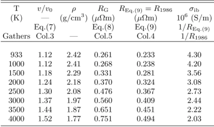
10. The experimental data of Gathers

Gathers measures the resistivity of aluminum in an isobaric experiment, starting from the solid (ρ0=2.7

g/cm3_{, v}

0=0.37 cm3/g) and heating to the range 933K to

4000K at 0.3 GPa [14]. Gathers himself recommends the Gol’tsova-Wilson [63, 64] volume expansion data rather than those measured by him. In Table II of the 1983 publication of Gathers [14], the experimental resistivity (“raw data”) calculated using the nominal enthalpy in-put to the sample is given in column 5. The apparatus and the sample undergo volume expansion; the resistivi-ties for the input enthalpy corresponding to the volume expanded sample (using the Gol’tsova-Wilson data) are given in column 4 of the same table. Hence the “volume corrected” isobaric resistivity for aluminum in the range (T =993K, ρ=2.42g/cm3

) to (T =4000K, ρ=1.77g/cm3

) are the values found in column 4 while column 5 gives the “raw data”. Column 4 resistivities agree with the isobaric resistivity values that may also be obtained from the fit formula given in the last row of Table 23 of the 1986 Gathers review[15].

Since Table II as given by Gathers is somewhat mis-leading, we have recalculated the resistivities R using the fit equations given by Gathers. Eq. (8) gives the (expansion-uncorrected) “raw data”, labeled RG. The

expansion correction essentially brings the input heat to the actual volume of the sample. Thus equation (9), where the enthalpy input is corrected for volume expan-sion agrees with Gathers’ fit equation given subsequently in 1986 [15] and hence labeled R1986. Gathers uses the