Testing the Attraction Effect on Two Information Visualization Datasets

HAL Id: hal-01295624

https://hal.inria.fr/hal-01295624

Submitted on 29 Nov 2016

HAL is a multi-disciplinary open access

archive for the deposit and dissemination of

sci-entific research documents, whether they are

pub-lished or not. The documents may come from

teaching and research institutions in France or

abroad, or from public or private research centers.

L’archive ouverte pluridisciplinaire HAL, est

destinée au dépôt et à la diffusion de documents

scientifiques de niveau recherche, publiés ou non,

émanant des établissements d’enseignement et de

recherche français ou étrangers, des laboratoires

publics ou privés.

Distributed under a Creative Commons Attribution - ShareAlike| 4.0 International

License

Testing the Attraction Effect on Two Information

Visualization Datasets

Evanthia Dimara, Anastasia Bezerianos, Pierre Dragicevic

To cite this version:

Evanthia Dimara, Anastasia Bezerianos, Pierre Dragicevic. Testing the Attraction Effect on Two

Information Visualization Datasets. [Research Report] RR-8895, Inria Saclay Ile de France. 2016,

pp.13. �hal-01295624�

ISSN 0249-6399 ISRN INRIA/RR--8895--FR+ENG

RESEARCH

REPORT

N° 8895

Project-Team AVIZ and ILDA

Testing the Attraction

Effect on Two

Information Visualization

Datasets

RESEARCH CENTRE SACLAY – ÎLE-DE-FRANCE

Parc Orsay Université 4 rue Jacques Monod 91893 Orsay Cedex

Testing the Attraction Effect on Two Information

Visualization Datasets

Evanthia Dimara

, Anastasia Bezerianos

, Pierre Dragicevic

Project-Team AVIZ and ILDA

Research Report n° 8895 — March 2016 — 14 pages

Abstract: The attraction effect is a well-studied cognitive bias in decision making research, where people’s choice between two options is influenced by the presence of an irrelevant (dominated) third option. In another article, we report on two crowdsourced experiments showing compelling evidence that the attraction effect can generalize to visualizations. However, we also conducted another experiment between the two where we failed to observe an effect. This experiment used scatterplots generated from real datasets, and restricted participants’ choice between exactly two alternatives. In accordance with the principle of full reporting, we report on this experiment and discuss the possible reasons for this negative result.

Key-words: Negative result, information visualization, decision-making, decoy effect, attraction effect, asymmetric dominance effect, cognitive bias

∗_{Evanthia Dimara is with Inria, Université Paris-Saclay and Université Paris-Sud; email: evanthia.dimara@inria.fr}

†_{Anastasia Bezerianos is with Université Paris-Sud, CNRS & Inria, Université Paris-Saclay; email: anastasia.bezerianos@lri.fr} ‡_{Pierre Dragicevic is with Inria; email: pierre.dragicevic@inria.fr}

Test de l’effet d’attraction sur deux jeux de données

de visualisation d’information

Résumé : L’effet d’attraction est un biais cognitif souvent étudié dans la recherche en prise de décision, et selon lequel un choix entre deux options est influencé par la présence d’une troisième option non pertinente (dominée). Dans un autre article, nous décrivons deux expériences qui montrent que l’effet d’attraction se généralise aux visualisations. Cependant, nous avons aussi conduit une autre expérience où nous n’avons pas pu observer d’effet. Cette expérience a employé des nuages de points générés à partir de jeux de données réelles, et a restreint les choix à exactement deux options. Nous décrivons ici cette expérience et discutons les raisons possibles de ce résultat négatif.

Mots-clés : Résultat négatif, visualisation d’information, prise de décision, effet d’attraction, effet de leurre, effet de domination asymétrique, biais cognitif

Testing the Attraction Effect on Two Information Visualization Datasets 3

Education

Crime control

Bob Alice Eve

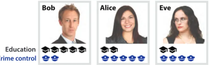
Figure 1: Example of an attraction effect in elections: Bob has an excellent education plan, while Alice is very strong in crime control. The addition of Eve, a candidate similar but slightly inferior to Alice, raises Alice’s attractiveness as a candidate. This irrelevant option is called a decoy. (Photos Benjamin Miller, FSP Standard License, icons by Ivan Boyco, CC-BY license)

1

Introduction

The attraction effect (also called decoy effect or asymmetric dominance effect) is a well-studied cognitive bias in the psychology of decision making and in consumer behavior research, where people’s choice between two options is influenced by the presence of an irrelevant (dominated) third option (Huber et al, 1982; Huber and Puto, 1983; Ariely and Wallsten, 1995). Figure 1 shows an example.

The attraction effect has been so far only tested with small option sets (i.e., two alternatives plus a decoy) and simple presentation formats such numerical tables, text and pictures, but not visualizations. Since visualizations can be used to support decision-making — e.g., when choosing a house (Williamson and Shneiderman, 1992), a nursing home (Yi, 2008), a financial investment (Daradkeh et al, 2013), or a software feature to support (Aseniero et al, 2015) — such an effect could have important implications.

In a separate article (Dimara et al, 2016), we report on two crowdsourced experiments showing good evidence that the attraction effect can generalize to visualizations. However, we conducted another exper-iment between the two experexper-iments reported, where we failed to observe an effect despite a large sample size (n = 297). This experiment differs in two major respects from the other two: i) it uses real datasets known in the infovis domain (the “car dataset” and the “house dataset”), and ii) it uses a constrained choicetask, where only two of all alternatives are available. In accordance with the principle of full reporting (Cumming, 2013) and in order to prevent publication bias (Anderson, 2012; The Economist, 2013), we report on this experiment here, and discuss the possible reasons for this negative result.

More extensive information on the attraction effect, the related literature, the motivations for this work, and the rationale for the methods employed can be found in the main article (Dimara et al, 2016).

2

Design Rationale

In the first experiment “Gyms” reported in (Dimara et al, 2016), we found evidence for an attraction effect in scatterplots by replicating a standard experimental protocol. However, the datasets are limited to 2 or 3 alternatives, which is not realistic for a dataset people may want to visualize. The main reason for this limitation of previous work is that in numerical table representations it is hard to perform rapid attribute-to-attribute comparisons, and thus recognition of dominance relationships, between many alternatives.

Scatterplots and other visualizations are designed to remove these barriers, and facilitate rapid spatial comparisons of many data points. Thus, we hypothesized that in scatterplots with many alternatives, a sufficient number of decoys will also increase the attractiveness of the target. We decided to test this in a second experiment, using sets of alternatives derived from two real datasets. In this research report we describe the motivation, design rationale and results of this experiment, referred to as experiment “Real”. A later, third experiment involving artificially generated scatterplots and referred to as experiment “Bets”, is reported in Dimara et al (2016), with positive results.

4 Dimara & Bezerianos & Dragicevic

2.1

Additional Terminology

This section extends the terminology introduced in Dimara et al (2016)-Sections 2.2.1 and 4.2.

The Pareto front is the set of all alternatives that are not dominated in a decision task (Ottosson et al, 2009). In other words, it is the set of all possible choices that are not obviously “wrong”. All alternatives in a Pareto front are formally uncomparable. In a classical attraction effect experiment (Figure 1), the Pareto front consists of only two alternatives: the target and the competitor.

Let T1be a decision task where only two choices A and B are available on the Pareto front. Let T2be

another decision task that only differs from T1in that it contains additional alternatives, all dominated by

Abut not by B. We will refer to these additional alternatives as decoys on A, to the alternative A as the target, and to the alternative B as the competitor. These definitions are consistent with the definitions from Dimara et al (2016)-Section 4.2. Concrete examples of such cases will be provided later on.

A constrained choice task is a decision task that requires choosing an option from a subset of all the alternatives. We will refer to this subset as the choice set. A classical attraction effect experiment is not a constrained choice task, since the choice set is the same as the set of alternatives.

2.2

Stimuli and Task

As in Dimara et al (2016)-Experiment Gyms, we chose a 2D scatterplot to visually represent the sets of alternatives, one of the common infovis representations of large bi-dimensional datasets. This time we did not include a numerical table as a control condition, since numerical tables do not support rapid com-parisons among many alternatives. Instead we looked at how the addition of decoys shifts participants’ choice between target and competitor.

In numerical tables or other textual formats, people need to actively perform pairwise comparisons to see dominance relations between alternatives. According to Crosetto and Gaudeul (2014), the decision task in an attraction effect experiment can be broken in two stages: i) a dominance recognition stage, where participants exclude the dominated alternative; and ii) a final selection stage, where participants choose one of the two non-dominated alternatives based on their preference.

Our concern regarding the extension of attraction effect in scatterplots was that the dominance recog-nition task – i.e. the exclusion of multiple decoys– could be time consuming or error-prone for crowd-source participants, given the large number of alternatives. Since we were interested in the selection stage of the task, we decided to eliminate the dominance recognition part of the task by restricting participants’ choice set to two non-dominated alternatives. We focused on only two alternatives instead of the full Pareto front to remain consistent with the target/competitor dichotomy used in studies on the attraction effect and to avoid interaction with other cognitive biases, as explained in Dimara et al (2016).

Thus, we used a constrained choice task whose the choice set consisted in two formally uncomparable alternatives picked on the Pareto front. As we can see in the stimuli shown in Figures 4, 5, 6, and 7, we indicated target and competitor in red color –whereas other data points were in gray– and we labeled them as A and B. Participants indicated their choice of A and B in a radio button below the diagram.

2.3

Scenario and Attribute Values

Previous research has studied how different positions of a single decoy influence the effect, and it is believed that positions are not all of the same weight. For instance, Huber et al (1982) found the attraction effect increasing in the dimension on which the target is the weakest (i.e., the dimension where the competitor is superior). Despite the differences in attraction intensity depending on position, the effect seems to persist regardless of where we place a single decoy (Wedell, 1991). However, the decoys so far have been studied in one position at a time (single decoy), rather than having multiple decoys, at different positions at the same time, as is our case.

Testing the Attraction Effect on Two Information Visualization Datasets 5 2.3.1 Dataset Selection

Since we are interested in the attraction effect with many alternatives shown on scatterplots, for this second experiment we based our tasks on real datasets. We started with a corpus of five multidimensional tabular datasets containing information on houses, cars, cameras, cereals and movies1_{. These datasets}

are routinely used in the infovis community for the purposes of teaching, designing and demonstrating multidimensional data visualization systems (e.g., Elmqvist et al (2008); Yi et al (2005)).

For each dataset we examined all possible 2D scatterplots and searched for distributions that were roughly linear (such as in Figure 2), indicating a trade-off between the two attributes. In addition, each attribute should be easy to understand, and as we discussed in (Dimara et al, 2016), should exhibit a clear direction of preference. For example, carbohydrate content from the cereals dataset is not a good choice of attribute, since some people might seek low carbohydrate content while others might seek the opposite, and some may not even understand what it means. Only two datasets (cars and houses) had attributes pairs that had a roughly linear relationship and where each attribute was easy to understand and had clear direction of preference. We chose a pair of attributes for each of these datasets. More specifically, the two bi-dimensional datasets we extracted from our corpus were:

• The cars dataset, a set of 407 car models from America, Japan and Europe manufactured from 1970 to 1982, described according to their horsepower and their fuel efficiency in miles per gallon. • The houses dataset, a set of 781 real estate listings in the San Luis Obispo area from 2009, described

according to their size in square feet and their price in US dollars.

Although the car and real estate markets have significantly evolved since the data was collected, the trade-offs involved remain the same and thus decision making tasks should not be impacted.

2.3.2 Dataset Preparation

We cleaned up the chosen datasets by i) removing all duplicate alternatives — i.e., houses or cars with identical attribute values, and ii) removing alternatives more than two standard deviations away from the mean on either of their two attributes. This prevented outliers from excessively compressing the scales of the scatterplot axes. A total of 61 duplicates and 37 outliers were removed from the car dataset, and 16 duplicates and 43 outliers were removed from the house dataset.

We then removed outliers along the Pareto front on each of the two datasets. This was done by per-forming a linear regression on the Pareto front and removing all alternatives whose standardized residual was greater than two. Doing so eliminated alternatives that may appear attractive only because they present an unusually good trade-off. One such outlier was removed from the car dataset, and two from the house dataset. Figure 2 shows the two datasets, their Pareto front, and the discarded outliers.

1_{More information on these datasets is provided at http://www.aviz.fr/decoy}

Horsepower MPG Size Pr ice Cars Houses

Figure 2: The cars and houses datasets with their Pareto front, in blue. Crosses are discarded outliers.

6 Dimara & Bezerianos & Dragicevic A B A B A B A B RA RB RAB R0 RP RA RB RAB R0 RP RA RB RAB R0 RP RA RB RAB R0 RP

-

--

-

-D

D

D

D

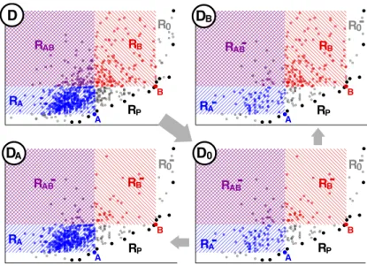
Figure 3: The house dataset D and three possible subsets (D0, DAand DB) created by randomly removing

alternatives in specific regions.

We then chose two alternatives A and B on the Pareto front to act as target and competitor. The alternatives A and B were chosen so as to maximize |RA| + |RB| as defined below.

We then generated three subsets from each dataset as follows2. Let D be the full set of alternatives (cars or houses), P its Pareto front, {A, B} the choice set, dAall alternatives dominated by A, and dBall

alternatives dominated by B (see blue and red hatchings respectively in Figure 3 D). We partitioned Din five regions: RA= dA\ dB; RB= dB\ dA; RAB= dA∩ dB; RP= P; and R0= D \ (dA∪ dB∪ P).

We then randomly eliminated 80% of the alternatives from the sets RA, RB and RAB, and 50% of the

alternatives in R0, yielding the subsets R−A, R − B, R

− AB, and R

−

0. From this we constructed three sets of

alternatives, shown in Figure 3: D0= R−A∪ R − B∪ R − AB∪ R − 0 ∪ RP; DA= RA∪ R−B∪ R − AB∪ R − 0 ∪ RP and DB= R−A∪ RB∪ R−AB∪ R − 0 ∪ RP.

It can be seen in Figure 3 that the only difference between D0 and DA is that DA contains more

alternatives that are dominated by A but not by B. These asymmetrically dominated alternatives are analogous to decoys, while A plays the role of a target and B plays the role of a competitor. Note however that no artificial choice is added: all points belong to the original dataset, including the decoys. The roles of A and B are swapped when comparing D0to DB. The final stimuli can be seen in Figures 4 to 7.

2.4

Measures

As with the Bets experiment in Dimara et al (2016), we measure the attraction effect by the difference in the proportion of participants who chose the target in the condition with decoys vs. the condition without decoys. If p(X )S is the proportion of participants who chose X in the set of alternatives S,

our data subsets allow for two possible measures of the attraction effect: EA= p(A)DA− p(A)D0 and

EB= p(B)DB− p(B)D0. A third aggregated measure EAB= EA+ EBreferred to as the combined attraction

effectis possible that combines the two effects and has been used in past studies (Wedell, 1991). Since EAB= p(A)DA− p(A)DB, the combined measure can be calculated without knowing the responses for D0.

To maximize statistical power, we therefore chose to only present the decision tasks DAand DB, and use

EABas the measure of attraction effect. We report this measure for both the cars and the houses dataset. 2_{The construction described here is slightly different than that of (Dimara et al, 2016), but the resulting regions are equivalent.}

Testing the Attraction Effect on Two Information Visualization Datasets 7

Figure 4: Cars dataset, decoys on A Figure 5: Cars dataset, decoys on B

Figure 6: Houses dataset, decoy on A Figure 7: Houses dataset, decoy on B

2.5

Crowdsource Quality Control

Similar to the Gyms experiment (Dimara et al, 2016), we defined rejection criteria in advance and cate-gorized jobs as Red (rejected) and Green (kept for analysis). There was no Orange category this time.

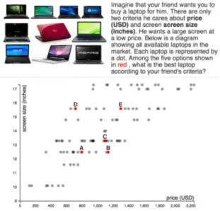
Similar to the Gyms experiment, we made sure that participants were able to read a scatterplot. How-ever, since our new scatterplots have many more data points, our screening test was more advanced: participants had to pick the dominant option among five options shown in red, among other unavailable options shown in gray (Figure 8). Furthermore, we measured attention with a simple catch question, by asking participants at the end of the job to recall whether the study was about houses and cars, or about other topics (e.g., cameras and cars).

A job was classified as Red if the contributor failed the scatterplot test, took an abnormal amount of time to complete the job (<1 min or >30 min), or failed the final catch question. Out of the 302 crowdsource jobs submitted with a valid completion code, 71 (24%) were categorized as Red, and 231 (76%) were classified as Green and kept for analysis.

3

Experiment Design

The experiment followed a mixed design. The independent between-subjects variable was the decoy position(on A or on B), while the independent within-subjects variable was the dataset (houses or cars). Each participant was presented with two decision tasks, one for each dataset. We varied the decoy position within each dataset, resulting in 2×2 = 4 different pairs of decision tasks. In addition, we counterbalanced the order of appearance of the two datasets, resulting in 8 unique sequences of tasks3.

3_houses

A-carsA, housesA-carsB, housesB-carsA, housesB-carsB, carsA-housesA, carsA-housesB, carsB-housesA, carsB-housesB.

8 Dimara & Bezerianos & Dragicevic

Figure 8: The scatterplot reading test. The answer was provided through a radio button.

As explained in subsection 2.4 our dependent variable was the combined attraction effect, i.e., the difference between the proportion of participants who chose option A when it was the target, and the pro-portion of participants who chose option A when the target was B. We compute and report the attraction effect for the houses dataset and for the cars dataset separately.

3.1

Participants

Our study was completed by 231 crowdflower contributors of high quality (level 3) based on their per-formance on the platform, and whose job was classified Green. Their demographics as reported in a post-test questionnaire is summarized in Figure 9 (middle map and stacked bar charts labeled “Real”), together with the demographics of the previous experiment “Gyms” and the next experiment “Bets” (Di-mara et al, 2016). As we can see, the demographics between the three experiments are very similar.

Bets Real Gyms

Gender Education

No schooling completed, or less than 1 year Nursery, kindergarten, and elementary (grades 1-8) Some high school, no diploma High school (grades 9-12, no degree) High school graduate (or equivalent) Some college (1-4 years, no degree) Associate’s degree (occupational & academic) Bachelor’s degree (BA, BS, AB, etc) Master’s degree (MA, MS, MENG, MSW, etc) Professional school degree (MD, DDC, JD, etc) Doctorate degree (PhD, EdD, etc)

F M 15-24 25-34 35-44 45-54 55-79 Age Bets Real Gyms Bets 73 participants Real 231 participants Gyms 305 participants

Figure 9: Self-reported location, gender, age and education of the participants for all three experiments: the experiment “Real” reported here, and the experiments “Gyms” and “Bets” in Dimara et al (2016).

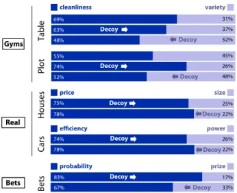
Testing the Attraction Effect on Two Information Visualization Datasets 9 cleanliness variety 31% 37% 52% 45% 26% 48% 69% 63% 48% 55% 74% 52% power price size 75% 78% 74% 78% 25% 22% 26% 22% probability prize Table Plot 83% 67% 17% 33% Houses Bets Cars Bets Real Gyms Decoy Decoy Decoy Decoy Decoy Decoy Decoy Decoy Decoy Decoy

Figure 10: Proportions of participant choices in all three experiments, the experiment “Real” reported here, and “Gyms” and “Bets” reported in Dimara et al (2016).

3.2

Procedure

Pre-test: As explained before and shown on Figure 8, participants were first tested on their basic ability to read a scatterplot. Participants who failed this test were removed from the analysis.

Task: Participants then opened a 9-page online form which took on average 5 minutes to complete. For the house dataset, they were asked to imagine that they want to buy a house, and that all houses were similar apart from two attributes: size and price. They were then shown a scatterplot with 792 dots representing the houses in the market. Participants were told that they narrowed down their choices to two houses, shown in red. As seen before, the two red dots were labelled A and B, and all other dots where shown in gray. Participants indicated their choice using a separate radio button below the scatterplot. On the next page, they rated their confidence in their choice, justified their choice in a text area, and reported the level of their familiarity with the real estate market. After that (or before, depending on the task ordering), they had to carry out a similar task with a scatterplot displaying 356 cars according to power and efficiency. Participants could review previous pages on the form but not change their answers. Post-task questions: Participants then had to fill a short questionnaire with their demographic informa-tion, and were given the attention test mentioned previously.

3.3

Hypothesis

Our statistical hypothesis was that the combined attraction effect will be positive for both datasets.

4

Results

Experimental stimuli, data and analysis scripts are available at http://www.aviz.fr/decoy.

4.1

Planned Analyses

All analyses reported here were planned before data was collected. Participant choices are shown in Figure 10, bars labeled “Real”. The top two bars are the proportion of responses for the house dataset,

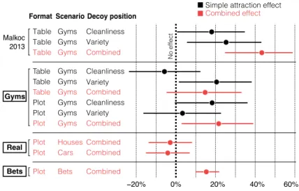
10 Dimara & Bezerianos & Dragicevic Table Table Table Table Table Table Plot Plot Plot Plot Plot Plot Gyms Gyms Gyms Gyms Gyms Gyms Gyms Houses Cars Bets Cleanliness Variety Variety Combined Combined Cleanliness Cleanliness Variety Combined Combined Combined Combined Gyms Gyms −20% 0% 20% 40% 60% Simple attraction effect Combined effect Malkoc 2013 Gyms Decoy position Scenario Format Real Bets No effect

Figure 11: Point estimates and 95% confidence intervals for the attraction effects in Malkoc et al. Malkoc et al (2013), and in all our three experiments: the experiment “Real” reported here, and “Gyms” and “Bets” reported in Dimara et al (2016).

with decoys on price (A) at the top, and on size (B) at the bottom. The next two bars are the responses for the cars dataset, with decoys on efficiency (A) on the top, and power (B) on the bottom. The decoys are expected to increase the proportion of choices of the target, in the direction indicated by the arrows. As can be seen, this was not the case for either dataset, and the combined attraction effect was even negative in both cases, although small (-3% and -4%).

We now turn to inferential statistics, reported in Figure 11 for all our experiments. The two combined attraction effects mentioned previously are shown in red next to the label “Real”. The two dots indicate the point estimates reported previously, and error bars are 95% confidence intervals that indicate the uncertainty around those estimates (Cumming and Finch, 2005). Confidence intervals were computed using score intervals for difference of proportions and independent samples. The combined attraction effect was -3%, CI [-14%, +8%] for houses, and -4% , CI [-15%, +7%] for cars.

Thus, the apparent reversal of the attraction effect observed in Figure 10 is way too unreliable for any conclusion to be drawn concerning the direction of the effect (Cumming and Finch, 2005). We can only be reasonably confident that the effect is no larger than 15% in either direction. If there is indeed an attraction effect, it is clearly smaller than the combined effect obtained by Malkoc et al (2013) using the classical procedure, and likely smaller than the effect we previously obtained in our Gyms experiment. A “repulsion” effect is also possible. In summary, our results in this experiment are largely inconclusive.

4.2

Additional Analyses

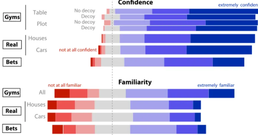
As can be seen in Figure 12, participants reported similar levels of confidence in their answers across both datasets. For the houses dataset, participants reported a mean level of confidence of 6.0 on a 7-point Likert scale. For cars the mean confidence was 5.9. When it comes to familiarity, responses were diverse for both houses and cars as can be seen in Figure 12, but on average, people were similarly familiar with both datasets (both means 4.2).

Testing the Attraction Effect on Two Information Visualization Datasets 11 Houses Cars Plot Table Gyms Real Bets Houses Cars All Familiarity

not at all familiar extremely familiar

Gyms Real Bets Decoy Decoy No decoy No decoy

Figure 12: Self-reported familiarity and confidence in all three experiments: experiment “Real” reported here, and experiments “Gyms” and “Bets” reported in Dimara et al (2016).

5

General Discussion and Conclusion

One major reason for these inconclusive results is a lack of statistical power: since the effect seems small, we would need a remarkably large sample size (i.e., much larger than N=231) or a modified design to be able to reliably assess both the direction and the magnitude of the effect.

Our inability to detect an effect at least indicates that in this experiment, the manipulation we used was not sufficient to trigger the same attraction effect as the effects typically observed in more typical experiments. Attempting to interpret this finding a-posteriori, it may be due to the choice of a constrained decision task. As explained in the background section in (Dimara et al, 2016), the attraction effect requires that participants recognize the dominance relationship between the target and the decoy. Although our participants could read scatterplots (we used a screening test) and the scatterplots we used gave them the opportunity to perceive and to recognize these dominance relationships, it is possible that the dominated alternatives (and thus the decoys) were ignored. Since these alternatives were not part of the choice set, it may have been more clear to participants that they were not needed to carry out the task. In classical attraction effect experiments it is also the case that the decoy is irrelevant to the decision task, but participants have to determine its irrelevance (i.e., perform dominance recognition) themselves. The visual design of the scatterplot (i.e., the two available options shown in red, all other options in gray) may have reinforced the impression that non-available alternatives could be entirely ignored. The disregard of decoys could have also been reinforced by the way participants gave their answers (radio buttons, one for each of the two red choices).

Given this possible interpretation as well as the low statistical power of the experiment considering the effect size investigated, it is premature to conclude that the attraction effect does not exist in scatterplots. This is particularly the case as we were able to replicate a classical attraction effect (one target, one competitor, one decoy) using scatterplots in our experiment “Gyms” (Dimara et al, 2016). We thus decided to conduct a third experiment, reported in Dimara et al (2016) as experiment “Bets”, where we modified the choice procedure (any alternative can be selected), the datasets (synthetically generated to maximize the effect), and the experiment design (within-subjects to maximize statistical power). We were able to find compelling evidence for an attraction effect, but more realistic datasets like the ones described here remain to be tested.

12 Dimara & Bezerianos & Dragicevic

References

Anderson G (2012) No result is worthless: the value of negative results in science. Online, URL http: //tinyurl.com/anderson-negative, last accessed Mar 2015

Ariely D, Wallsten TS (1995) Seeking subjective dominance in multidimensional space: An ex-planation of the asymmetric dominance effect. Organizational Behavior and Human Decision Processes 63(3):223 – 232, DOI http://dx.doi.org/10.1006/obhd.1995.1075, URL http://www. sciencedirect.com/science/article/pii/S0749597885710758

Aseniero BA, Wun T, Ledo D, Ruhe G, Tang A, Carpendale S (2015) Stratos: Using visualization to support decisions in strategic software release planning. In: Proceedings of the 33rd Annual ACM Conference on Human Factors in Computing Systems, ACM, pp 1479–1488

Crosetto P, Gaudeul A (2014) Testing the strength and robustness of the attraction effect in con-sumer decision making. Jena Economic Research Papers 2014-021, Friedrich-Schiller-University Jena, Max-Planck-Institute of Economics, URL http://EconPapers.repec.org/RePEc:jrp: jrpwrp:2014-021

Cumming G (2013) The new statistics: why and how. Psychological science

Cumming G, Finch S (2005) Inference by eye: confidence intervals and how to read pictures of data. American Psychologist 60(2):170

Daradkeh M, Churcher C, McKinnon A (2013) Supporting informed decision-making under uncertainty and risk through interactive visualisation. In: Proceedings of the Fourteenth Australasian User Interface Conference-Volume 139, Australian Computer Society, Inc., pp 23–32

Dimara E, Bezerianos A, Dragicevic P (2016) The attraction effect in information visualization. Under review.

Elmqvist N, Dragicevic P, Fekete JD (2008) Rolling the Dice: Multidimensional Visual Explo-ration using Scatterplot Matrix Navigation. IEEE Transactions on Visualization and Computer Graphics 14(6):1141–1148, DOI 10.1109/TVCG.2008.153, URL https://hal.inria.fr/ hal-00699065, best Paper Award

Huber J, Puto C (1983) Market boundaries and product choice: Illustrating attraction and substitution effects. Journal of Consumer Research pp 31–44

Huber J, Payne JW, Puto C (1982) Adding asymmetrically dominated alternatives: Violations of reg-ularity and the similarity hypothesis. Journal of Consumer Research 9(1):90–98, URL http:// EconPapers.repec.org/RePEc:ucp:jconrs:v:9:y:1982:i:1:p:90-98

Malkoc SA, Hedgcock W, Hoeffler S (2013) Between a rock and a hard place: The failure of the attraction effect among unattractive alternatives. Journal of Consumer Psychology 23(3):317 – 329, DOI http: //dx.doi.org/10.1016/j.jcps.2012.10.008, URL http://www.sciencedirect.com/science/ article/pii/S1057740812001295

Ottosson RO, Engström PE, Sjöström D, Behrens CF, Karlsson A, Knöös T, Ceberg C (2009) The fea-sibility of using pareto fronts for comparison of treatment planning systems and delivery techniques. Acta Oncologica 48(2):233–237

The Economist (2013) Unreliable research: Trouble at the lab. Online, URL http://tinyurl.com/ trouble-lab, last accessed Mar 2015

Testing the Attraction Effect on Two Information Visualization Datasets 13 Wedell DH (1991) Distinguishing among models of contextually induced preference reversals. Journal of

Experimental Psychology: Learning, Memory, and Cognition 17(4):767

Williamson C, Shneiderman B (1992) The dynamic homefinder: Evaluating dynamic queries in a real-estate information exploration system. In: Proceedings of the 15th Annual International ACM SIGIR Conference on Research and Development in Information Retrieval, ACM, New York, NY, USA, SI-GIR ’92, pp 338–346, DOI 10.1145/133160.133216, URL http://doi.acm.org/10.1145/ 133160.133216

Yi JS (2008) Visualized decision making: development and application of information visualization tech-niques to improve decision quality of nursing home choice

Yi JS, Melton R, Stasko J, Jacko JA (2005) Dust & magnet: multivariate information visualization using a magnet metaphor. Information Visualization 4(4):239–256

14 Dimara & Bezerianos & Dragicevic

Contents

1 Introduction 3

2 Design Rationale 3

2.1 Additional Terminology . . . 4

2.2 Stimuli and Task . . . 4

2.3 Scenario and Attribute Values . . . 4

2.3.1 Dataset Selection . . . 5

2.3.2 Dataset Preparation . . . 5

2.4 Measures . . . 6

2.5 Crowdsource Quality Control . . . 7

3 Experiment Design 7 3.1 Participants . . . 8 3.2 Procedure . . . 9 3.3 Hypothesis . . . 9 4 Results 9 4.1 Planned Analyses . . . 9 4.2 Additional Analyses . . . 10 5 General Discussion and Conclusion 11

RESEARCH CENTRE SACLAY – ÎLE-DE-FRANCE

Parc Orsay Université 4 rue Jacques Monod 91893 Orsay Cedex

Publisher Inria

Domaine de Voluceau - Rocquencourt BP 105 - 78153 Le Chesnay Cedex inria.fr